| Issue |
A&A
Volume 511, February 2010
|
|
|---|---|---|
| Article Number | A21 | |
| Number of page(s) | 10 | |
| Section | Planets and planetary systems | |
| DOI | https://doi.org/10.1051/0004-6361/200912700 | |
| Published online | 25 February 2010 | |
The HARPS search for southern extra-solar planets
XIX. Characterization and dynamics of the
GJ 876 planetary system![[*]](/icons/foot_motif.png) ,
,
A. C. M. Correia1,2 - J. Couetdic2 - J. Laskar2 - X. Bonfils3 - M. Mayor4 - J.-L. Bertaux5 - F. Bouchy6 - X. Delfosse3 - T. Forveille3 - C. Lovis4 - F. Pepe4 - C. Perrier3 - D. Queloz4 - S. Udry4
1 - Departamento de Física, Universidade de Aveiro, Campus de Santiago,
3810-193 Aveiro, Portugal
2 - IMCCE, CNRS-UMR8028, Observatoire de Paris, UPMC, 77 avenue
Denfert-Rochereau, 75014 Paris, France
3 - Laboratoire d'Astrophysique, Observatoire de Grenoble, Université
J. Fourier, CNRS-UMR5571, BP 53, 38041 Grenoble, France
4 - Observatoire de Genève, Université de Genève, 51 ch. des
Maillettes, 1290 Sauverny, Switzerland
5 - Service d'Aéronomie du CNRS/IPSL, Université de Versailles
Saint-Quentin, BP 3, 91371 Verrières-le-Buisson, France
6 - Institut d'Astrophysique de Paris, CNRS, Université Pierre et Marie
Curie, 98 bis Bd Arago, 75014 Paris, France
Received 15 June 2009 / Accepted 6 October 2009
Abstract
Precise radial-velocity measurements for data acquired with the HARPS
spectrograph infer that three planets orbit the
M 4 dwarf star GJ 876. In particular, we
confirm the existence of planet d, which
orbits every 1.93785 days. We find that its orbit may have
significant eccentricity (e = 0.14), and deduce a
more accurate estimate of its minimum mass of ![]() .
Dynamical modeling of the HARPS measurements combined with literature
velocities from the Keck Observatory strongly constrain the orbital
inclinations of the b and c
planets. We find that
.
Dynamical modeling of the HARPS measurements combined with literature
velocities from the Keck Observatory strongly constrain the orbital
inclinations of the b and c
planets. We find that ![]() and
and ![]() ,
which infers the true planet masses of
,
which infers the true planet masses of ![]() and
and ![]() ,
respectively. Radial velocities alone, in this favorable case, can
therefore fully determine the orbital architecture of a multi-planet
system, without the input from astrometry or transits. The orbits of
the two giant planets are nearly coplanar, and their 2:1 mean motion
resonance ensures stability over at least 5 Gyr. The libration
amplitude is smaller than
,
respectively. Radial velocities alone, in this favorable case, can
therefore fully determine the orbital architecture of a multi-planet
system, without the input from astrometry or transits. The orbits of
the two giant planets are nearly coplanar, and their 2:1 mean motion
resonance ensures stability over at least 5 Gyr. The libration
amplitude is smaller than ![]() ,
suggesting that it was damped by some dissipative process during planet
formation. The system has space for a stable fourth planet in a 4:1
mean motion resonance with planet b, with a period
around 15 days. The radial velocity measurements constrain the
mass of this possible additional planet to be at most that of the
Earth.
,
suggesting that it was damped by some dissipative process during planet
formation. The system has space for a stable fourth planet in a 4:1
mean motion resonance with planet b, with a period
around 15 days. The radial velocity measurements constrain the
mass of this possible additional planet to be at most that of the
Earth.
Key words: stars: individual: GJ 876 - planetary systems - techniques: radial velocities - methods: observational - methods: numerical - celestial mechanics
1 Introduction
Also known as IL Aqr, GJ 876 is only 4.72 pc away from our Sun and is thus the closest star known to harbor a multi-planet system. It has been tracked by several instruments and telescopes from the very beginning of the planetary hunt in 1994, namely the Hamilton (Lick), HIRES (Keck) echelle spectrometers, ELODIE (Haute-Provence), and CORALIE (La Silla) spectrographs. More recently, it was also included in the HARPS program.
The HARPS search for southern extra-solar planets
is an extensive radial-velocity survey of some 2000 stars in
the solar neighborhood conducted with the HARPS spectrograph on the
ESO 3.6-m telescope at La Silla (Chile) in the
framework of Guaranteed Time Observations granted to the HARPS building
consortium (Mayor
et al. 2003).
About 10% of the HARPS GTO time were dedicated to observe a
volume-limited sample of ![]() 110 M dwarfs.
This program has proven to be
very efficient in finding Neptunes
(Bonfils
et al. 2007,2005b) and Super-Earths
(Forveille
et al. 2009; Mayor et al. 2009;
Udry
et al. 2007) down to
110 M dwarfs.
This program has proven to be
very efficient in finding Neptunes
(Bonfils
et al. 2007,2005b) and Super-Earths
(Forveille
et al. 2009; Mayor et al. 2009;
Udry
et al. 2007) down to ![]() .
Because M dwarfs are more
favorable targets to searches for lower mass and/or cooler planets than
around
Sun-like stars, the observational effort dedicated by ESO has
increased by a factor of four, to an extended sample of
300 stars.
.
Because M dwarfs are more
favorable targets to searches for lower mass and/or cooler planets than
around
Sun-like stars, the observational effort dedicated by ESO has
increased by a factor of four, to an extended sample of
300 stars.
The first planet around GJ 876, a Jupiter-mass planet
with a period of about 61 days, was simultaneous reported by Delfosse et al. (1998)
and Marcy et al.
(1998). Later, Marcy
et al. (2001) found that the 61-day signal was
produced by two planets in a 2:1 mean motion resonance, the inner one
with 30-day period also being a gas giant.
While investigating the dynamical interactions between those two
planets,
Rivera et al. (2005)
found evidence of a third planet, with an orbital period less than
2 days and a minimum mass of 5.9 ![]() ,
which at that
time was the lowest mass detected companion to a main-sequence star
other than
the Sun.
,
which at that
time was the lowest mass detected companion to a main-sequence star
other than
the Sun.
Systems with two or more interacting planets dramatically
improve our
ability to understand planetary formation and evolution, since
dynamical analysis can both constrain their evolutionary history and
more accurately determine their orbital ``structure''.
Amongst known multi-planet systems, planets GJ 876 b
and c have by far the strongest mutual
gravitational interactions, and
all their orbital quantities change quite rapidly. Since the radial
velocity of GJ 876 has been monitored for the past
15 years, the true masses of these two planets can be
determined by adjusting the inclination of their orbital planes when
fitting dynamical orbits to the observational data.
This was first attempted by Rivera
& Lissauer (2001), who found a broad minimum in the
residuals to the observed radial velocities for
inclinations higher than ![]() ,
the best-fit function corresponding to
,
the best-fit function corresponding to ![]()
![]() .
Astrometric observations of GJ 876 with the Hubble
Space Telescope subsequently suggested a higher value of
.
Astrometric observations of GJ 876 with the Hubble
Space Telescope subsequently suggested a higher value of ![]()
![]() (Benedict et al. 2002).
Rivera et al. (2005)
re-examined the dynamical interactions with many additional Keck radial
velocity measurements, and found
an intermediate inclination of
(Benedict et al. 2002).
Rivera et al. (2005)
re-examined the dynamical interactions with many additional Keck radial
velocity measurements, and found
an intermediate inclination of ![]()
![]() .
Bean & Seifahrt
(2009) reconciled the astrometry and
radial velocities by performing a joint adjustment to the Keck and HST
datasets, and showed that both are consistent with
.
Bean & Seifahrt
(2009) reconciled the astrometry and
radial velocities by performing a joint adjustment to the Keck and HST
datasets, and showed that both are consistent with ![]()
![]() .
Early inclination determinations were, in retrospect, affected by
small-number statistics (for astrometry) and by a modest
signal-to-noise ratio in the radial velocity residuals.
.
Early inclination determinations were, in retrospect, affected by
small-number statistics (for astrometry) and by a modest
signal-to-noise ratio in the radial velocity residuals.
In the present study, we reanalyze the GJ 876 system, including 52 additional high precision radial velocity measurements taken with the HARPS spectrograph. We confirm the presence of a small planet d and determine the masses of b and c with great precision. Section 2 summarizes information about the GJ 876 star. Its derived orbital solution is described in Sect. 3, and the dynamical analysis of the system is discussed in Sect. 4. Finally, conclusions are drawn in Sect. 5.
2 Stellar characteristics of GJ 876
GJ 876 (IL Aquarii,
Ross 780, HIP 113020) is a
M 4 dwarf (Hawley
et al. 1996) in the Aquarius constellation. At ![]() (
(
![]() - ESA 1997), it is the
41st closest known stellar
system
- ESA 1997), it is the
41st closest known stellar
system![]() and only the 3rd closest
known planetary system (after
and only the 3rd closest
known planetary system (after ![]() Eridani, and slightly further away than GJ 674).
Eridani, and slightly further away than GJ 674).
Its photometry (
![]() ,
,
![]() -
Cutri
et al. 2003; Turon et al. 1993)
and its
parallax imply absolute magnitudes of
-
Cutri
et al. 2003; Turon et al. 1993)
and its
parallax imply absolute magnitudes of
![]() and
and ![]() .
The J-K color of GJ
876
(=0.92 - Cutri et al.
2003) and
the Leggett et al.
(2001) color-bolometric relation infer
a K-band bolometric correction of BCK=2.80,
and
a 0.013
.
The J-K color of GJ
876
(=0.92 - Cutri et al.
2003) and
the Leggett et al.
(2001) color-bolometric relation infer
a K-band bolometric correction of BCK=2.80,
and
a 0.013 ![]() luminosity.
The K-band mass-luminosity relation of
Delfosse et al.
(2000) implies a
luminosity.
The K-band mass-luminosity relation of
Delfosse et al.
(2000) implies a ![]() mass, which
is comparable to the
mass, which
is comparable to the ![]() derived by
Rivera et al. (2005)
from Henry &
McCarthy (1993). Bonfils
et al. (2005a) estimate it has an
approximately solar metallicity (
derived by
Rivera et al. (2005)
from Henry &
McCarthy (1993). Bonfils
et al. (2005a) estimate it has an
approximately solar metallicity (
![]() ).
Johnson & Apps (2009)
revised this metallicity calibration for the
most metal-rich M dwarfs and found that GJ 876 has an
above solar metallicity
(
).
Johnson & Apps (2009)
revised this metallicity calibration for the
most metal-rich M dwarfs and found that GJ 876 has an
above solar metallicity
(
![]() ).
).
In terms of magnetic activity, GJ 876 is also an
average
star in our sample. Its Ca II H&K
emission is almost twice the emission of Barnard's star, an old star in
our sample of the same spectral type, but still comparable
to many stars with low jitter (rms
![]() ).
On the
one hand, its long rotational period and magnetic activity imply an
old age (>0.1 Gyr). On the other hand, its UVW Galactic
velocities
place GJ 876 in the young disk population
(Leggett 1992),
suggesting an age <5 Gyr, and therefore
bracketing its age to
).
On the
one hand, its long rotational period and magnetic activity imply an
old age (>0.1 Gyr). On the other hand, its UVW Galactic
velocities
place GJ 876 in the young disk population
(Leggett 1992),
suggesting an age <5 Gyr, and therefore
bracketing its age to ![]() 0.1-5 Gyr.
0.1-5 Gyr.
Rivera
et al. (2005) monitored GJ 876 for
photometric
variability and found a 96.7-day periodic variation with a ![]() 1%
amplitude, hence identifying the stellar rotation. This corresponds to
a low rotational velocity (
1%
amplitude, hence identifying the stellar rotation. This corresponds to
a low rotational velocity (
![]() km s-1)
that is particularly helpful for radial-velocity
measurements as a dark spot covering 1% of GJ 876's
surface
and located on its equator would produce a Doppler modulation with a
maximum semi-amplitude of only
km s-1)
that is particularly helpful for radial-velocity
measurements as a dark spot covering 1% of GJ 876's
surface
and located on its equator would produce a Doppler modulation with a
maximum semi-amplitude of only ![]() 1.5 m s-1.
1.5 m s-1.
Finally, the high proper motion of
GJ 876
(
![]() - ESA 1997)
changes the orientation of its velocity vector along the line of sight
(e.g. Kürster
et al. 2003) resulting in an apparent secular
acceleration of
- ESA 1997)
changes the orientation of its velocity vector along the line of sight
(e.g. Kürster
et al. 2003) resulting in an apparent secular
acceleration of ![]() .
Before our orbital analysis, we removed this drift for both HARPS and
already published data.
.
Before our orbital analysis, we removed this drift for both HARPS and
already published data.
Table 1: Observed and inferred stellar parameters of GJ 876.
3 Orbital solution for the GJ 876 system
3.1 Keck + HARPS
The HARPS observations of GJ 876 started in December 2003 and have continued for more than four years. During this time, we acquired 52 radial-velocity measurements with an average precision of 1.0 m s-1.
Before the HARPS program, the star GJ 876 had already been followed since June 1997 by the HIRES spectrometer mounted on the 10-m telescope I at Keck Observatory (Hawaii). The last published set of data acquired at Keck are from December 2004 and correspond to 155 radial-velocity measurements with an average precision of 4.3 m s-1 (Rivera et al. 2005).
When combining the Keck and the HARPS data for GJ 876, the time span for the observations increases to more than 11 years, and the secular dynamics of the system can be far more tightly constrained, although the average precision of the Keck measurements is about four times less accurate than for HARPS.
3.2 Two planet solution
With 207 measurements (155 from Keck and 52 from HARPS), we
are now able to determine the nature of the three bodies in the system
with
great accuracy. Using the iterative Levenberg-Marquardt method (Press et al. 1992),
we first attempt to fit the complete set of radial
velocities with a 3-body Newtonian model (two planets)
assuming coplanar motion perpendicular to the plane of the sky,
similarly to
that achieved for the system HD 202206 (Correia et al. 2005).
This fit yields the well-known planetary companions at Pb=61 day,
and
Pc=30 day,
and an adjustment of ![]() and
and
![]() .
.
3.3 Fitting the inclinations
Because of the proximity of the two planets and their high minimum
masses, the
gravitational interactions between these two bodies are strong. Since
the observational data cover more than one decade, we can expect to
constrain the inclination of their orbital planes. Without loss of
generality, we use the plane of the sky as a reference plane,
and choose the line of nodes of planet b as
a reference
direction in this plane (
![]() ). We thus add only three free
parameters to our fit: the longitude of the node
). We thus add only three free
parameters to our fit: the longitude of the node ![]() of planet c, and the inclinations ib
and ic of
planets b and c with respect to
the plane of the sky.
of planet c, and the inclinations ib
and ic of
planets b and c with respect to
the plane of the sky.
This fit yields ![]() ,
,
![]() ,
and
,
and
![]() ,
and an adjustment of
,
and an adjustment of ![]() and
and
![]() .
Although there is no significant improvement to the fit, an important
difference
exists: the new orbital parameters for both planets show some
deviations and, more importantly, the inclinations of both planets are
well
constrained. In Fig. 1,
we plot the Keck and HARPS radial velocities for GJ 876,
superimposed on the 3-body Newtonian orbital solution for
planets b and c.
.
Although there is no significant improvement to the fit, an important
difference
exists: the new orbital parameters for both planets show some
deviations and, more importantly, the inclinations of both planets are
well
constrained. In Fig. 1,
we plot the Keck and HARPS radial velocities for GJ 876,
superimposed on the 3-body Newtonian orbital solution for
planets b and c.
![\begin{figure}
\par\includegraphics*[height=8.5cm,angle=270]{12700fg1.ps}
\end{figure}](/articles/aa/full_html/2010/03/aa12700-09/img63.png)
|
Figure 1: Keck and HARPS radial velocities for GJ 876, superimposed on the 3-body Newtonian (two planets) orbital solution for planets b and c (orbital parameters taken from Table 2). |
| Open with DEXTER | |
3.4 Third planet solution
Table 2: Orbital parameters for the planets orbiting GJ 876, obtained with a 4-body Newtonian fit to observational data from Keck and HARPS.
The residuals around the best-fit two-planet solution are small, but still larger than the internal errors (Fig. 1). We may then search for other companions with different orbital periods. Performing a frequency analysis of the velocity residuals (Fig. 1), we find an important peak signature at P = 1.9379 day (Fig. 2). This peak was already present in the Keck data analysis performed by Rivera et al. (2005), but it is here reinforced by the HARPS data. In Fig. 2, we also plot the window function and conclude that the above mentioned peak cannot be an aliasing of the observational data.
![\begin{figure}
\par\includegraphics*[width=8.5cm,clip]{12700fg2.ps}
\end{figure}](/articles/aa/full_html/2010/03/aa12700-09/img100.png)
|
Figure 2: Frequency analysis and window function for the two-planet Keck and HARPS residual radial velocities of GJ 876 (Fig. 1). An important peak is detected at P = 1.9379 day, which can be interpreted as a third planetary companion in the system. Looking at the window function, we can see that this peak is not an artifact. |
| Open with DEXTER | |
To test the planetary nature of the signal, we performed a Keplerian
fit
to the residuals of the two planets. We found an elliptical orbit with Pd
= 1.9378 day, ed=
0.14, and ![]() .
The adjustment gives
.
The adjustment gives ![]() and
and ![]() ,
which represents a substantial improvement with
respect to the system with only two companions (Fig. 1).
,
which represents a substantial improvement with
respect to the system with only two companions (Fig. 1).
![\begin{figure}
\par\includegraphics*[height=8.8cm,angle=270]{12700fg3.ps}
\end{figure}](/articles/aa/full_html/2010/03/aa12700-09/img104.png)
|
Figure 3: Phase-folded residual radial velocities for GJ 876 when the contributions from the planets b and c are subtracted. Data are superimposed on a Keplerian orbit of P = 1.9378 day and e = 0.14 (the complete set of orbital parameters are those from Table 2). The respective residuals as a function of Julian date are displayed in the lower panel. |
| Open with DEXTER | |
3.5 Complete orbital solution
Starting with the orbital parameters derived in the above sections, we
can now consider the best-fit orbital solution for GJ 876.
Using the iterative Levenberg-Marquardt method, we then fit the
complete set of radial velocities with a 4-body Newtonian model.
In this model, 20 parameters out of 23 possible are free to
vary.
The three fixed parameters are ![]() (by definition of the reference plane), but also
(by definition of the reference plane), but also ![]() and
and ![]() ,
because the current precision and time span of the observations are not
large enough to constrain these two orbital parameters. However, the
quality of the fit does not change if we choose other values for these
parameters.
,
because the current precision and time span of the observations are not
large enough to constrain these two orbital parameters. However, the
quality of the fit does not change if we choose other values for these
parameters.
The orbital parameters corresponding to the best-fit solution
are listed
in Table 2.
In particular, we find ![]() and
and ![]() ,
which infer, respectively,
,
which infer, respectively, ![]() and
and ![]() for the true masses of the planets. This fit yields an adjustment of
for the true masses of the planets. This fit yields an adjustment of ![]() and
and ![]() ,
which represents a significant improvement with respect to all previous
solutions. We note that the predominant uncertainties are related to
the star's mass
(Table 1),
but these are not folded into the quoted error bars.
,
which represents a significant improvement with respect to all previous
solutions. We note that the predominant uncertainties are related to
the star's mass
(Table 1),
but these are not folded into the quoted error bars.
![\begin{figure}
\par\includegraphics*[width=8.8cm,clip]{12700fg4.ps} \vspace{-3mm}
\end{figure}](/articles/aa/full_html/2010/03/aa12700-09/img111.png)
|
Figure 4:
Radial velocity differences between orbital solutions with |
| Open with DEXTER | |
The best-fit orbit for planet d is also
eccentric, in contrast to previous
determinations in which its value was constrained to be zero
(Bean
& Seifahrt 2009; Rivera et al. 2005).
We can also fix this parameter and our revised solution corresponds to
an adjustment with ![]() and
and ![]() .
These values are compatible with the best-fit solution in
Table 2,
so we cannot rule out the possibility that future observations will
decrease the eccentricity of planet d to a value
close to zero.
.
These values are compatible with the best-fit solution in
Table 2,
so we cannot rule out the possibility that future observations will
decrease the eccentricity of planet d to a value
close to zero.
3.6 Inclination of planet d
With the presently available data, we were able to obtain with great
accuracy the inclinations of planets b and c.
However, this was not the case for planet d, whose
inclination was held fixed at ![]() in the best-fit solution (Table 2).
We are still unable to determine the inclination of the innermost
planet, because the gravitational interactions between this planet and
the other two are not as strong as the mutual interactions between the
two outermost planets.
in the best-fit solution (Table 2).
We are still unable to determine the inclination of the innermost
planet, because the gravitational interactions between this planet and
the other two are not as strong as the mutual interactions between the
two outermost planets.
We can nevertheless estimate the time span of GJ 876
radial velocity measures that is necessary before we will be able to
determine the inclination id
with good accuracy.
For that purpose, we fit the observational data for different fixed
values of
the inclination of planet d (
![]() ,
,
![]() ,
,
![]() ,
and
,
and ![]() ).
In Fig. 4,
we plot the evolution of the radial velocity differences
between each solution and the solution at
).
In Fig. 4,
we plot the evolution of the radial velocity differences
between each solution and the solution at ![]() .
We also plot the velocity residuals of the best-fit solution from
Table 2.
We observe that, with the current HARPS precision, the inclination will
be
constrained around 2025 if id
is close to
.
We also plot the velocity residuals of the best-fit solution from
Table 2.
We observe that, with the current HARPS precision, the inclination will
be
constrained around 2025 if id
is close to ![]() ,
but if this planet is also coplanar with the other two (
,
but if this planet is also coplanar with the other two (
![]() ), its precise value cannot be
obtained before 2050 (Fig. 4).
), its precise value cannot be
obtained before 2050 (Fig. 4).
3.7 Other instruments
Besides the Keck and HARPS programs, the star GJ 876 was also followed by many other instruments. The oldest observational data were acquired using the Hamilton echelle spectrometer mounted on the 3-m Shane telescope at the Lick Observatory. The star was followed from November 1994 until December 2000 and 16 radial velocity measurements were acquired with an average precision of 25 m s-1(Marcy et al. 2001). During 1998, between July and September a quick series of 40 radial velocity observations were performed using the CORALIE echelle spectrograph mounted on the 1.2-m Swiss telescope at La Silla, with an average precision of 30 m s-1 (Delfosse et al. 1998). Finally, from October 1995 to October 2003, the star was also observed at the Haute-Provence Observatory (OHP, France) using the ELODIE high-precision fiber-fed echelle spectrograph mounted at the Cassegrain focus of the 1.93-m telescope. Forty-six radial velocity measurements were taken with an average precision of 18 m s-1(data also provided with this paper via CDS).
We did not consider these data sets in the previous analysis
because their
inclusion would have been more distracting than profitable. Indeed, the
internal errors of these three instruments are much higher than those
from Keck and HARPS series, and they are unable to help in constraining
the inclinations. Moreover, all the radial velocities are relative in
nature, and therefore each
data set included requires the addition of a free offset parameter in
the orbit
fitting procedure, ![]() .
.
Table 3: Orbital parameters for the planets orbiting GJ 876, obtained with a 4-body Newtonian fit to all available radial velocity observational data (Lick, Keck, CORALIE, ELODIE, and HARPS).
Nevertheless, to be sure that there is no gain in including
these additional 102 measurements, we performed an adjustment
to the data using the five instruments
simultaneously. The orbital parameters corresponding to the best-fit
solution are listed
in Table 3.
As expected, this fit yields an adjustment of ![]() and
and
![]() ,
which does not represent an improvement
with respect to the fit listed in Table 2. The inclination of
planet c decreases by
,
which does not represent an improvement
with respect to the fit listed in Table 2. The inclination of
planet c decreases by ![]() ,
but this difference
is within the 3
,
but this difference
is within the 3![]() uncertainty of the best-fit values.
Therefore, the orbital parameters determined only with data from Keck
and HARPS
will be adopted (Table 2).
uncertainty of the best-fit values.
Therefore, the orbital parameters determined only with data from Keck
and HARPS
will be adopted (Table 2).
4 Dynamical analysis
We now analyze the dynamics and stability of the planetary system given in Table 2. Because of the two outermost planets' proximity and high values of their masses, both planets are affected by strong planetary perturbations from each other. As a consequence, unless a resonant mechanism is present to avoid close encounters, the system cannot be stable.4.1 Secular coupling
As usual in planetary systems, there is a strong coupling within the secular system (see Laskar 1990). Therefore, both planets b and c precess with the same precession frequency g2, which is retrograde with a period of 8.74 years. The two periastron are thus locked and| (1) |
Using the classical complex notation,
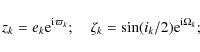
|
(2) |
for k=b,c,d, we have for the linear Laplace-Lagrange solution
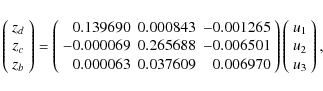
where the proper modes uk are obtained from the zk by inverting the above linear relation. To good approximation, we then have
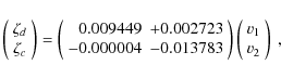
and the additional approximate relation
The proper modes in inclination are then given to a good approximation as
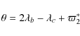
With Eq. (3),
it is then easy to understand the meaning of the observed libration
between the periastrons ![]() and
and ![]() .
Indeed, for both planets b and c,
the dominant term is the u2
term with frequency g2. They
thus both precess with an average value of g2.
In the same way, both nodes
.
Indeed, for both planets b and c,
the dominant term is the u2
term with frequency g2. They
thus both precess with an average value of g2.
In the same way, both nodes ![]() and
and ![]() precess with the same frequency s2.
It should also be noted that Eqs. (3)-(5)
provide good approximations of the long-term evolution of the
eccentricities and inclinations. Indeed, in Fig. 5 we plot the
eccentricity and the inclination with respect to the invariant plane of
planets b, c, d,
with initial conditions from Table 2. At the same time, we
plot with solid black lines the evolution of the same elements given by
the above secular, linear approximation.
precess with the same frequency s2.
It should also be noted that Eqs. (3)-(5)
provide good approximations of the long-term evolution of the
eccentricities and inclinations. Indeed, in Fig. 5 we plot the
eccentricity and the inclination with respect to the invariant plane of
planets b, c, d,
with initial conditions from Table 2. At the same time, we
plot with solid black lines the evolution of the same elements given by
the above secular, linear approximation.
The eccentricity and inclination variations are very limited
and described well by the secular approximation. The eccentricity of
planets b and c are within the
ranges 0.028 < eb
< 0.050 and
0.258 < ec
< 0.279, respectively. These variations are driven mostly by the
rapid secular frequency g3 -
g2, of period ![]() yr
(Table 4).
The eccentricity of planet d is nearly constant
with 0.136 < ed
< 0.142.
yr
(Table 4).
The eccentricity of planet d is nearly constant
with 0.136 < ed
< 0.142.
The inclinations of b and c
with respect to the invariant plane are very small with ![]() and
and ![]() ,
respectively. This small variation is mostly caused by the non-linear
secular term 2 (s2-g2)
of period 4.791 yr. Although the inclination of d
is not well constrained, using the initial conditions of Table 2, one finds small
variations in its inclination
,
respectively. This small variation is mostly caused by the non-linear
secular term 2 (s2-g2)
of period 4.791 yr. Although the inclination of d
is not well constrained, using the initial conditions of Table 2, one finds small
variations in its inclination ![]() ,
which are driven by the secular frequency s1-s2
of period 138.3 yr (Table 4).
,
which are driven by the secular frequency s1-s2
of period 138.3 yr (Table 4).
![\begin{figure}
\par\includegraphics*[width=8cm,clip]{12700fg5.ps}
\end{figure}](/articles/aa/full_html/2010/03/aa12700-09/img166.png)
|
Figure 5: Evolution of the GJ 876 eccentricities ( top) and inclinations ( bottom) with time, starting with the orbital solution from Table 2. The color lines are the complete solutions for the various planets (b: blue, c: green, d: red), while the black curves are the associated values obtained with the linear, secular model. |
| Open with DEXTER | |
With the present 11 years of observations covered by Keck and HARPS, the most important features that allow us to constrain the parameters of the system are those related to the rapid secular frequencies g2 and s2, of periods 8.7 yr and 99 yr, which are the precession frequencies of the periastrons and nodes of planets b and c.
4.2 The 2:1 mean motion resonance
Table 4: Fundamental frequencies and phases for the orbital solution in Table 2.
The ratio of the orbital periods of the two outermost planets
determined by the fitting process (Table 2) is Pb
/ Pc =
2.018, suggesting that the system may be trapped in a 2:1
mean motion resonance. This resonant motion has already been reported
in previous works
(Laughlin
& Chambers 2001; ; Rivera & Lissauer 2001;
Ji
et al. 2002; Lee & Peale 2002).
To test the accuracy of this scenario, we performed a frequency
analysis of the orbital solution listed in Table 2 computed over
100 kyr.
The orbits of the three planets are integrated with the symplectic
integrator SABA4 of Laskar
& Robutel (2001), using a step size
of ![]() years.
We conclude that in the nominal solution of Table 2,
planets b and c in the
GJ 876 system indeed show a
2:1 mean motion resonance, with resonant arguments:
years.
We conclude that in the nominal solution of Table 2,
planets b and c in the
GJ 876 system indeed show a
2:1 mean motion resonance, with resonant arguments:
![]() and
and
![]() .
.
If we analyze these arguments, it is indeed difficult to
disentangle the proper libration from the secular oscillation of the
periastrons angles ![]() .
It is thus much clearer to switch to proper modes uk,vk
by means of the linear transformation (3, 4). Indeed, if
.
It is thus much clearer to switch to proper modes uk,vk
by means of the linear transformation (3, 4). Indeed, if ![]() ,
the argument
,
the argument
is in libration around
![\begin{figure}
\par\includegraphics*[width=8.8cm,clip]{12700fg6.ps}
\end{figure}](/articles/aa/full_html/2010/03/aa12700-09/img187.png)
|
Figure 6:
Variation in the resonant argument |
| Open with DEXTER | |
Table 5:
Quasi-periodic decomposition of the resonant angle
![]() for an integration over 100 kyr of the orbital solution in
Table 2.
for an integration over 100 kyr of the orbital solution in
Table 2.
4.3 Coplanar motion
The orbits of the planets in the Solar System are nearly coplanar, that
is, their
orbital planes remain within a few degrees of inclination from an
inertial plane
perpendicular to the total angular momentum of the system. The highest
inclination is obtained for Mercury (
![]() ), which is also the smallest
of the
eight planets.
), which is also the smallest
of the
eight planets.
A general belief that planetary systems would tend to resemble the Solar System persists, but there is no particular reason for all planetary systems to be coplanar such as our own. Star formation theories require an accretion disk in which planets form, but close encounters during the formation process can increase the eccentricities and inclinations (e.g. Lee et al. 2007). That planets are found to have significant eccentricity values is also consistent with their having high inclinations (e.g. Libert & Tsiganis 2009). In particular, studies of Kuiper belt objects indicate that there is an important inclination excitation when the bodies sweep secular resonances (e.g. Nagasawa et al. 2000; Li et al. 2008), a mechanism that also appears to be applicable to planets (e.g. Thommes & Lissauer 2003).
The question of whether extra-solar planetary systems are also nearly coplanar or not is thus important. Although about 45 extra-solar multi-planet systems have been reported, their true inclinations have so far been determined in only two cases. One is the planetary system around the pulsar PSR B1257 + 12, discovered by precise timing measurements of pulses (Wolszczan & Frail 1992), for which the orbits seem to be almost coplanar (Konacki & Wolszczan 2003). The other case is GJ 876, the only planetary system around a main-sequence star for which one can access the inclinations. This result is possible because of the large amount of data already available and because the two giant planets show strong gravitational interactions.
The analytical expressions and the plots versus time of the
orbital elements in the reference frame of the invariant plane show
that the inclinations of planets b and c
are both very small (Eqs. (4),
(5),
Fig. 5).
To test the coplanarity of this system, we plot in Fig. 7 the evolution of the
mutual inclination with time.
We verify that ![]() ,
and hence conclude that
the orbits of planets b and c
are indeed nearly coplanar.
,
and hence conclude that
the orbits of planets b and c
are indeed nearly coplanar.
![\begin{figure}
\par\includegraphics*[width=9cm]{12700fg7.ps}
\end{figure}](/articles/aa/full_html/2010/03/aa12700-09/img193.png)
|
Figure 7:
Evolution of the mutual inclination of the planets b
and c. Since the maximal inclination between the
two planets is |
| Open with DEXTER | |
In our best-fit solution (Table 2),
we also assumed that the orbit of
planet d is nearly coplanar with the other two
planets, but there is no clear
physical reason that justifies our choice.
Indeed, its orbit should be more perturbed by the oblateness of the
star, rather
than the other planets (Goldreich 1965; Correia 2009).
It is therefore more likely
that planet d orbits in the equatorial plane of the
star. This plane can be identical to the orbital plane
of the outer planets or not, depending on the evolutionary process.
According to Fig. 2,
with the current HARPS precision of ![]() 1 m s-1,
we will have to wait until about 2050 to confirm an inclination close
to
1 m s-1,
we will have to wait until about 2050 to confirm an inclination close
to ![]() .
.
Adopting ![]() ,
and initial values of id
ranging from
,
and initial values of id
ranging from ![]() to
to
![]() ,
we found best-fit solutions with very similar values of reduced
,
we found best-fit solutions with very similar values of reduced ![]() as the solution in Table 2.
For inclinations lower than
as the solution in Table 2.
For inclinations lower than ![]() ,
the best-fit solution becomes worse (
,
the best-fit solution becomes worse (
![]() for
for ![]() )
and
infers low eccentricity values for planet d. In
addition, planets b and care no
longer nearly coplanar. We therefore conclude that a lower limit to the
inclination of
planet d can be set to be around
)
and
infers low eccentricity values for planet d. In
addition, planets b and care no
longer nearly coplanar. We therefore conclude that a lower limit to the
inclination of
planet d can be set to be around ![]() .
On the other hand, a lack of transit detections only allows
inclinations close
to
.
On the other hand, a lack of transit detections only allows
inclinations close
to ![]() if the planet is very dense (Rivera
et al. 2005).
if the planet is very dense (Rivera
et al. 2005).
4.4 Stability analysis
![\begin{figure}
\par\includegraphics[width=8.8cm]{12700fg8.ps}
\end{figure}](/articles/aa/full_html/2010/03/aa12700-09/img196.png)
|
Figure 8:
Stability analysis of the nominal fit (Table 2) of the
GJ 876 planetary system. For a fixed initial condition of
planet b ( left) and planet c
( right), the phase space of the system is explored
by varying the semi-major axis ak
and eccentricity ek
of the other planet, respectively. The step size is 0.0002 AU
in semi-major axis and 0.005 in eccentricity in the top panels
and |
| Open with DEXTER | |
To analyze the stability of the nominal solution (Table 2) and confirm the presence of the 2:1 resonance, we performed a global frequency analysis (Laskar 1993) in the vicinity of this solution (Fig. 4), in the same way as achieved for the HD 45364 system by Correia et al. (2009).
For each planet, the system is integrated on a regular 2D mesh of initial conditions, with varying semi-major axis and eccentricity, while the other parameters are retained at their nominal values (Table 2). The solution is integrated over 800 yr for each initial condition and a stability indicator is computed to be the variation in the measured mean motion over the two consecutive 400 yr intervals of time. For regular motion, there is no significant variation in the mean motion along the trajectory, while it can vary significantly for chaotic trajectories. The result is reported in color in Fig. 8, where ``red'' represents the strongly chaotic trajectories, and ``dark blue'' the extremely stable ones. To decrease the computation time, we averaged the orbit of planet d over its mean-motion and periastron, following Farago et al. (2009).
In the two top plots (Figs. 8a,b),
the only stable zone that exists in the vicinity of the nominal
solution corresponds to the stable 2:1 resonant areas. As for
HD 45364 (Correia
et al. 2009) and HD 60532
(Laskar & Correia
2009) planetary systems, there is a perfect coincidence
between the stable 2:1 resonant islands, and curves of minimal ![]() obtained by
comparison with the observations.
Since these islands are the only stable zones in the vicinity, this
picture presents a very coherent view of dynamical analysis and radial
velocity measurements, which reinforces the confidence that the present
system is in a 2:1 resonant state.
obtained by
comparison with the observations.
Since these islands are the only stable zones in the vicinity, this
picture presents a very coherent view of dynamical analysis and radial
velocity measurements, which reinforces the confidence that the present
system is in a 2:1 resonant state.
The scale of the two bottom panels shows the remarkable
precision of the data
in light of the dynamical environment of the system. The darker
structures in these plots can be identified as secondary resonances.
For instance, in the bottom left plot of Fig. 7, the two dark
horizontal lines
starting at ![]() and 0.260 correspond, respectively, to
and 0.260 correspond, respectively, to ![]() and
and ![]() .
We can also barely
see the secondary resonance
.
We can also barely
see the secondary resonance ![]() just above the former one.
In the bottom right plot, the bluer line starting at
just above the former one.
In the bottom right plot, the bluer line starting at ![]() corresponds
to
corresponds
to ![]() .
A longer integration time
would most probably provide more details about the resonant and secular
dynamics.
.
A longer integration time
would most probably provide more details about the resonant and secular
dynamics.
4.5 Long-term orbital evolution
![\begin{figure}
\par\includegraphics*[width=8.8cm]{12700fg9.ps}
\end{figure}](/articles/aa/full_html/2010/03/aa12700-09/img203.png)
|
Figure 9: Long-term evolution of the GJ 876 planetary system over 100 Myr starting with the orbital solution from Table 2. We did not include tidal effects in this simulation. The panel shows a face-on view of the system invariant plane. x and y are spatial coordinates in a frame centered on the star. Present orbital solutions are traced with solid lines and each dot corresponds to the position of the planet every 5 kyr. The semi-major axes (in AU) are almost constant ( 0.209 < ab < 0.214; 0.131 < ac < 0.133 and 0.02110 < ad < 0.02111), and the eccentricities present slight variations ( 0.028 < eb < 0.050; 0.258 < ec < 0.279 and 0.136 < ed < 0.142). |
| Open with DEXTER | |
![\begin{figure}
\par\includegraphics[width=14cm,clip]{12700fg0.ps}
\end{figure}](/articles/aa/full_html/2010/03/aa12700-09/img204.png)
|
Figure 10:
Possible location of an additional fourth planet in the GJ 876
system. The stability of an Earth-size planet (K=1 m s-1)
is analyzed, for various semi-major axis versus eccentricity (
top), or mean anomaly ( bottom). All the
angles of the putative planets are set to |
| Open with DEXTER | |
From the previous stability analysis, it is clear that planets b and clisted in Table 2 are trapped in a 2:1 mean motion resonance and stable over a Gyr timescale. Nevertheless, we also tested this by performing a numerical integration of the orbits using the symplectic integrator SABA4.
Because the orbital period of the innermost planet is shorter
than 2 day, we
performed two kinds of experiments.
In the first one, we directly integrated the full planetary system over
100 Myr with a step size of ![]() years.
Although tidal effects may play an important role in this system
evolution, we
did not include them.
The result is displayed in Fig. 9,
showing that the orbits indeed evolve in a regular way, and remain
stable throughout the simulation.
For longer timescales, we needed to average the orbit of the inner
planet as
explained in Farago
et al. (2009).
We then use a longer step size of
years.
Although tidal effects may play an important role in this system
evolution, we
did not include them.
The result is displayed in Fig. 9,
showing that the orbits indeed evolve in a regular way, and remain
stable throughout the simulation.
For longer timescales, we needed to average the orbit of the inner
planet as
explained in Farago
et al. (2009).
We then use a longer step size of ![]() years
and integrated the
system over 5 Gyr, which corresponds to the maximal estimated
age of
the central star. The subsystem consisting of the giant planets b
and cremained stable.
years
and integrated the
system over 5 Gyr, which corresponds to the maximal estimated
age of
the central star. The subsystem consisting of the giant planets b
and cremained stable.
In spite of the strong gravitational interactions between the
two planets locked
in the 2:1 mean motion resonance, both orbital eccentricities and
inclinations
exhibit small variations that are mostly driven by the regular linear
secular terms (Fig. 5).
These variations occur far more rapidly than in our Solar System, which
enabled
their direct detection using only 11 yr of data taken with
Keck and HARPS together.
It is important to notice, however, that
for initial inclinations of planet d very different
from ![]() ,
the
orbital perturbations from the outer planets may become important.
For instance, using an orbital solution with
,
the
orbital perturbations from the outer planets may become important.
For instance, using an orbital solution with ![]() ,
we derive an
eccentricity and inclination variations of
0.10 < ed
< 0.35 and
,
we derive an
eccentricity and inclination variations of
0.10 < ed
< 0.35 and ![]() .
.
4.6 Additional constraints
The stability analysis summarized in Fig. 8 shows good agreement
between the 2:1 resonant islands and the ![]() contour curves.
We can thus assume that the dynamics of the two known planets is not
disturbed much by the presence of an additional planet close-by.
The same is true for the innermost planet, which has an orbital period
of 2 day, since the gravitational interaction with the parent
star is too strong to be destabilized.
contour curves.
We can thus assume that the dynamics of the two known planets is not
disturbed much by the presence of an additional planet close-by.
The same is true for the innermost planet, which has an orbital period
of 2 day, since the gravitational interaction with the parent
star is too strong to be destabilized.
We then tested the possibility of an additional fourth planet in the system by varying the semi-major axis, the eccentricity, and the longitude of the periastron over a wide range, and performing a stability analysis (Fig. 10). The test was completed for a fixed value K=1 m s-1, corresponding to an Earth-size object. We also performed a simulation of a Neptune-size object (K=10 m s-1) without significant changes in its dynamics. In this last case, however, an object of this size would have already been detected in the data.
From this analysis (Fig. 10), one can see that
stable orbits are possible
beyond 1 AU and, very interestingly, also for orbital periods
around 15 days
(![]() 0.083 AU),
which correspond to bodies trapped in a 4:1 mean motion resonance
with planet b (and 2:1 resonance with planet c).
Between the already known planets, this is the only zone where
additional
planetary mass companions can survive.
With the current HARPS precision of
0.083 AU),
which correspond to bodies trapped in a 4:1 mean motion resonance
with planet b (and 2:1 resonance with planet c).
Between the already known planets, this is the only zone where
additional
planetary mass companions can survive.
With the current HARPS precision of ![]() 1 m s-1,
we estimate that any object
with a minimum mass
1 m s-1,
we estimate that any object
with a minimum mass ![]() would already be visible in the data.
Since this does not seem to be the case, if we assume that a planet
exists in
this resonant stable zone, it should be an object smaller or not much
larger than the Earth.
would already be visible in the data.
Since this does not seem to be the case, if we assume that a planet
exists in
this resonant stable zone, it should be an object smaller or not much
larger than the Earth.
The presence of this fourth planet, not only fills an empty
gap in the
system, but can also help us to explain the anomalous high eccentricity
of planet d (
![]() ). Indeed, tidal interactions
with the star should have circularized the orbit in less than
1 Myr, but according to Mardling
(2007), the presence of an Earth-sized outer planet may delay
the tidal damping of the eccentricity.
). Indeed, tidal interactions
with the star should have circularized the orbit in less than
1 Myr, but according to Mardling
(2007), the presence of an Earth-sized outer planet may delay
the tidal damping of the eccentricity.
We propose that additional observational efforts should be made to search for this planet. The orbital period of only 15 day does not require long time of telescope and a planet with the mass of the Earth is at reach with the present resolution. Moreover, assuming coplanar motion with the outermost planets, we obtain the exact mass for this planet and not a minimal estimation. We have reanalyzed the residuals of the system (Fig. 3), but so far no signal around 15 days appears to be present with the current precision. However, since this planet will be in a 2:1 mean motion resonance with planet c, we cannot exclude that the signal is hidden in the eccentricity of the giant planet (Anglada-Escude et al. 2010).
5 Discussion and conclusion
We have reanalyzed the planetary system orbiting the star
GJ 876, using
the new high-precision observational data acquired with HARPS.
Independently from previous observations with other instruments, we can
confirm
the presence of planet d, orbiting at 1.93785 days,
but in an elliptical orbit with an eccentricity of 0.14 and a minimum
mass of ![]() .
.
By combining the HARPS data with the data previously taken at
the
Keck Observatory, we are able to fully characterize the b
and cplanets. We find ![]() and
and ![]() ,
which infers for the true masses of the planets
,
which infers for the true masses of the planets ![]() and
and ![]() ,
respectively. We hence conclude that the orbits of these two planets
are nearly coplanar.
The gravitational interactions between the outer planets and the
innermost planet d may also allow us to determine
its orbit more accurately
in the near future. With the current precision of HARPS of
,
respectively. We hence conclude that the orbits of these two planets
are nearly coplanar.
The gravitational interactions between the outer planets and the
innermost planet d may also allow us to determine
its orbit more accurately
in the near future. With the current precision of HARPS of ![]() 1 m s-1
for GJ 876, we expect to detect the true inclination and mass
of planet d within some decades.
1 m s-1
for GJ 876, we expect to detect the true inclination and mass
of planet d within some decades.
A dynamical analysis of this planetary system confirms that
planets b and care locked in a
2:1 mean motion resonance, which ensures stability over 5 Gyr.
In the nominal solution, the resonant angles ![]() and
and ![]() are
in libration around
are
in libration around ![]() ,
which means that their periastrons are
also aligned.
This orbital configuration may have been reached by means of the
dissipative
process of planet migration during the early stages of the system
evolution
(e.g. Crida et al.
2008). By analyzing the proper modes, we are able to see that
the amplitude libration of the proper resonant argument
,
which means that their periastrons are
also aligned.
This orbital configuration may have been reached by means of the
dissipative
process of planet migration during the early stages of the system
evolution
(e.g. Crida et al.
2008). By analyzing the proper modes, we are able to see that
the amplitude libration of the proper resonant argument ![]() can be as small as
can be as small as ![]() ,
of which only
,
of which only ![]() is related to the libration frequency. It is thus remarkable that the
libration amplitude is so small, owing to the width of the stable
resonant island being large. We can thus assume that the libration
amplitude has been damped by some dissipative process. This singular
planetary system may then provide important constraints on planetary
formation and migration scenarios.
is related to the libration frequency. It is thus remarkable that the
libration amplitude is so small, owing to the width of the stable
resonant island being large. We can thus assume that the libration
amplitude has been damped by some dissipative process. This singular
planetary system may then provide important constraints on planetary
formation and migration scenarios.
Finally, we have found that stability is possible for an
Earth-size mass planet
or smaller in an orbit around 15 days, which is in a 4:1 mean
motion resonance
with planet b.
The presence of this fourth planet, not only fills an empty gap in the
system, but can also help us to explain the anomalous high eccentricity
of planet d (
![]() ), which should have been
damped to zero by tides.
Because of the proximity and low mass of the star, a planet with the
mass of the Earth should be detectable at the present HARPS resolution.
), which should have been
damped to zero by tides.
Because of the proximity and low mass of the star, a planet with the
mass of the Earth should be detectable at the present HARPS resolution.
We conclude that the radial-velocity technique is self sufficient for fully characterizing and determining all the orbital parameters of a multi-planet system, without needing to use astrometry or transits.
AcknowledgementsWe acknowledge support from the Swiss National Research Found (FNRS), the Geneva University and French CNRS. A.C. also benefited from a grant by the Fundação para a Ciência e a Tecnologia, Portugal (PTDC/CTE-AST/098528/2008).
References
- Anglada-Escude, G., Lopez-Morales, M., & Chambers, J. E. 2010, ApJ, 709, 168 [NASA ADS] [CrossRef] [Google Scholar]
- Bean, J. L., & Seifahrt, A. 2009, A&A, 496, 249 [NASA ADS] [CrossRef] [EDP Sciences] [MathSciNet] [Google Scholar]
- Beaugé, C., Ferraz-Mello, S., & Michtchenko, T. A. 2003, ApJ, 593, 1124 [Google Scholar]
- Benedict, G. F., McArthur, B. E., Forveille, T., et al. 2002, ApJ, 581, L115 [NASA ADS] [CrossRef] [Google Scholar]
- Bonfils, X., Delfosse, X., Udry, S., et al. 2005a, A&A, 442, 635 [NASA ADS] [CrossRef] [EDP Sciences] [Google Scholar]
- Bonfils, X., Forveille, T., Delfosse, X., et al. 2005b, A&A, 443, L15 [NASA ADS] [CrossRef] [EDP Sciences] [Google Scholar]
- Bonfils, X., Mayor, M., Delfosse, X., et al. 2007, A&A, 474, 293 [NASA ADS] [CrossRef] [EDP Sciences] [Google Scholar]
- Correia, A. C. M. 2009, ApJ, 704, L1 [NASA ADS] [CrossRef] [Google Scholar]
- Correia, A. C. M., Udry, S., Mayor, M., et al. 2005, A&A, 440, 751 [NASA ADS] [CrossRef] [EDP Sciences] [Google Scholar]
- Correia, A. C. M., Udry, S., Mayor, M., et al. 2009, A&A, 496, 521 [NASA ADS] [CrossRef] [EDP Sciences] [Google Scholar]
- Crida, A., Sándor, Z., & Kley, W. 2008, A&A, 483, 325 [NASA ADS] [CrossRef] [EDP Sciences] [Google Scholar]
- Cutri, R. M., Skrutskie, M. F., van Dyk, S., et al. 2003, 2MASS All Sky Catalog of point sources, The IRSA 2MASS All-Sky Point Source Catalog, NASA/IPAC Infrared Science Archive http://irsa.ipac.caltech.edu/applications/Gator/ [Google Scholar]
- Delfosse, X., Forveille, T., Mayor, M., et al. 1998, A&A, 338, L67 [Google Scholar]
- Delfosse, X., Forveille, T., Ségransan, D., et al. 2000, A&A, 364, 217 [NASA ADS] [Google Scholar]
- ESA 1997, VizieR Online Data Catalog, 1239 [Google Scholar]
- Farago, F., Laskar, J., & Couetdic, J. 2009, Celestial Mechanics and Dynamical Astronomy, 104, 291 [NASA ADS] [CrossRef] [Google Scholar]
- Forveille, T., Bonfils, X., Delfosse, X., et al. 2009, A&A, 493, 645 [NASA ADS] [CrossRef] [EDP Sciences] [Google Scholar]
- Goldreich, P. 1965, AJ, 70, 5 [NASA ADS] [CrossRef] [Google Scholar]
- Hawley, S. L., Gizis, J. E., & Reid, I. N. 1996, AJ, 112, 2799 [NASA ADS] [CrossRef] [Google Scholar]
- Henry, T. J., & McCarthy, Jr., D. W. 1993, AJ, 106, 773 [NASA ADS] [CrossRef] [Google Scholar]
- Ji, J., Li, G., & Liu, L. 2002, ApJ, 572, 1041 [NASA ADS] [CrossRef] [Google Scholar]
- Johnson, J. A., & Apps, K. 2009, ApJ, 699, 933 [NASA ADS] [CrossRef] [Google Scholar]
- Konacki, M., & Wolszczan, A. 2003, ApJ, 591, L147 [NASA ADS] [CrossRef] [Google Scholar]
- Kürster, M., Endl, M., Rouesnel, F., et al. 2003, A&A, 403, 1077 [NASA ADS] [CrossRef] [EDP Sciences] [Google Scholar]
- Laskar, J. 1990, Icarus, 88, 266 [NASA ADS] [CrossRef] [Google Scholar]
- Laskar, J. 1993, Physica D Nonlinear Phenomena, 67, 257 [Google Scholar]
- Laskar, J., & Correia, A. C. M. 2009, A&A, 496, L5 [NASA ADS] [CrossRef] [EDP Sciences] [Google Scholar]
- Laskar, J., & Robutel, P. 2001, Celestial Mechanics and Dynamical Astronomy, 80, 39 [NASA ADS] [CrossRef] [Google Scholar]
- Laughlin, G., & Chambers, J. E. 2001, ApJ, 551, L109 [NASA ADS] [CrossRef] [Google Scholar]
- Lee, M. H., & Peale, S. J. 2002, ApJ, 567, 596 [NASA ADS] [CrossRef] [Google Scholar]
- Lee, M. H., Peale, S. J., Pfahl, E., et al. 2007, Icarus, 190, 103 [NASA ADS] [CrossRef] [Google Scholar]
- Leggett, S. K. 1992, ApJS, 82, 351 [NASA ADS] [CrossRef] [Google Scholar]
- Leggett, S. K., Allard, F., Geballe, T. R., Hauschildt, P. H., & Schweitzer, A. 2001, ApJ, 548, 908 [NASA ADS] [CrossRef] [Google Scholar]
- Li, J., Zhou, L.-Y., & Sun, Y.-S. 2008, Chin. Astron. Astrophys., 32, 409 [Google Scholar]
- Libert, A.-S., & Tsiganis, K. 2009, A&A, 493, 677 [NASA ADS] [CrossRef] [EDP Sciences] [Google Scholar]
- Marcy, G. W., Butler, R. P., Vogt, S. S., Fischer, D., & Lissauer, J. J. 1998, ApJ, 505, L147 [NASA ADS] [CrossRef] [Google Scholar]
- Marcy, G. W., Butler, R. P., Fischer, D., et al. 2001, ApJ, 556, 296 [NASA ADS] [CrossRef] [Google Scholar]
- Mardling, R. A. 2007, MNRAS, 382, 1768 [NASA ADS] [Google Scholar]
- Mayor, M., Pepe, F., Queloz, D., et al. 2003, The Messenger, 114, 20 [NASA ADS] [Google Scholar]
- Mayor, M., Bonfils, X., Forveille, T., et al. 2009, A&A, 507, 487 [NASA ADS] [CrossRef] [EDP Sciences] [Google Scholar]
- Nagasawa, M., Tanaka, H., & Ida, S. 2000, AJ, 119, 1480 [NASA ADS] [CrossRef] [Google Scholar]
- Press, W. H., Teukolsky, S. A., Vetterling, W. T., et al. 1992, Numerical recipes in FORTRAN, 2nd edn. The art of scientific computing (Cambridge: University Press) [Google Scholar]
- Rivera, E. J., & Lissauer, J. J. 2001, ApJ, 558, 392 [NASA ADS] [CrossRef] [MathSciNet] [Google Scholar]
- Rivera, E. J., Lissauer, J. J., Butler, R. P., et al. 2005, ApJ, 634, 625 [NASA ADS] [CrossRef] [Google Scholar]
- Thommes, E. W., & Lissauer, J. J. 2003, ApJ, 597, 566 [NASA ADS] [CrossRef] [Google Scholar]
- Turon, C., Creze, M., Egret, D., et al. 1993, Bulletin d'Information du Centre de Données Stellaires, 43, 5 [Google Scholar]
- Udry, S., Bonfils, X., Delfosse, X., et al. 2007, A&A, 469, L43 [NASA ADS] [CrossRef] [EDP Sciences] [Google Scholar]
- Wolszczan, A., & Frail, D. A. 1992, Nature, 355, 145 [NASA ADS] [CrossRef] [Google Scholar]
Footnotes
- ... system
- Based on observations made with the HARPS instrument on the ESO 3.6 m telescope at La Silla Observatory under the GTO programme ID 072.C-0488; and on observations obtained at the Keck Observatory, which is operated jointly by the University of California and the California Institute of Technology.
- ...
- The Table with the HARPS radial velocities is only available in electronic form at the CDS via anonymous ftp to
cdsarc.u-strasbg.fr (130.79.128.5) or via http://cdsweb.u-strasbg.fr/cgi-bin/qcat?J/A+A/511/A21 - ...
system
- http://www.chara.gsu.edu/RECONS/TOP100.posted.htm
All Tables
Table 1: Observed and inferred stellar parameters of GJ 876.
Table 2: Orbital parameters for the planets orbiting GJ 876, obtained with a 4-body Newtonian fit to observational data from Keck and HARPS.
Table 3: Orbital parameters for the planets orbiting GJ 876, obtained with a 4-body Newtonian fit to all available radial velocity observational data (Lick, Keck, CORALIE, ELODIE, and HARPS).
Table 4: Fundamental frequencies and phases for the orbital solution in Table 2.
Table 5:
Quasi-periodic decomposition of the resonant angle
![]() for an integration over 100 kyr of the orbital solution in
Table 2.
for an integration over 100 kyr of the orbital solution in
Table 2.
All Figures
|
|
Figure 1: Keck and HARPS radial velocities for GJ 876, superimposed on the 3-body Newtonian (two planets) orbital solution for planets b and c (orbital parameters taken from Table 2). |
| Open with DEXTER | |
| In the text | |
|
|
Figure 2: Frequency analysis and window function for the two-planet Keck and HARPS residual radial velocities of GJ 876 (Fig. 1). An important peak is detected at P = 1.9379 day, which can be interpreted as a third planetary companion in the system. Looking at the window function, we can see that this peak is not an artifact. |
| Open with DEXTER | |
| In the text | |
|
|
Figure 3: Phase-folded residual radial velocities for GJ 876 when the contributions from the planets b and c are subtracted. Data are superimposed on a Keplerian orbit of P = 1.9378 day and e = 0.14 (the complete set of orbital parameters are those from Table 2). The respective residuals as a function of Julian date are displayed in the lower panel. |
| Open with DEXTER | |
| In the text | |
|
|
Figure 4:
Radial velocity differences between orbital solutions with |
| Open with DEXTER | |
| In the text | |
|
|
Figure 5: Evolution of the GJ 876 eccentricities ( top) and inclinations ( bottom) with time, starting with the orbital solution from Table 2. The color lines are the complete solutions for the various planets (b: blue, c: green, d: red), while the black curves are the associated values obtained with the linear, secular model. |
| Open with DEXTER | |
| In the text | |
|
|
Figure 6:
Variation in the resonant argument |
| Open with DEXTER | |
| In the text | |
|
|
Figure 7:
Evolution of the mutual inclination of the planets b
and c. Since the maximal inclination between the
two planets is |
| Open with DEXTER | |
| In the text | |
|
|
Figure 8:
Stability analysis of the nominal fit (Table 2) of the
GJ 876 planetary system. For a fixed initial condition of
planet b ( left) and planet c
( right), the phase space of the system is explored
by varying the semi-major axis ak
and eccentricity ek
of the other planet, respectively. The step size is 0.0002 AU
in semi-major axis and 0.005 in eccentricity in the top panels
and |
| Open with DEXTER | |
| In the text | |
|
|
Figure 9: Long-term evolution of the GJ 876 planetary system over 100 Myr starting with the orbital solution from Table 2. We did not include tidal effects in this simulation. The panel shows a face-on view of the system invariant plane. x and y are spatial coordinates in a frame centered on the star. Present orbital solutions are traced with solid lines and each dot corresponds to the position of the planet every 5 kyr. The semi-major axes (in AU) are almost constant ( 0.209 < ab < 0.214; 0.131 < ac < 0.133 and 0.02110 < ad < 0.02111), and the eccentricities present slight variations ( 0.028 < eb < 0.050; 0.258 < ec < 0.279 and 0.136 < ed < 0.142). |
| Open with DEXTER | |
| In the text | |
|
|
Figure 10:
Possible location of an additional fourth planet in the GJ 876
system. The stability of an Earth-size planet (K=1 m s-1)
is analyzed, for various semi-major axis versus eccentricity (
top), or mean anomaly ( bottom). All the
angles of the putative planets are set to |
| Open with DEXTER | |
| In the text | |
Copyright ESO 2010
Current usage metrics show cumulative count of Article Views (full-text article views including HTML views, PDF and ePub downloads, according to the available data) and Abstracts Views on Vision4Press platform.
Data correspond to usage on the plateform after 2015. The current usage metrics is available 48-96 hours after online publication and is updated daily on week days.
Initial download of the metrics may take a while.