| Issue |
A&A
Volume 511, February 2010
|
|
|---|---|---|
| Article Number | A17 | |
| Number of page(s) | 8 | |
| Section | Astrophysical processes | |
| DOI | https://doi.org/10.1051/0004-6361/200912669 | |
| Published online | 24 February 2010 | |
Resonant absorption with 2D variation of field line eigenfrequencies
A. J. B. Russell - A. N. Wright
School of Mathematics and Statistics, University of St Andrews, North Haugh, St Andrews, Fife KY16 9SS, Scotland, UK
Received 9 June 2009 / Accepted 13 December 2009
Abstract
Context. Resonant absorption, also known as field line
resonance, can be used to describe coupling between fast and Alfvén
waves in non-uniform plasmas. Since the conditions for resonant
absorption occur widely in astrophysics, it is applicable in many
different contexts, all of which are united by their common physics.
For example, resonant absorption is known to play a major role in the
excitation of ultra-low frequency pulsations in the terrestrial
magnetosphere and is also a leading explanation for the decay of fast
kink oscillations of coronal loops. The occurrence of non-axisymmetric
conditions in the magnetosphere, and observational evidence that
coronal loops may possess fine transverse structure, highlight a need
to consider equilibria that vary in two dimensions across the
background magnetic field.
Aims. We investigate the properties of resonant absorption when
field line eigenfrequencies vary in two dimensions across the
background magnetic field. We aim to place the theory on a firm
mathematical footing and explore some of its key features.
Methods. Using cold, linear, ideal MHD with a straight, uniform
background magnetic field, we systematically obtain a complete analytic
solution for behaviour at late times. This provides a framework from
which the features of resonant absorption may be understood. The
time-dependent problem is solved numerically, reproducing key features
of the analytic solution.
Results. Energy is deposited from a monochromatic fast wave as a
phase mixing Alfvén wave, in the vicinity of the resonant surface, at
which the local field line eigenfrequency matches the frequency of the
driver. A generalisation of the one dimensional phase mixing length to
higher dimensions is suggested, and shown to successfully estimate the
finest lengthscales in time-dependent simulations. The resonant Alfvén
wave is driven by gradients of the field aligned magnetic field
perturbation, which is associated with the fast wave pressure. This
leads to amplitude variations of the Alfvén wave that can be used to
reveal the spatial form of the fast wave.
Key words: magnetohydrodynamics (MHD) - waves - magnetic fields - Sun: oscillations - Sun: corona - Earth
1 Introduction
Resonant absorption, also known as field line resonance, can be used to describe the transfer of energy between fast magnetoacoustic and Alfvén waves in non-uniform plasmas. By combining the different properties of these two waves, this fundamental process opens new paths for energy to flow through astrophysical systems.The basic requirements for resonant absorption are a source of compressive energy such as global oscillations, stellar winds or non-steady accretion flows, and gradients in magnetic field or plasma density. These occur widely in astrophysics. The mechanism of resonant absorption is generic, so it is reasonable to expect it to occur across a wide range of scenarios. Here, we focus on the physics of resonant absorption, but, for illustration, we will place our work in the context of two systems in which it is already believed to play a key role: the origin of ultra-low frequency (ULF) geomagnetic pulsations in the terrestrial magnetosphere; and the decay of fast kink oscillations of coronal loops. In addition, Rezania & Samson (2005) recently explained periodic oscillations in X-ray flux from an accreting neutron star in terms of resonant absorption, providing a good example of its wider application to non-heliospheric bodies.
ULF pulstations are magnetic waves at mHz frequencies that have been observed from the surface of the Earth since the Carrington event in 1859 (Stewart 1861). The ground measurements are the effect of standing Alfvén waves in the magnetosphere (Dungey 1955; Singer et al. 1982). The excitation of these waves remained a mystery until Southwood (1974) and Chen & Hasegawa (1974) independently demonstrated that resonant absorption can gradually pump energy into Alfvén waves of increasingly large amplitude from low amplitude fast waves. The ultimate energy source is the solar wind, which excites fast waves in the magnetosphere by a variety of mechanisms. Buffeting of the magnetospheric cavity preferentially excites the fast eigenmodes of the cavity, leading to the appearance of discrete frequencies (Kivelson & Southwood 1985). Kelvin-Helmholtz instability of the magnetopause provides a monochromatic source of fast waves (Mann et al. 1999). Finally, a density perturbation running along the magnetopause also produces its own fast wave signatures (Wright & Rickard 1995). Recently, magnetic pulsations have been used as a diagnostic to probe the properties of the magnetosphere (Menk et al. 1999; Mann & Wright 1999).
In coronal seismology, it was evident from the first observations of impulsively excited kink oscillations (Nakariakov et al. 1999; Aschwanden et al. 1999) that the rapid decay of these waves was not accounted for. Several explanations have been suggested, and resonant absorption is a leading candidate. In coronal loop geometries, the total pressure perturbation of the kink mode acts as a fast eigenmode of the system and couples to a resonant Alfvén wave. The wave energy, initially in the kink wave, is deposited into azimuthal motions, and the amplitude of the kink mode decays (see, e.g., Hollweg & Yang 1988; Goossens et al. 1992; Ruderman & Roberts 2002; Terradas et al. 2006, and references therein).
The structure of the magnetosphere and of coronal loops motivates consideration of resonant absorption in equilibria that vary in two dimensions across the background magnetic field. In the magnetosphere, Alfvén speed is not axisymmetric for the dawn flank, magnetotail or dusk flank, although observations show that resonant absorption persists in these regions (Takahashi et al. 1996; Anderson et al. 1990; Takahashi & Anderson 1992). Similarly, coronal loops may have non-circular cross-section (Ruderman 2003). Furthermore, there is good evidence that loops have substructure, consisting of elemental magnetic flux strands of widths less than 2 Mm (Schmelz et al. 2003; Aschwanden 2005; Schmelz et al. 2005; Schmelz 2002; Aschwanden & Nightingale 2005; Martens et al. 2002; Schmelz et al. 2001).
Investigation of resonant absorption started with consideration of a 1D density variation perpendicular to a uniform magnetic field (Chen & Hasegawa 1974; Southwood 1974). Since then, analytic efforts have been made to relax the geometric constraints of the first papers. Notably, Schulze-Berge et al. (1992) allowed the density profile to vary in three dimensions. They showed the existence of a singular solution on magnetic surfaces at which field line eigenfrequency matches the driving frequency. The leading order singular solution was obtained, but the authors stopped short of the full solution. Thompson & Wright (1993) considered a density profile that varied in one dimension across the background magnetic field and a second dimension along it. Full solutions were obtained systematically, confirming that resonant Alfvén waves are excited on field lines whose eigenfrequency matches the driver. They also demonstrated the existence of an overlap integral that determines the efficiency of the excitation: excitation is most efficient when the spatial form of the driver matches the eigenmode of the resonant field lines.
We consider a complementary problem, in which the density profile varies in two dimensions across a straight, uniform equilibrium magnetic field. This produces a 2D variation of field line eigenfrequencies, and we investigate the effect of this on resonant absorption. Numerical simulations of the initial value problem have been performed by Lee et al. (2000) and Terradas et al. (2008). These demonstrated persistence of resonant absorption for the type of equilibria considered here, and have aided qualitative understanding of its properties. A complete understanding, however, requires a mathematical solution from which key features can be teased.
This paper is organised as follows. Section 2 presents our model, with governing equations obtained in Sect. 3. Section 4 describes the numerical solutions. These show that resonant absorption is robust, the phase mixing length can be generalised to higher dimensions, and amplitude variations of the resonant Alfvén wave can be used to reveal the spatial form of the fast wave. In Sect. 5, we systematically obtain a complete analytic solution for late times. This confirms the presence of a (singular) resonant Alfvén wave, and provides insight into the relationship between amplitude variations of the resonant Alfvén wave and the spatial form of the fast wave.
2 Model
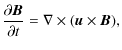
We consider an equilibrium in which the magnetic field is straight and uniform. The density varies in two dimensions perpendicular to the field. The equilibrium is maintained by the assumption that the plasma is cold, so that there is zero gas pressure (this has the additional advantage of setting the slow magnetoacoustic speed to zero, eliminating the slow wave). Gravity is neglected and we limit ourselves to times at which dissipative and non-linear effects may be considered unimportant.
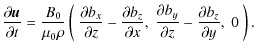
Taking the direction of the background magnetic field as an ignorable coordinate,
![]() ,
means that field line eigenfunctions are Fourier modes with an
,
means that field line eigenfunctions are Fourier modes with an ![]() ik) dependence. In an infinite medium, any value of kz may be considered. It is, however, more realistic to include boundary conditions such as line-tying, which quantises kz so that
ik) dependence. In an infinite medium, any value of kz may be considered. It is, however, more realistic to include boundary conditions such as line-tying, which quantises kz so that
![]() ,
where L is the length of the field line and n is an integer. The corresponding field line eigenfrequency is
,
where L is the length of the field line and n is an integer. The corresponding field line eigenfrequency is
![]() ,
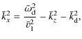
where
,
where
![]() is the Alfvén speed.
is the Alfvén speed.
We simplify matters further by specifying our driver to also have an ![]()
![]() dependence.
Since Fourier modes are orthogonal, this means that only one
eigenfunction may be driven on any field line. We therefore follow a
normal mode analysis.
dependence.
Since Fourier modes are orthogonal, this means that only one
eigenfunction may be driven on any field line. We therefore follow a
normal mode analysis.
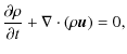
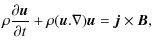
3 Governing equations
![\begin{figure}
\par\includegraphics[width=8.2cm,clip]{12669fg1.eps}
\end{figure}](/articles/aa/full_html/2010/03/aa12669-09/img25.png)
|
Figure 1: Sketch of numerical domain showing boundary conditions. |
| Open with DEXTER | |
|
(1) | ||
|
(2) | ||
|
(3) | ||
| (4) | |||
| (5) |
Taking
|
(7) |
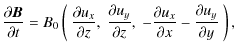
As matters stand ux, uy, bx, by and bz are functions of x, y, z and t. We consider perfectly reflecting boundaries in the z-direction (equivalent to a perfectly conducting ionosphere in a magnetospheric model), allowing us to take Fourier modes in the z direction. Writing
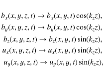
the problem reduces to 2D with governing equations


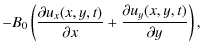

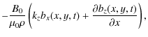

equivalent to the equations solved by Lee et al. (2000) and Terradas et al. (2008).
4 Numerical solution
4.1 Method
Before solving the governing equations numerically, we non-dimensionalised, using
| (13) | |
| (14) | |
| (15) | |
| (16) |
where u0 is the Alfvén speed at
The equations were solved with the leapfrog trapezoidal scheme detailed in Rickard & Wright (1994).
Using centred differences for spatial derivatives, this gives a code
that is second order in space and time. Boundary conditions were chosen
so that the numerical domain represents the dusk flank of the
terrestrial magnetosphere. Whilst this means that the simulation is set
up in a specific context, the essential physics remains common to all
space plasmas. The antisunward boundary at large ![]() is open to model the tail and reflections from this boundary were
avoided by advancing it ahead of all perturbations. The boundary
condition at
is open to model the tail and reflections from this boundary were
avoided by advancing it ahead of all perturbations. The boundary
condition at ![]() is symmetric, representing the nose of the magnetosphere. Most fast
waves propagating towards Earth are turned around by refraction and
redirected towards the magnetopause, so a reflecting boundary was
placed at
is symmetric, representing the nose of the magnetosphere. Most fast
waves propagating towards Earth are turned around by refraction and
redirected towards the magnetopause, so a reflecting boundary was
placed at ![]() .
Finally, the boundary at
.
Finally, the boundary at ![]() was chosen as the magnetopause and may be reflecting or driven.
was chosen as the magnetopause and may be reflecting or driven.
We used a continuous monochromatic driver. A nonuniform system supports collective modes of oscillation with discrete eigenfrequencies. When such a system is driven by a broadband source that includes one or more of its eigenfrequencies, interference leads to the dominance of those frequencies. Thus, a broadband driver drives resonances as if it were a superposition of monochromatic drivers (Kivelson & Southwood 1985; Rickard & Wright 1994; de Groof et al. 1998).
The fast wave was driven by setting ![]() at
at ![]() .
At this boundary, the displacement in the
.
At this boundary, the displacement in the ![]() direction is a sinusoidal function ramped in
direction is a sinusoidal function ramped in ![]() and
and ![]() .
This produces a function that is continuous and differentiable in
.
This produces a function that is continuous and differentiable in ![]() and
and ![]() ,
with no net displacement of the boundary over one period. Initially, the amplitude of the displacement ramps up globally over Nt
periods; under this envelope, the displacement is a sinusoidal wave
that ramps up spatially over one wavelength, is at full amplitude for Ny wavelengths and ramps down over one wavelength. Differentiating the displacement in time to obtain a velocity, we set
,
with no net displacement of the boundary over one period. Initially, the amplitude of the displacement ramps up globally over Nt
periods; under this envelope, the displacement is a sinusoidal wave
that ramps up spatially over one wavelength, is at full amplitude for Ny wavelengths and ramps down over one wavelength. Differentiating the displacement in time to obtain a velocity, we set
|
(17) |
where
|
(18) |
with
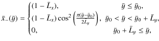
The density profile was chosen so that
![]() decreases with increasing
decreases with increasing ![]() (Alfvén speed drops off with increasing altitude in the outer
magnetosphere) and to provide a 2D variation in field line
eigenfrequencies. With these aims we chose
(Alfvén speed drops off with increasing altitude in the outer
magnetosphere) and to provide a 2D variation in field line
eigenfrequencies. With these aims we chose
|
(19) |
where
|
(20) |
and
![\begin{figure}
\par\includegraphics[width=7.2cm,clip]{12669fg2.eps}
\end{figure}](/articles/aa/full_html/2010/03/aa12669-09/img81.png)
|
Figure 2:
Cut in
|
| Open with DEXTER | |
Runs were performed with a gridspacing
![]() and a timestep
and a timestep
![]() .
For each run, the gridspacing was chosen to ensure the fine scales
produced by phase mixing were resolved with at least five points.
The code preserves energy (total energy density in the waveguide agrees
with the time integrated Poynting flux to within 0.0447% after early
times) and maintains a small
.
For each run, the gridspacing was chosen to ensure the fine scales
produced by phase mixing were resolved with at least five points.
The code preserves energy (total energy density in the waveguide agrees
with the time integrated Poynting flux to within 0.0447% after early
times) and maintains a small
![]() (the maximum value in the runs shown here was
(the maximum value in the runs shown here was
![]() ). Test cases showed that the code captures refraction of wavefronts and their reflection at boundaries in
). Test cases showed that the code captures refraction of wavefronts and their reflection at boundaries in ![]() .
As a final test, running the code with the drivers and density profile of Rickard & Wright (1994) reproduced their results.
.
As a final test, running the code with the drivers and density profile of Rickard & Wright (1994) reproduced their results.
4.2 Results
4.2.1 Excitation of resonant Alfvén wave
As a simulation runs, energy propagates throughout the domain. Since we are considering a cold plasma, features of energy density that move across magnetic field lines correspond to the fast wave. This fast wave soon reaches a quasi-steady state in the vicinity of the driven boundary, in which energy losses to the resonant Alfvén wave and flux down the waveguide approximately match energy fed in from the driven boundary.
The Alfvén speed profile means that field lines in our domain have eigenfrequencies that lie in a continuum
![]() .
When the driving frequency,
.
When the driving frequency,
![]() ,
falls outwith this continuum there is no (singular) resonant
absorption. However, when the driving frequency lies within this
continuum, energy is deposited in the vicinity of the contour at which
,
falls outwith this continuum there is no (singular) resonant
absorption. However, when the driving frequency lies within this
continuum, energy is deposited in the vicinity of the contour at which
![]() (Fig. 3).
This energy is trapped on any given field line, and the dominant
velocity perturbation is parallel to the contour. This allows us to
identify the deposited energy with the resonant Alfvén wave.
(Fig. 3).
This energy is trapped on any given field line, and the dominant
velocity perturbation is parallel to the contour. This allows us to
identify the deposited energy with the resonant Alfvén wave.
![\begin{figure}
\par\includegraphics[width=14.5cm,clip]{12669fg3.eps}
\end{figure}](/articles/aa/full_html/2010/03/aa12669-09/img91.png)
|
Figure 3:
Accumulation of energy density at a fully 2D resonant contour.
Plots show filled contours of energy density with contours representing |
| Open with DEXTER | |
4.2.2 Phase mixing
![\begin{figure}
\par\includegraphics[width=15cm,clip]{12669fg4.eps}
\end{figure}](/articles/aa/full_html/2010/03/aa12669-09/img94.png)
|
Figure 4: Phase mixing of velocity
component parallel to resonant contour. The plot is made along a curve
that is everywhere prependicular to contours of
|
| Open with DEXTER | |
|
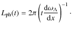
(21) |
We surmise that this result might be extended to higher dimensions by taking
| (22) |
which is in good agreement with the fine scales observed in the simulations (see the horizontal line segments indicated in Fig. 4).
4.2.3 Amplitude variations of resonant Alfvén wave revealing spatial form of fast wave
At any time, the amplitude of the resonant Alfvén wave varies
significantly along the resonant contour and the associated velocity
perturbation, ![]() ,
may change sign. (
,
may change sign. (![]() is the coordinate parallel to contours of
is the coordinate parallel to contours of
![]() and has a scale factor
and has a scale factor ![]() .) This amplitude correlates well with the magnetic pressure force associated with the fast wave
.) This amplitude correlates well with the magnetic pressure force associated with the fast wave ![]()
![]() where
where
![]() is distance along the resonant contour (Fig. 5).
The amplitude variations of the resonant Alfvén wave can therefore
reveal the spatial form of the fast wave. This relationship is
discussed more fully in Sect. 5.
is distance along the resonant contour (Fig. 5).
The amplitude variations of the resonant Alfvén wave can therefore
reveal the spatial form of the fast wave. This relationship is
discussed more fully in Sect. 5.
We further investigated cases in which field line eigenfrequencies were quasi-1D (
![]() varies little with
varies little with ![]() ,
over the wavelength of the driver). In this limit, the spatial form of
the fast wave on the resonant contour, is most strongly determined by
the wavenumber
,
over the wavelength of the driver). In this limit, the spatial form of
the fast wave on the resonant contour, is most strongly determined by
the wavenumber
![]() in the uniform region next to the driven boundary. We can set
in the uniform region next to the driven boundary. We can set
![]() in this region by varying
in this region by varying ![]() and
and
![]() ,
since
,
since
|
(23) |
for
For these cases, the relationship between the spatial form of the fast
wave and the amplitude of the resonant Alfvén wave may be seen
qualitatively in surface plots of energy density. Figure 6 shows two such plots at
![]() .
In each plot, the largest values of energy density lie on the resonant
contour and are associated with the resonant Alfvén wave. Both plots
show a foreground of fast wave energy, which lies between the resonance
and the driven boundary. In the snapshot for
.
In each plot, the largest values of energy density lie on the resonant
contour and are associated with the resonant Alfvén wave. Both plots
show a foreground of fast wave energy, which lies between the resonance
and the driven boundary. In the snapshot for
![]() ,
the Alfvén wave has been driven to sufficiently large amplitude that
the foreground appears almost negligible. In the snapshot for
,
the Alfvén wave has been driven to sufficiently large amplitude that
the foreground appears almost negligible. In the snapshot for
![]() ,
however, the foreground is much more visible; here the Alfvén wave
corresponds to the triple peaked surface behind the fast wave
foreground.
,
however, the foreground is much more visible; here the Alfvén wave
corresponds to the triple peaked surface behind the fast wave
foreground.
When
![]() everywhere,
there is less wave energy available to drive the resonance far from the
driven boundary, and this is reflected in the energy density of the
Alfvén wave. Setting
everywhere,
there is less wave energy available to drive the resonance far from the
driven boundary, and this is reflected in the energy density of the
Alfvén wave. Setting
![]() for
for
![]() ,
means that (after initial transients) the fast wave forms an
interference pattern, which may include nodes and anti-nodes. These
nodes and anti-nodes prescribe points along the resonant contour at
which energy is not available to the resonance or is available in
maximum quantity. This, in turn, leads to the formation of nodes and
anti-nodes in the energy-density of the Alfvén wave.
,
means that (after initial transients) the fast wave forms an
interference pattern, which may include nodes and anti-nodes. These
nodes and anti-nodes prescribe points along the resonant contour at
which energy is not available to the resonance or is available in
maximum quantity. This, in turn, leads to the formation of nodes and
anti-nodes in the energy-density of the Alfvén wave.
5 Analytic solution
![\begin{figure}
\par\includegraphics[width=6.5cm,clip]{12669fg5.eps}
\end{figure}](/articles/aa/full_html/2010/03/aa12669-09/img114.png)
|
Figure 5:
Plots at
|
| Open with DEXTER | |
Our numerical simulations clearly indicate the existence of resonant
absorption for 2D equilibria. To investigate this problem analytically,
we now consider the system after perturbations have settled to a time
dependence of the form
![]() .
This corresponds to the asymptotic state for late times.
The 2D geometry is handled by a change of coordinates to
(X(x,y), Y(x,y), z) where the X direction is perpendicular to contours of
.
This corresponds to the asymptotic state for late times.
The 2D geometry is handled by a change of coordinates to
(X(x,y), Y(x,y), z) where the X direction is perpendicular to contours of
![]() and the Y direction is parallel to contours of
and the Y direction is parallel to contours of
![]() .
We are free to set the origin of X so that
.
We are free to set the origin of X so that
![]() .
This is valid, provided that
.
This is valid, provided that
![]() close to the resonant contour. The resulting coordinate system is orthogonal with scale factors hX(X,Y), hY(X,Y) and hz=1.
close to the resonant contour. The resulting coordinate system is orthogonal with scale factors hX(X,Y), hY(X,Y) and hz=1.
This coordinate system is used to write the cold, linear, MHD equations
in curvilinear form. With the assumed time dependence, and considering
standing structure in z with wavenumber kz, the components of the momentum and induction equations lead to 5 non-trivial equations in 5 variables,
![]() ,
where
,
where ![]() is the displacement perturbation. It is possible to eliminate variables for bz, producing a single equation of the form
is the displacement perturbation. It is possible to eliminate variables for bz, producing a single equation of the form
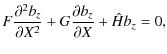
where

Here,
| (28) |
We seek a series solution to (24). First, hX(X,Y), hY(X,Y) and
|
(29) |
Similarly, F, G and
![\begin{figure}
\par\includegraphics[width=8.4cm,clip]{12669fg6.eps}
\end{figure}](/articles/aa/full_html/2010/03/aa12669-09/img133.png)
|
Figure 6:
Surface plots of energy density at
|
| Open with DEXTER | |
The next step is to choose a suitable form of series solution for bz. Led by the Frobenius solution to singular ordinary differential equations (ODEs), we put
Substituting all series expansions into (24) and equating powers of X provides the value of
Solving a second order ODE gives a 2-parameter solution which may be
written as a sum of two independent 1-parameter solutions. In such a
case the parameters are constants. The solution of the present partial
differential equation (PDE), which is second order in X, is analogous, making it possible to rewrite (30) as a sum of two 1-parameter solutions. Now, however, the parameters are functions of Y. Writing the solution for bz in this form gives
| bz | = | 
|
|
|
(31) |
where
|
(32) | ||
![$\displaystyle \hat{A}_{i,m}=-\frac{1}{m(m-2)F_1}\left[
\begin{array}{@{}c@{}}
-...
... G_{m-s}
\end{array}\right)\frac{\hat{B}_s\hat{H}_1}{2F_1}
\end{array}\right],$](/articles/aa/full_html/2010/03/aa12669-09/img158.png)
|
(33) |
with
This is a fully determined solution for bz. Series solutions for ![]() and
and ![]() follow naturally from
follow naturally from
| = | (34) | ||
| = | (35) |
Using a prime to denote differentiation with respect to Y, the leading order behaviour of the complete solution is
| bz | = | ||
| (36) | |||
| = | |||
| (37) | |||
| = | |||
| (38) |
where
|
(39) |
In the one dimensional limit, this solution reduces to the previously published solution for one dimensional resonant absorption.
The solution on the resonant contour can be examined by taking the limit
![]() ,
which gives
,
which gives
| bz | = | (40) | |
| = | (41) | ||
| = | (42) |
Thus,
![$\displaystyle u_Y=-i\left(\frac{B_0}{\mu_0\omega^2\left[\partial \rho/\partial ...
...0}}\right)\frac{1}{h_{Y0}}\left[\frac{{\rm d}b_z}{{\rm d}Y}\right]_{X=0}X^{-1}.$](/articles/aa/full_html/2010/03/aa12669-09/img179.png)
This is the velocity perturbation of the resonant Alfvén wave, which is the dominant feature for late times. Note the dependence on
6 Discussion and conclusions
We have established a mathematical basis by which resonant absorption may be understood when field line eigenfrequencies vary in two dimensions. This confirms that much of our intuitive understanding applies to these 2D equilibria. Particularly, energy is deposited as a phase mixing Alfvén wave where the field line eigenfrequency matches the driving frequency; a result that is also clear from Lee et al. (2000) and Terradas et al. (2008).
In both time-dependent simulations (after early times) and the analytic
solution, the system is dominated by a resonant Alfvén wave. The
velocity perturbation rapidly becomes parallel to the resonant surface,
so that
![]() .
Meanwhile,
.
Meanwhile,
![]() becomes much larger than
becomes much larger than
![]() .
In this limit, the governing equations tend to those for a decoupled
Alfvén wave. (See also the discussion of the ordering of perturbations
and length scales in Wright (1992).)
The dominant wave, which is localised about the surface at which the
local Alfvén speed matches the wave's field aligned phase speed, may
therefore be identified as an Alfvén wave.
.
In this limit, the governing equations tend to those for a decoupled
Alfvén wave. (See also the discussion of the ordering of perturbations
and length scales in Wright (1992).)
The dominant wave, which is localised about the surface at which the
local Alfvén speed matches the wave's field aligned phase speed, may
therefore be identified as an Alfvén wave.
The role of phase mixing in such a system may be followed using the phase mixing length, for which we have shown the generalisation from 1D to higher dimensions. This quantity is useful since it allows a simple estimate of the time required to develop small dissipative length scales. It therefore informs us which structures may be heated by resonant absorption within their typical lifetime, as well as providing a measure of the length scales to be considered for magnetospheric (and perhaps coronal) Alfvén waves.
The resonant Alfvén wave differs from the non-resonant, decoupled Alfvén wave in an important respect: it exhibits amplitude variations along contours of Alfvén frequency. These reveal the spatial form of the fast wave, the amplitude of the Alfvén wave correlating well with the magnetic pressure force of the fast wave. Intuitively, one can think of a resonant field line receiving a ``push'' from the fast wave during every period. These pushes are large where the amplitude of the magnetic pressure force is large, and small where the amplitude of the magnetic pressure force is small. After several cycles, those field lines which have received the largest pushes have the largest Alfvén oscillations. Alternatively, one can consider the variation of fast wave energy at the resonant surface. This is reflected in the energy available through resonance, leading to amplitude variations of the Alfvén wave.
In the magnetosphere, the correlation between the amplitude of the Alfvén wave and the amplitude of the magnetic pressure force offers a means of probing the magnetosphere through magnetoseismology. Observations of ULF magnetic pulsations over different magnetic latitudes and local times provide a spatial picture of the Alfvén wave, which, in turn, reveals the structure of the magnetospheric fast wave. This connection has already been exploited in weaker forms, for example, the low power of ULF waves at local noon and the dominance of antisunward azimuthal phase speeds led the community to consider antisunward propagating fast waves as the dominant driver (Samson et al. 1992; Anderson et al. 1990). More quantitatively, Wright & Rickard (1995) showed that a displacement pulse running along the magnetopause excites resonant Alfvén waves with an azimuthal phase velocity strictly equal to that of the boundary pulse. The present study suggests, however, that the correlation can be exploited more generally and invoking the amplitude also.
This work is readily applied to a coronal loop with a continuous profile of Alfvén speed. The kink frequency of a loop lies between the maximum Alfvén frequency within the loop and the Alfvén frequency of the environment, so the resonant contour exists for any continuous profile of field line eigenfrequencies. In this case, the total pressure perturbation associated with a transverse kink wave drives an Alfvén wave at the resonance, in the same manner as a fast wave.
For a cylindrical, monolithic loop, the total pressure perturbation of the kink wave has an ![]()
![]() symmetry where m=1.
We have seen that the amplitude of the magnetic pressure force
correlates with the amplitude of the resonant Alfvén wave, so the
resonant Alfvén wave will also have an m=1 symmetry (as in normal mode analysis).
It is therefore inevitable that the kink wave coexists with an m=1 Alfvén wave that oscillates at the kink frequency (Ruderman & Roberts 2002; Terradas et al. 2006).
symmetry where m=1.
We have seen that the amplitude of the magnetic pressure force
correlates with the amplitude of the resonant Alfvén wave, so the
resonant Alfvén wave will also have an m=1 symmetry (as in normal mode analysis).
It is therefore inevitable that the kink wave coexists with an m=1 Alfvén wave that oscillates at the kink frequency (Ruderman & Roberts 2002; Terradas et al. 2006).
Moving to more general equilibria, such as the elliptical cross-section considered by Ruderman (2003) or the multi-stranded loop of Terradas et al. (2008), resonant absorption continues to imprint the spatial form of the global mode of oscillation on the localised Alfvénic motions. This explains the complex variation of energy density on the resonant surface previously seen in Terradas et al. (2008) (their Fig. 10). The amplitude of global (kink-like) mode of oscillation must vary around this surface, with a form of magnetic pressure force captured in the energy density of the Alfvén wave.
In the analytic solution, magnetic pressure is not the only
contribution to amplitude variations of the resonant Alfvén wave.
Referring to Eq. (43), the Alfvénic velocity perturbation has a Y dependence of the form
![\begin{displaymath}\frac{1}{[\partial \rho/\partial X]_{X=0}}\frac{1}{h_{Y0}}\left[\frac{{\rm d}b_z}{{\rm d}Y}\right]_{X=0},\end{displaymath}](/articles/aa/full_html/2010/03/aa12669-09/img188.png)
noting that
Finally, it should now be possible to obtain a complete analytic solution for three dimensional resonant absorption with a straight, uniform magnetic field. Schulze-Berge et al. (1992) provide a framework, density variation along field lines may behandled by the methods of Thompson & Wright (1993) and the present paper contributes mathematical handling of two dimensional variation of field line eigenfrequencies.
AcknowledgementsA.J.B.R. is supported by an STFC studentship. We thank Jesse Andries and Fiona Russell for providing helpful comments during the preparation of this paper.
References
- Anderson, B. J., Engebretson, M. J., Rounds, S. P., Zanetti, L. J., & Potemra, T. A. 1990, J. Geophys. Res., 95, 10495 [NASA ADS] [CrossRef] [Google Scholar]
- Aschwanden, M. J. 2005, ApJ, 634, L193 [NASA ADS] [CrossRef] [Google Scholar]
- Aschwanden, M. J., & Nightingale, R. W. 2005, ApJ, 633, 499 [NASA ADS] [CrossRef] [Google Scholar]
- Aschwanden, M. J., Fletcher, L., Schrijver, C. J., & Alexander, D. 1999, ApJ, 520, 880 [NASA ADS] [CrossRef] [Google Scholar]
- Chen, L., & Hasegawa, A. 1974, Phys. Fluids, 17, 1399 [NASA ADS] [CrossRef] [Google Scholar]
- de Groof, A., Tirry, W. J., & Goossens, M. 1998, A&A, 335, 329 [NASA ADS] [Google Scholar]
- Dungey, J. W. 1955, in Physics of the Ionosphere, 229 [Google Scholar]
- Goossens, M., Hollweg, J. V., & Sakurai, T. 1992, Sol. Phys., 138, 233 [NASA ADS] [CrossRef] [Google Scholar]
- Hollweg, J. V., & Yang, G. 1988, J. Geophys. Res., 93, 5423 [NASA ADS] [CrossRef] [Google Scholar]
- Kivelson, M. G., & Southwood, D. J. 1985, Geophys. Res. Lett., 12, 49 [NASA ADS] [CrossRef] [Google Scholar]
- Lee, D.-H., Lysak, R. L., & Song, Y. 2000, J. Geophys. Res., 105, 10703 [NASA ADS] [CrossRef] [Google Scholar]
- Mann, I. R., & Wright, A. N. 1999, Geophys. Res. Lett., 26, 2609 [NASA ADS] [CrossRef] [Google Scholar]
- Mann, I. R., Wright, A. N., & Cally, P. S. 1995, J. Geophys. Res., 100, 19441 [NASA ADS] [CrossRef] [Google Scholar]
- Mann, I. R., Wright, A. N., Mills, K. J., & Nakariakov, V. M. 1999, J. Geophys. Res., 104, 333 [NASA ADS] [CrossRef] [Google Scholar]
- Martens, P. C. H., Cirtain, J. W., & Schmelz, J. T. 2002, ApJ, 577, L115 [NASA ADS] [CrossRef] [Google Scholar]
- Menk, F. W., Orr, D., Clilverd, M. A., et al. 1999, J. Geophys. Res., 104, 19955 [NASA ADS] [CrossRef] [Google Scholar]
- Nakariakov, V. M., Ofman, L., Deluca, E. E., Roberts, B., & Davila, J. M. 1999, Science, 285, 862 [NASA ADS] [CrossRef] [PubMed] [Google Scholar]
- Rezania, V., & Samson, J. C. 2005, A&A, 436, 999 [NASA ADS] [CrossRef] [EDP Sciences] [Google Scholar]
- Rickard, G. J., & Wright, A. N. 1994, J. Geophys. Res., 99, 13455 [NASA ADS] [CrossRef] [Google Scholar]
- Ruderman, M. S. 2003, A&A, 409, 287 [NASA ADS] [CrossRef] [EDP Sciences] [Google Scholar]
- Ruderman, M. S., & Roberts, B. 2002, ApJ, 577, 475 [NASA ADS] [CrossRef] [Google Scholar]
- Samson, J. C., Harrold, B. G., Ruohoniemi, J. M., Greenwald, R. A., & Walker, A. D. M. 1992, Geophys. Res. Lett., 19, 441 [NASA ADS] [CrossRef] [Google Scholar]
- Schmelz, J. T. 2002, ApJ, 578, L161 [NASA ADS] [CrossRef] [Google Scholar]
- Schmelz, J. T., Scopes, R. T., Cirtain, J. W., Winter, H. D., & Allen, J. D. 2001, ApJ, 556, 896 [NASA ADS] [CrossRef] [Google Scholar]
- Schmelz, J. T., Beene, J. E., Nasraoui, K., et al. 2003, ApJ, 599, 604 [NASA ADS] [CrossRef] [Google Scholar]
- Schmelz, J. T., Nasraoui, K., Richardson, V. L., et al. 2005, ApJ, 627, L81 [NASA ADS] [CrossRef] [Google Scholar]
- Schulze-Berge, S., Gowley, S., & Chen, L. 1992, J. Geophys. Res., 97, 3219 [NASA ADS] [CrossRef] [Google Scholar]
- Singer, H. J., Hughes, W. J., & Russell, C. T. 1982, J. Geophys. Res., 87, 3519 [NASA ADS] [CrossRef] [Google Scholar]
- Southwood, D. J. 1974, Planet. Space Sci., 22, 483 [NASA ADS] [CrossRef] [Google Scholar]
- Stewart, B. 1861, R. Soc. London Phil. Trans. Ser. I, 151, 423 [Google Scholar]
- Takahashi, K., & Anderson, B. J. 1992, J. Geophys. Res., 97, 10751 [NASA ADS] [CrossRef] [Google Scholar]
- Takahashi, K., Anderson, B. J., & Ohtani, S.-i. 1996, J. Geophys. Res., 101, 24815 [NASA ADS] [CrossRef] [Google Scholar]
- Terradas, J., Oliver, R., & Ballester, J. L. 2006, ApJ, 642, 533 [NASA ADS] [CrossRef] [Google Scholar]
- Terradas, J., Arregui, I., Oliver, R., et al. 2008, ApJ, 679, 1611 [NASA ADS] [CrossRef] [Google Scholar]
- Thompson, M. J., & Wright, A. N. 1993, J. Geophys. Res., 98, 15541 [NASA ADS] [CrossRef] [Google Scholar]
- Wright, A. N. 1992, J. Geophys. Res., 97, 6439 [NASA ADS] [CrossRef] [Google Scholar]
- Wright, A. N., & Rickard, G. J. 1995, J. Geophys. Res., 100, 23703 [NASA ADS] [CrossRef] [Google Scholar]
All Figures
|
|
Figure 1: Sketch of numerical domain showing boundary conditions. |
| Open with DEXTER | |
| In the text | |
|
|
Figure 2:
Cut in
|
| Open with DEXTER | |
| In the text | |
|
|
Figure 3:
Accumulation of energy density at a fully 2D resonant contour.
Plots show filled contours of energy density with contours representing |
| Open with DEXTER | |
| In the text | |
|
|
Figure 4: Phase mixing of velocity
component parallel to resonant contour. The plot is made along a curve
that is everywhere prependicular to contours of
|
| Open with DEXTER | |
| In the text | |
|
|
Figure 5:
Plots at
|
| Open with DEXTER | |
| In the text | |
|
|
Figure 6:
Surface plots of energy density at
|
| Open with DEXTER | |
| In the text | |
Copyright ESO 2010
Current usage metrics show cumulative count of Article Views (full-text article views including HTML views, PDF and ePub downloads, according to the available data) and Abstracts Views on Vision4Press platform.
Data correspond to usage on the plateform after 2015. The current usage metrics is available 48-96 hours after online publication and is updated daily on week days.
Initial download of the metrics may take a while.