| Issue |
A&A
Volume 510, February 2010
|
|
|---|---|---|
| Article Number | L6 | |
| Number of page(s) | 4 | |
| Section | Letters | |
| DOI | https://doi.org/10.1051/0004-6361/200913893 | |
| Published online | 18 February 2010 | |
LETTER TO THE EDITOR
Imprints of coronal temperature disturbances on type III bursts
B. Li - I. H. Cairns - P. A. Robinson
School of Physics, University of Sydney, New South Wales 2006, Australia
Received 17 December 2009 / Accepted 29 January 2010
Abstract
The electron temperature ![]() and ion temperature
and ion temperature ![]() in the corona vary with time and location, due to transient and
persistent activity on the Sun. The effects of spatially localized
disturbances in
in the corona vary with time and location, due to transient and
persistent activity on the Sun. The effects of spatially localized
disturbances in ![]() and
and ![]() on coronal type III radio bursts are simulated. The disturbances
are superimposed on monotonically varying temperature backgrounds
and arise from spatially confined solar activity, Qualitatively and
quantitatively different imprints are found on the curve of the maximum
flux versus frequency of type III bursts, because of the
disturbances in
on coronal type III radio bursts are simulated. The disturbances
are superimposed on monotonically varying temperature backgrounds
and arise from spatially confined solar activity, Qualitatively and
quantitatively different imprints are found on the curve of the maximum
flux versus frequency of type III bursts, because of the
disturbances in ![]() and
and ![]() .
The results indicate that nonthermal coronal type III bursts offer
a new tool to probe and distinguish between spatially localized
structures of
.
The results indicate that nonthermal coronal type III bursts offer
a new tool to probe and distinguish between spatially localized
structures of ![]() and
and ![]() along the paths of type III beams. Furthermore, localized
temperature disturbances may be responsible for some fine structures in
type III bursts, e.g., striae in type IIIb bursts in the
presence of multiple, localized temperature disturbances.
along the paths of type III beams. Furthermore, localized
temperature disturbances may be responsible for some fine structures in
type III bursts, e.g., striae in type IIIb bursts in the
presence of multiple, localized temperature disturbances.
Key words: Sun: radio radiation - Sun: corona - methods: numerical
1 Introduction
The solar corona is highly dynamic and activity occurs both impulsively
and continuously from small to large scales (e.g., microflares and
flares). The activity results in energy injection and heat transfer,
and so spatiotemporal variations in the temperature ![]() and density
and density ![]() of electrons, and the ion temperature
of electrons, and the ion temperature ![]() .
For instance, spatially confined activity such as X-ray bright
points may result in multiple, spatially localized disturbances in
.
For instance, spatially confined activity such as X-ray bright
points may result in multiple, spatially localized disturbances in ![]() and
and ![]() ,
as in Fig. 1.
These may remain distinct from each other because tangential
discontinuities can separate different thermal plasmas for long
periods. In addition,
,
as in Fig. 1.
These may remain distinct from each other because tangential
discontinuities can separate different thermal plasmas for long
periods. In addition, ![]() disturbances may be more localized and last much longer than
disturbances may be more localized and last much longer than ![]() disturbances,
because ions have much lower thermal speeds than electrons. Knowledge
of the spatial profiles of coronal temperatures is usually obtained by
using visible, UV, X-ray, and thermal radio emission.
This knowledge, currently inadequate, is vital to understanding
coronal heating and solar wind acceleration.
disturbances,
because ions have much lower thermal speeds than electrons. Knowledge
of the spatial profiles of coronal temperatures is usually obtained by
using visible, UV, X-ray, and thermal radio emission.
This knowledge, currently inadequate, is vital to understanding
coronal heating and solar wind acceleration.
![\begin{figure}
\par\includegraphics[width=7.5cm,clip]{13893fg1.eps}
\end{figure}](/articles/aa/full_html/2010/02/aa13893-09/img24.png)
|
Figure 1: Illustration of the production of localized regions with enhanced coronal temperatures in an open magnetic flux tube, through which a type III beam propagates (viewed from above the north pole). Localized regions R1-R3 are caused by three separate episodes of activity at localized solar source, with the latest activity producing R3. For clarity, the flux tube is assumed to have a regular spiral shape. |
| Open with DEXTER | |
Type III solar radio bursts are produced when energetic electrons
accelerated in flares propagate as beams along open magnetic field
lines into the interplanetary (IP) medium, and drive Langmuir (L) waves near the electron plasma frequency ![]() and radiation near
and radiation near ![]() and/or
and/or
![]() .
Coronal type IIIs are one of the most important diagnostics of
electron acceleration in flares and coronal conditions (Aschwanden 2002,2006).
For example, coronal type IIIs have been used to extract the
Sun's density profile, and solar-wind-like regions with
.
Coronal type IIIs are one of the most important diagnostics of
electron acceleration in flares and coronal conditions (Aschwanden 2002,2006).
For example, coronal type IIIs have been used to extract the
Sun's density profile, and solar-wind-like regions with
![]() are found to be common below
are found to be common below
![]() ,
where
,
where ![]() is the solar radius (Cairns et al. 2009).
is the solar radius (Cairns et al. 2009).
Sometimes, fine and/or sudden intensity changes in coronal type IIIs are observed (Fomichev & Chertok 1977; Suzuki & Dulk 1985). For example, type IIIb (stria) bursts show non-smooth variations in flux versus frequency, and chains of narrow-band structures are caused by successive modulations in flux (de La Noe & Boischot 1972). It has been variously conjectured that the flux modulations in type IIIb bursts occur because of modulational instability related to the dynamics of beam and L waves (Smith & de La Noe 1976), or filamentary coronal density structures (Takakura & Yousef 1975).
The primary aim of this letter is to demonstrate numerically the effects on coronal type IIIs
of spatially localized disturbances of ![]() and
and ![]() .
Our simulations show that
the dynamic spectrum of
.
Our simulations show that
the dynamic spectrum of
![]() emission is modulated at frequencies corresponding to the disturbances; so is the
emission is modulated at frequencies corresponding to the disturbances; so is the ![]() emission, although the predictions are generally below observable levels. Importantly, distinct imprints of the
emission, although the predictions are generally below observable levels. Importantly, distinct imprints of the ![]() and
and ![]() disturbances
exist on the curve of the maximum flux versus frequency for the
disturbances
exist on the curve of the maximum flux versus frequency for the
![]() emission.
The second aim is to show that detailed structures in coronal
type IIIs can be used to probe and ideally differentiate between
localized variations of
emission.
The second aim is to show that detailed structures in coronal
type IIIs can be used to probe and ideally differentiate between
localized variations of ![]() and
and ![]() along the beam path.
Fine structures resembling those in type IIIb bursts are produced
by multiple temperature disturbances, which suggests that localized
temperature disturbances may lead to type IIIb bursts.
along the beam path.
Fine structures resembling those in type IIIb bursts are produced
by multiple temperature disturbances, which suggests that localized
temperature disturbances may lead to type IIIb bursts.
2 Numerical model
The spatial variation in the ion temperature is defined by
![]() at time t=0, where x
is along the radial direction and represents the distance above the
photosphere. Since we assume that ions remain Maxwellian and unchanged
during the simulations, as in our earlier work (Li et al. 2008a,2008b),
at time t=0, where x
is along the radial direction and represents the distance above the
photosphere. Since we assume that ions remain Maxwellian and unchanged
during the simulations, as in our earlier work (Li et al. 2008a,2008b), ![]() retains
its original profile at all times. However, for an inhomogeneous plasma
with position-dependent electron temperature
retains
its original profile at all times. However, for an inhomogeneous plasma
with position-dependent electron temperature
![]() and/or density
and/or density
![]() ,
a source term needs to be added to the kinetic equation for electrons
to preserve the given
,
a source term needs to be added to the kinetic equation for electrons
to preserve the given
![]() and
and
![]() profiles
for simulation periods longer than the propagation time of a beam
traversing the simulation domain. The requirement to have a source term
arises because we allow electrons to evolve dynamically. Specifically,
the electron distribution function
profiles
for simulation periods longer than the propagation time of a beam
traversing the simulation domain. The requirement to have a source term
arises because we allow electrons to evolve dynamically. Specifically,
the electron distribution function
![]() evolves following (Li et al. 2002):
evolves following (Li et al. 2002):
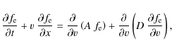
where v denotes electron speed. The first and second terms on the right-hand side (r.h.s.) of Eq. (1) represent spontaneous and induced emission, respectively, and the coefficient D describes the coupling between the beam and L waves. The density is given by
Under thermal and steady state conditions, ![]() is Maxwellian and given by
is Maxwellian and given by
![]() ,
where
,
where ![]() is the electron mass. The r.h.s. of Eq. (1) then vanishes because of the self-consistent definitions of A and D (Li et al. 2002). However, the left-hand side (l.h.s.) of Eq. (1) reduces to the advection term
is the electron mass. The r.h.s. of Eq. (1) then vanishes because of the self-consistent definitions of A and D (Li et al. 2002). However, the left-hand side (l.h.s.) of Eq. (1) reduces to the advection term
![]() ,
which is non-vanishing for plasmas with x-dependent
,
which is non-vanishing for plasmas with x-dependent ![]() and/or
and/or ![]() .
So a source term is required for Eq. (1) to remain self-consistent. We thus add a source term S(x,v) to the r.h.s. of Eq. (1), and set
.
So a source term is required for Eq. (1) to remain self-consistent. We thus add a source term S(x,v) to the r.h.s. of Eq. (1), and set

![$\displaystyle vf_\theta (n_{\rm e},T_{\rm e},v)\left[\frac{\partial}{\partial x...
...{v_{\rm e}^2}\!-\!1\right) \frac{\partial}{\partial x}\ln T_{\rm e}(x) \right],$](/articles/aa/full_html/2010/02/aa13893-09/img40.png)
where
We consider first the case in which the plasma has varying ![]() but uniform
but uniform ![]() ,
for which only the first term of Eq. (3) remains. For
,
for which only the first term of Eq. (3) remains. For
![]() monotonically increasing (decreasing) with increasing x, S>0 (S<0) for electrons with v>0, and so acts as a source (sink). In contrast, S is a sink (source) for electrons with v<0.
The physics of the case when
monotonically increasing (decreasing) with increasing x, S>0 (S<0) for electrons with v>0, and so acts as a source (sink). In contrast, S is a sink (source) for electrons with v<0.
The physics of the case when
![]() decreases monotonically is as follows. On the one hand, for v>0
more electrons move into rather than out of a given coronal layer
during a finite time interval. Thus, to maintain the given
decreases monotonically is as follows. On the one hand, for v>0
more electrons move into rather than out of a given coronal layer
during a finite time interval. Thus, to maintain the given ![]() and
and ![]() profiles a sink is needed to remove the excess electrons. On the other hand, for v<0
more electrons move out of than into the given layer,
so a source is required to supply the electrons lost because
of the imbalance.
profiles a sink is needed to remove the excess electrons. On the other hand, for v<0
more electrons move out of than into the given layer,
so a source is required to supply the electrons lost because
of the imbalance.
When ![]() is nonuniform but
is nonuniform but ![]() is homogeneous, only the second term of Eq. (3) remains. The nature (source or sink) of the S term now depends on both the trend of the
is homogeneous, only the second term of Eq. (3) remains. The nature (source or sink) of the S term now depends on both the trend of the ![]() profile and the electron speed, via the factors
profile and the electron speed, via the factors
![]() and
and
![]() ,
respectively. If we assume that
,
respectively. If we assume that ![]() monotonically increases with x, then at a given coronal layer statistically more electrons with
monotonically increases with x, then at a given coronal layer statistically more electrons with
![]() move outward rather than inward. To maintain the given
move outward rather than inward. To maintain the given ![]() and
and ![]() profiles, a source is therefore needed to supply the loss of electrons caused by the imbalance.
In contrast, at the same layer more slow electrons with
profiles, a source is therefore needed to supply the loss of electrons caused by the imbalance.
In contrast, at the same layer more slow electrons with
![]() move in rather than out, thus the excess electrons need to be drained away to retain the balance.
move in rather than out, thus the excess electrons need to be drained away to retain the balance.
In general, both terms in Eq. (3) remain for arbitrary, inhomogeneous profiles of ![]() and
and ![]() .
In the corona various effects may contribute to the source S.
For instance, small-scale activity, e.g., jets, can heat and
transport electrons between different locations, causing either gain or
loss of electrons at these locations.
.
In the corona various effects may contribute to the source S.
For instance, small-scale activity, e.g., jets, can heat and
transport electrons between different locations, causing either gain or
loss of electrons at these locations.
The simulations of coronal type IIIs use here our quasilinear-based model for plasma emission (Li et al. 2008a,2008b). The model includes a 3D source region with stratified 2D layers that vary with x, the dynamics of beam, L, ion-sound (S), and transverse waves coupled via quasilinear and nonlinear processes, and radiation propagation from the source to a remote observer. The model is generalized by including the term S in Eq. (1) which allows us to study the effects of localized temperature variations.
3 Simulation results
We assume that the coronal temperatures follow
![\begin{displaymath}%
T_s(x)=T_{\rm m}^s\left(1+\frac{x}{R_\odot}\right)^{-2/7} +...
...}\left[-\left(\frac{x-x_l^s}{\Delta x_l^s}\right)^{2} \right],
\end{displaymath}](/articles/aa/full_html/2010/02/aa13893-09/img46.png)
where
![\begin{figure}
\par\includegraphics[width=7.3cm,clip]{13893fg2.eps}
\end{figure}](/articles/aa/full_html/2010/02/aa13893-09/img54.png)
|
Figure 2:
Spatial profiles of |
| Open with DEXTER | |
Figure 2 shows the spatial profiles of ![]() and
and ![]() in the simulations.
Four different temperature conditions are considered: (
in the simulations.
Four different temperature conditions are considered: (
![]() )
both
)
both ![]() and
and ![]() decrease monotonically; (
decrease monotonically; (
![]() )
a localized
)
a localized ![]() disturbance is imposed on the background
disturbance is imposed on the background ![]() in
in
![]() ,
and
,
and ![]() is as in
is as in
![]() ;
(
;
(
![]() ) a localized
) a localized ![]() disturbance is imposed on the background
disturbance is imposed on the background ![]() in
in
![]() ,
and
,
and ![]() is as in
is as in
![]() ;
(
;
(
![]() ) three localized
) three localized ![]() disturbances are added to the background
disturbances are added to the background ![]() in
in
![]() ,
and
,
and ![]() is as in
is as in
![]() .
We assume that
.
We assume that
![]() MK for case
MK for case
![]() ,
which is much higher than the value of
,
which is much higher than the value of
![]() MK for cases
MK for cases
![]() and
and
![]() .
The Tls parametrization is based upon observations (e.g., Kohl et al. 1996), which show much higher coronal proton temperatures than
.
The Tls parametrization is based upon observations (e.g., Kohl et al. 1996), which show much higher coronal proton temperatures than ![]() ,
reaching 4-6 MK or higher at height
,
reaching 4-6 MK or higher at height
![]() .
Here we choose a higher
.
Here we choose a higher ![]() than observed so far to demonstrate clearly the effects of
than observed so far to demonstrate clearly the effects of ![]() localization.
localization.
We assume the 10-fold Baumbach-Allen model (Baumbach 1937; Allen 1947) for ![]() ,
and Fig. 2 also shows the resulting
,
and Fig. 2 also shows the resulting ![]() profile. The acceleration of electrons during flares is represented by adding a heating term H (Robinson & Benz 2000; Li et al. 2002) to the r.h.s. of Eq. (1):
profile. The acceleration of electrons during flares is represented by adding a heating term H (Robinson & Benz 2000; Li et al. 2002) to the r.h.s. of Eq. (1):
![]() .
Here a fraction
.
Here a fraction ![]() of electrons are heated from
of electrons are heated from ![]() to
to ![]() (
(
![]() )
over a typical region (
)
over a typical region (![]() ,
, ![]() )
centered at (
)
centered at (![]() ,
, ![]() ). Based on observations (Aschwanden 2002; Klein et al. 2005), we choose
). Based on observations (Aschwanden 2002; Klein et al. 2005), we choose
![]() ,
,
![]() MK,
MK,
![]() ms,
ms,
![]() ms,
ms,
![]() Gm, and
Gm, and
![]() Mm. Other simulation parameters are as in Li et al. (2008a).
Mm. Other simulation parameters are as in Li et al. (2008a).
Figures 3 and 4 show the dynamic spectrum of
![]() emission at Earth and the corresponding maximum flux
emission at Earth and the corresponding maximum flux
![]() versus frequency f, respectively, under the four different temperature conditions in Fig. 2. The
versus frequency f, respectively, under the four different temperature conditions in Fig. 2. The ![]() emission (not shown) is too weak, with flux
emission (not shown) is too weak, with flux ![]() solar flux unit (sfu) =
solar flux unit (sfu) =
![]() ,
to be observable
except for cases
,
to be observable
except for cases
![]() and
and
![]() .
This is due primarily to strong free-free absorption, strong
radiation loss by scattering, and weak source emission (Robinson &
Benz 2000; Li et al. 2008a). Below we discuss mainly the
.
This is due primarily to strong free-free absorption, strong
radiation loss by scattering, and weak source emission (Robinson &
Benz 2000; Li et al. 2008a). Below we discuss mainly the
![]() results.
results.
![\begin{figure}
\par\includegraphics[width=7.3cm,clip]{13893fg3.eps}
\end{figure}](/articles/aa/full_html/2010/02/aa13893-09/img73.png)
|
Figure 3:
Simulated
|
| Open with DEXTER | |
![\begin{figure}
\par\includegraphics[width=7.2cm,clip]{13893fg4.eps}\vspace*{-2mm}
%
\end{figure}](/articles/aa/full_html/2010/02/aa13893-09/img74.png)
|
Figure 4:
Maximum
|
| Open with DEXTER | |
First, Figs. 3a and 4 (black curve) show that for case
![]() the spectrum varies smoothly, and
the spectrum varies smoothly, and
![]() decreases with f
after radiation onset, respectively. These properties and other
spectral characteristics, e.g., drift rate (not shown), agree
quantitatively with typical observations, as in our previous work
(Li et al. 2008a).
decreases with f
after radiation onset, respectively. These properties and other
spectral characteristics, e.g., drift rate (not shown), agree
quantitatively with typical observations, as in our previous work
(Li et al. 2008a).
Figure 3b shows the
![]() spectrum for case
spectrum for case
![]() .
The spectrum is modulated
at f corresponding to the
.
The spectrum is modulated
at f corresponding to the ![]() disturbance, and the flux is suppressed close to the center of the disturbance. Figure 4 (green curve) illustrates fine structures in
disturbance, and the flux is suppressed close to the center of the disturbance. Figure 4 (green curve) illustrates fine structures in
![]() caused by the disturbance. Specifically, as f varies from high to low frequencies
caused by the disturbance. Specifically, as f varies from high to low frequencies
![]() varies according to the sequence ``same
varies according to the sequence ``same
![]() decrease
decrease
![]() increase
increase
![]() same'', relative to case
same'', relative to case
![]() .
In addition,
.
In addition,
![]() is modulated within the range
is modulated within the range
![]() MHz, corresponding to the disturbed region between
MHz, corresponding to the disturbed region between
![]() and
and
![]() .
Furthermore,
.
Furthermore,
![]() reaches a local minimum and maximum at
reaches a local minimum and maximum at
![]() MHz
MHz ![]()
![]() MHz and
MHz and
![]() MHz, decreasing and increasing by factors of
MHz, decreasing and increasing by factors of
![]() and
and
![]() relative to case
relative to case
![]() ,
respectively.
,
respectively.
Physically, on entering the region with increasing ![]() ,
the beam becomes relatively narrower and slightly faster because
,
the beam becomes relatively narrower and slightly faster because ![]() extends to higher v. This causes the weaker growth of L waves, mainly because less free energy is available, although the collisional damping rate (
extends to higher v. This causes the weaker growth of L waves, mainly because less free energy is available, although the collisional damping rate (
![]() )
of L waves decreases slightly (Li et al. 2008b). The source
)
of L waves decreases slightly (Li et al. 2008b). The source
![]() emission
is thus weaker, so is the remote radiation, although loss by
free-free absorption is reduced locally because
emission
is thus weaker, so is the remote radiation, although loss by
free-free absorption is reduced locally because ![]() increases. On passing the central region of the disturbance, the beam becomes relatively wider and slower because
increases. On passing the central region of the disturbance, the beam becomes relatively wider and slower because ![]() decreases.
The combined effects of more free energy now being available and the lower collisional damping rate result in stronger L waves, and so stronger source
decreases.
The combined effects of more free energy now being available and the lower collisional damping rate result in stronger L waves, and so stronger source
![]() emission.
Remote radiation is further strongly enhanced because of the locally
weaker free-free absorption. On exiting the disturbed region,
the beam, source waves, and radiation recover their properties for
case
emission.
Remote radiation is further strongly enhanced because of the locally
weaker free-free absorption. On exiting the disturbed region,
the beam, source waves, and radiation recover their properties for
case
![]() .
.
Figure 3c shows the
![]() spectrum for case
spectrum for case
![]() with a single localized
with a single localized ![]() disturbance. The spectrum appears qualitatively similar to that in Fig. 3b in terms of spectral modulation. However, detailed examination of the variation in
disturbance. The spectrum appears qualitatively similar to that in Fig. 3b in terms of spectral modulation. However, detailed examination of the variation in
![]() versus f in Fig. 4 (red curve) shows both qualitative and quantitative differences and similarities exist relative to case
versus f in Fig. 4 (red curve) shows both qualitative and quantitative differences and similarities exist relative to case
![]() ,
as follows:
,
as follows:
- 1.
- The sequence of
 versus f from high to low frequencies relative to case
 is ``same
 increase
decrease
increase
same'', which is distinct from that for case
increase
decrease
increase
same'', which is distinct from that for case
 .
.
- 2.
- The frequencies
 MHz and 154 MHz of the two local peaks, and
 MHz
at the center of the local dip differ evidently from, and is
quantitatively similar to, those of the single peak and trough for
case
,
respectively.
MHz
at the center of the local dip differ evidently from, and is
quantitatively similar to, those of the single peak and trough for
case
,
respectively.
- 3.
- The quantitative modulation effects on
caused by the
 disturbance are weaker than those caused by the
  disturbance. For instance,
increases by a factor
disturbance. For instance,
increases by a factor
 at the two local peaks relative to case
.
This factor is smaller than the factor
at the two local peaks relative to case
.
This factor is smaller than the factor
 for case
,
where
increases locally by
for case
,
where
increases locally by  ,
while
here increases locally by a factor
,
while
here increases locally by a factor  .
.
- 4.
- The frequency region of the
modulation is basically the same as for case
.
The trend of
![]() versus f for case
versus f for case
![]() in Fig. 4 is caused by the following. As the beam enters the region where
in Fig. 4 is caused by the following. As the beam enters the region where ![]() increases, the product L waves become stronger because of the stronger ES decay, leading to stronger
increases, the product L waves become stronger because of the stronger ES decay, leading to stronger
![]() source emission (produced by coupling between primary and product L waves), hence stronger remote emission (Li et al. 2005). However, as
source emission (produced by coupling between primary and product L waves), hence stronger remote emission (Li et al. 2005). However, as ![]() increases further, the level of primary L waves decreases because the even stronger decay process transfer the primary L wave energy into the product L waves (Li et al. 2003). The forward-directed (anti-Sunward) emission is thus weaker. Consequently, a local dip in
increases further, the level of primary L waves decreases because the even stronger decay process transfer the primary L wave energy into the product L waves (Li et al. 2003). The forward-directed (anti-Sunward) emission is thus weaker. Consequently, a local dip in
![]() appears at frequencies corresponding to where
appears at frequencies corresponding to where ![]() maximizes. In the simulations, we neglected the backward-directed
maximizes. In the simulations, we neglected the backward-directed
![]() emission, which is generated by coupling between product L waves (Li et al. 2008a). In general, the backward emission contributes negligibly to
emission, which is generated by coupling between product L waves (Li et al. 2008a). In general, the backward emission contributes negligibly to
![]() because
the radiation is partly lost and time-delayed by strong scattering and
reflection closer to the Sun and undergoes additional free-free
absorption before reaching the observer, although it may affect the
temporal profile of the
because
the radiation is partly lost and time-delayed by strong scattering and
reflection closer to the Sun and undergoes additional free-free
absorption before reaching the observer, although it may affect the
temporal profile of the
![]() flux (Riddle 1974). As the beam propagates further,
flux (Riddle 1974). As the beam propagates further, ![]() decreases, leading to relatively stronger coupling between the primary and product L waves,
and thus stronger forward
decreases, leading to relatively stronger coupling between the primary and product L waves,
and thus stronger forward
![]() emission and higher values of
emission and higher values of
![]() .
Once the beam passes the disturbed region, the source waves and remote radiation regain the properties for case
.
Once the beam passes the disturbed region, the source waves and remote radiation regain the properties for case
![]() .
.
We also found (not shown) for case
![]() that the flux of
that the flux of ![]() emission is significantly enhanced (
emission is significantly enhanced (![]() sfu) above the thermal level and may be observable as a microburst (Kundu et al. 1986) at frequencies corresponding to the disturbance. This occurs mainly because the S waves are stronger and the
sfu) above the thermal level and may be observable as a microburst (Kundu et al. 1986) at frequencies corresponding to the disturbance. This occurs mainly because the S waves are stronger and the ![]() emission rate is higher for higher
emission rate is higher for higher ![]() .
.
Finally, Figs. 3d and 4 (blue curve) show the
![]() spectrum and
spectrum and
![]() versus f, respectively, for case
versus f, respectively, for case
![]() .
We see that the spectrum is repeatedly modulated, each modulation resembling that in Fig. 3b. Furthermore, the variations in
.
We see that the spectrum is repeatedly modulated, each modulation resembling that in Fig. 3b. Furthermore, the variations in
![]() versus f clearly show the same signature for each
versus f clearly show the same signature for each ![]() disturbance
as found for case
disturbance
as found for case
![]() .
Thus, the signature of
.
Thus, the signature of
![]() variations with f for a single
variations with f for a single ![]() disturbance is robust. Figure 4 also shows that greater disturbances in
disturbance is robust. Figure 4 also shows that greater disturbances in ![]() relative to the background lead to qualitatively greater modulations in
relative to the background lead to qualitatively greater modulations in
![]() (cf., the peak
(cf., the peak
![]() values for the first and third
values for the first and third ![]() disturbances). Similar results are found for multiple
disturbances). Similar results are found for multiple ![]() disturbances (not shown).
disturbances (not shown).
4 Discussion and conclusions
We have developed the first simulations to study the effects on coronal
type IIIs of spatially localized disturbances in ![]() or
or ![]() .
The disturbances may be produced by various coronal activities, so the simulations are more realistic than previous work.
.
The disturbances may be produced by various coronal activities, so the simulations are more realistic than previous work.
The simulations demonstrate that the dynamic spectrum and the curve of maximum flux
![]() versus frequency f for
versus frequency f for
![]() emission are modulated by the
emission are modulated by the ![]() or
or ![]() disturbances. Crucially, the modulation fine structures differ for
disturbances. Crucially, the modulation fine structures differ for ![]() and
and ![]() disturbances, both qualitatively and quantitatively. A localized increase in
disturbances, both qualitatively and quantitatively. A localized increase in ![]() produces a signature of ``trough
produces a signature of ``trough
![]() peak'' in the
peak'' in the
![]() versus f curve, while a ``peak
versus f curve, while a ``peak
![]() trough
trough
![]() peak'' signature occurs for a localized increase in
peak'' signature occurs for a localized increase in ![]() .
The different signatures are robust and independent of the details of the disturbances. Thus, localized
.
The different signatures are robust and independent of the details of the disturbances. Thus, localized ![]() and
and ![]() disturbances leave identifiable imprints on
disturbances leave identifiable imprints on
![]() emission. In addition, weak
emission. In addition, weak ![]() emission may be observable for sufficiently large
emission may be observable for sufficiently large ![]() disturbances.
One implication is that the detailed frequency fine structures in
coronal type IIIs can be used to probe and differentiate between
the localized profiles of
disturbances.
One implication is that the detailed frequency fine structures in
coronal type IIIs can be used to probe and differentiate between
the localized profiles of ![]() and
and ![]() .
Thus nonthermal coronal type IIIs offer a new tool to remotely diagnose
spatial temperature structures in the corona.
.
Thus nonthermal coronal type IIIs offer a new tool to remotely diagnose
spatial temperature structures in the corona.
We also found that larger disturbances in ![]() or
or ![]() relative to the background results in qualitatively larger amplitude modulations in
relative to the background results in qualitatively larger amplitude modulations in
![]() .
Furthermore, for the same disturbance in temperature the modulation effects on
.
Furthermore, for the same disturbance in temperature the modulation effects on
![]() are more pronounced for
are more pronounced for ![]() than for
than for ![]() ,
as suggested by Fig. 4.
,
as suggested by Fig. 4.
The modulations in
![]() spectrum caused by multiple
spectrum caused by multiple ![]() or
or ![]() disturbances
resemble qualitatively the fine structures in
type IIIb bursts. Thus, our results suggest that localized
disturbances in
disturbances
resemble qualitatively the fine structures in
type IIIb bursts. Thus, our results suggest that localized
disturbances in ![]() or
or ![]() may produce type IIIs with striae and modulations in f. This mechanism differs from those previously proposed, e.g., modulational instability (Smith & de La Noe 1976) or filamentary density structures (Takakura & Yousef 1975).
may produce type IIIs with striae and modulations in f. This mechanism differs from those previously proposed, e.g., modulational instability (Smith & de La Noe 1976) or filamentary density structures (Takakura & Yousef 1975).
The flux modulation mechanism here may also apply to type III beams that cross shocks. MacDowall (1989)
observed that the flux of IP type IIIs changed suddenly as
beams neared shocks. He suggested that the changes are caused by
the scattering of beam electrons by magnetic turbulence. We propose,
instead, that the heating of electrons and ions just downstream of the
shocks produces localized increases in ![]() and
and ![]() ,
and so modulations in flux.
,
and so modulations in flux.
The Australian Research Council supported this work.
References
- Allen, C. W. 1947, MNRAS, 107, 426 [NASA ADS] [Google Scholar]
- Aschwanden, M. J. 2002, Space Sci. Rev., 101, 1 [NASA ADS] [CrossRef] [Google Scholar]
- Aschwanden, M. J. 2006, Physics of the Solar Corona: An Introduction with Problems and Solutions (Springer, Berlin), Chapter 15 [Google Scholar]
- Baumbach, S. 1937, Astron. Nachr., 263, 131 [Google Scholar]
- Cairns, I. H., Lobzin, V. V., Warmuth, A., et al. 2009, ApJ, 706, L265 [NASA ADS] [CrossRef] [Google Scholar]
- de La Noe, J., & Boischot, A. 1972, A&A, 20, 55 [NASA ADS] [Google Scholar]
- Fomichev, V. V., & Chertok, I. M. 1977, Radiophys. Quantum Electron., 20, 869 [NASA ADS] [CrossRef] [Google Scholar]
- Klein, K.-L., Krucker, S., Trottet, G., & Hoang, S. 2005, A&A, 431, 1047 [NASA ADS] [CrossRef] [EDP Sciences] [Google Scholar]
- Kohl, J. L., Strachan, L., & Gardner, L. D. 1996, ApJ, 465, L141 [NASA ADS] [CrossRef] [Google Scholar]
- Kundu, M. R., Gergely, T. E., Szabo, A., Loiacono, R., & White, S. M. 1986, ApJ, 308, 436 [NASA ADS] [CrossRef] [Google Scholar]
- Li, B., Robinson, P. A., & Cairns, I. H. 2002, Phys. Plasmas, 9, 2976 [NASA ADS] [CrossRef] [Google Scholar]
- Li, B., Willes, A. J., Robinson, P. A., & Cairns, I. H. 2003, Phys. Plasmas, 10, 2748 [NASA ADS] [CrossRef] [Google Scholar]
- Li, B., Willes, A. J., Robinson, P. A., & Cairns, I. H. 2005, Phys. Plasmas, 12, 012103; 052324 [NASA ADS] [CrossRef] [Google Scholar]
- Li, B., Cairns, I. H., & Robinson, P. A. 2008a, J. Geophys. Res., 113, A06104, A06105 [Google Scholar]
- Li, B., Robinson, P. A., & Cairns, I. H. 2008b, J. Geophys. Res., A10101 [Google Scholar]
- MacDowall, R. J. 1989, Geophys. Res. Lett., 16, 923 [NASA ADS] [CrossRef] [Google Scholar]
- Parker, E. N. 2007, in Handbook of the Solar-Terrestrial Environment, ed. Y. Kamide, & A. Chian (Springer, Berlin), 95 [Google Scholar]
- Riddle, A. C. 1974, Sol. Phys., 35, 153 [NASA ADS] [CrossRef] [Google Scholar]
- Robinson, P. A., & Benz, A. O. 2000, Sol. Phys., 194, 345 [Google Scholar]
- Smith, R. A., & de La Noe, J. 1976, ApJ, 207, 605 [NASA ADS] [CrossRef] [Google Scholar]
- Suzuki, S., & Dulk, G. A. 1985, in Solar Radiophysics, ed. D. J. McLean, & N. R. Labrum (Cambridge: Cambridge Univ. Press), 289 [Google Scholar]
- Takakura, T., & Yousef, S. 1975, Sol. Phys., 40, 421 [NASA ADS] [CrossRef] [Google Scholar]
All Figures
|
|
Figure 1: Illustration of the production of localized regions with enhanced coronal temperatures in an open magnetic flux tube, through which a type III beam propagates (viewed from above the north pole). Localized regions R1-R3 are caused by three separate episodes of activity at localized solar source, with the latest activity producing R3. For clarity, the flux tube is assumed to have a regular spiral shape. |
| Open with DEXTER | |
| In the text | |
|
|
Figure 2:
Spatial profiles of |
| Open with DEXTER | |
| In the text | |
|
|
Figure 3:
Simulated
|
| Open with DEXTER | |
| In the text | |
|
|
Figure 4:
Maximum
|
| Open with DEXTER | |
| In the text | |
Copyright ESO 2010
Current usage metrics show cumulative count of Article Views (full-text article views including HTML views, PDF and ePub downloads, according to the available data) and Abstracts Views on Vision4Press platform.
Data correspond to usage on the plateform after 2015. The current usage metrics is available 48-96 hours after online publication and is updated daily on week days.
Initial download of the metrics may take a while.