| Issue |
A&A
Volume 510, February 2010
|
|
|---|---|---|
| Article Number | A107 | |
| Number of page(s) | 9 | |
| Section | Planets and planetary systems | |
| DOI | https://doi.org/10.1051/0004-6361/200912910 | |
| Published online | 18 February 2010 | |
Multi-band transit observations of the TrES-2b exoplanet![[*]](/icons/foot_motif.png)
D. Mislis1 - S. Schröter1 - J. H. M. M. Schmitt1 - O. Cordes2 - K. Reif2
1 - Hamburger Sternwarte, Gojenbergsweg 112, 21029 Hamburg, Germany
2 -
Argelander-Institut für Astronomie, Auf dem Hügel 71, 53121 Bonn, Germany
Received 17 July 2009 / Accepted 14 December 2009
Abstract
We present a new data set of transit observations of the TrES-2b
exoplanet taken in spring 2009, using the 1.2 m Oskar-Lühning
telescope (OLT) of Hamburg Observatory and the 2.2 m telescope at
Calar Alto Observatory using BUSCA (Bonn University Simultaneous
CAmera). Both the new OLT data, taken with the same instrumental setup
as our data taken in 2008, as well as the simultaneously recorded
multicolor BUSCA data confirm the low inclination values reported
previously, and in fact suggest that the TrES-2b exoplanet has already
passed the first inclination threshold
![]() and is not eclipsing the full stellar surface any longer. Using the
multi-band BUSCA data we demonstrate that the multicolor light curves
can be consistently fitted with a given set of limb darkening
coefficients without the need to adjust these coefficients, and
further, we can demonstrate that wavelength dependent stellar radius
changes must be small as expected from theory. Our new observations
provide further evidence for a change of the orbit inclination of the
transiting extrasolar planet TrES-2b reported previously. We examine in
detail possible causes for this inclination change and argue that the
observed change should be interpreted as nodal regression. While the
assumption of an oblate host star requires an unreasonably large second
harmonic coefficient, the existence of a third body in the form of an
additional planet would provide a very natural explanation for the
observed secular orbit change. Given the lack of clearly observed
short-term variations of transit timing and our observed secular nodal
regression rate, we predict a period between approximately 50 and 100
days for a putative perturbing planet of Jovian mass. Such an object
should be detectable with present-day radial velocity (RV) techniques,
but would escape detection through transit timing variations.
and is not eclipsing the full stellar surface any longer. Using the
multi-band BUSCA data we demonstrate that the multicolor light curves
can be consistently fitted with a given set of limb darkening
coefficients without the need to adjust these coefficients, and
further, we can demonstrate that wavelength dependent stellar radius
changes must be small as expected from theory. Our new observations
provide further evidence for a change of the orbit inclination of the
transiting extrasolar planet TrES-2b reported previously. We examine in
detail possible causes for this inclination change and argue that the
observed change should be interpreted as nodal regression. While the
assumption of an oblate host star requires an unreasonably large second
harmonic coefficient, the existence of a third body in the form of an
additional planet would provide a very natural explanation for the
observed secular orbit change. Given the lack of clearly observed
short-term variations of transit timing and our observed secular nodal
regression rate, we predict a period between approximately 50 and 100
days for a putative perturbing planet of Jovian mass. Such an object
should be detectable with present-day radial velocity (RV) techniques,
but would escape detection through transit timing variations.
Key words: planetary systems - techniques: photometric - stars: individual: TrES-2b
1 Introduction
As of now more than 400 extrasolar planets have been detected around solar-like stars. In quite a few cases several planets have been detected to orbit a given star, demonstrating the existence of extrasolar planet systems in analogy to our solar system. Just as the planets in our solar system interact gravitationally, the same must apply to extrasolar planet systems. Gravitational interactions are important for the understanding of the long-term dynamical stability of planetary systems. The solar system has been around for more than four billion years, and the understanding of its dynamical stability over that period of time is still a challenge Simon et al. (1994). In analogy, extrasolar planet systems must be dynamically stable over similarly long time scales, and most stability studies of extrasolar planet systems have been directed towards an understanding of exactly those long time scales. Less attention has been paid to secular and short-term perturbations of the orbit, since such effects are quite difficult to detect observationally. Miralda-Escudé (2002) gives a detailed discussion on what secular effects might be derivable from extrasolar planet transits; in spectroscopic binaries the orbit inclination i can only be deduced in conjunction with the companion mass, and therefore the detection of an orbit inclination change is virtually impossible. Short-term transit timing variations (TTVs) have been studied by a number of authors (Agol et al. 2005; Holman & Murray 2005), however, a detection of such effects has remained elusive so far. In principle, a detection of orbit change would be extremely interesting since it would open up entirely new diagnostic possibilities of the masses and orbit geometries of these systems; also, in analogy to the discovery of Neptune, new planets could in fact be indirectly detected.
The lightcurve of a transiting extrasolar planet with known period
allows very accurate determinations
of the radii of star and planet (relative to the semi-major axis) and
the inclination
of the orbital plane of the planet with respect to the line of sight
towards the observer. Clearly, one does not expect the sizes of host
star and planet to vary on short time scales, however, the presence of
a third body can change the orientation of the orbit plane and, hence,
lead to a change in the observed inclination with respect to the
celestial plane. The TrES-2 exoplanet is particularly interesting in
this context. It orbits
its host star once in 2.47 days, which itself is very much
solar-like with parameters consistent with solar parameters; its age is
considerable and, correspondingly, the star rotates quite slowly. Its
close-in planet with a size of 1.2
![]() is among the most massive known transiting extrasolar planets (Holman et al. 2007; Sozzetti et al. 2007).
is among the most massive known transiting extrasolar planets (Holman et al. 2007; Sozzetti et al. 2007).
What makes the TrES-2 exoplanet orbits even more interesting, is
the fact that an apparent inclination change has been reported by some
of us in a previous paper (Mislis & Schmitt 2009,
henceforth called Paper I). The authors carefully measured several
transits observed in 2006 and 2008. Assuming a circular orbit with
constant period P, the duration of an extrasolar planet transit in
front of its host star depends only on the stellar and planetary radii, ![]() and
and ![]() ,
and on the inclination i of the orbit plane w.r.t. the sky plane. A linear best fit to the currently
available inclination measurements yields an apparent inclination decrease of
,
and on the inclination i of the orbit plane w.r.t. the sky plane. A linear best fit to the currently
available inclination measurements yields an apparent inclination decrease of
![]() deg/day. The transit modeling both by Holman et al. (2007) and Mislis & Schmitt (2009)
shows the transit of TrES-2b in front of its host star to be
``grazing''. In fact, according to the latest modeling the planet
occults only a portion of the host star and transits are expected to
disappear in the time frame 2020-2025, if the observed linear trend
continues. This ``grazing'' viewing geometry is particularly suitable
for the detection of orbital changes, since relatively small changes in
apparent inclination translate into relatively large changes in eclipse
duration. At the same time, a search for possible TTVs
by Rabus et al. (2009) has been negative; while Rabus et al. (2009) derive a period wobble of 57 s for TrES-2, the statistical quality of
their data is such that no unique periods for TTVs can be identified.
deg/day. The transit modeling both by Holman et al. (2007) and Mislis & Schmitt (2009)
shows the transit of TrES-2b in front of its host star to be
``grazing''. In fact, according to the latest modeling the planet
occults only a portion of the host star and transits are expected to
disappear in the time frame 2020-2025, if the observed linear trend
continues. This ``grazing'' viewing geometry is particularly suitable
for the detection of orbital changes, since relatively small changes in
apparent inclination translate into relatively large changes in eclipse
duration. At the same time, a search for possible TTVs
by Rabus et al. (2009) has been negative; while Rabus et al. (2009) derive a period wobble of 57 s for TrES-2, the statistical quality of
their data is such that no unique periods for TTVs can be identified.
The purpose of this paper is to present new transit observations of the TrES-2 exoplanet system obtained in 2009, which are described in the first part (Sect. 2) and analysed (Sect. 3). In the second part (Sect. 4) of our paper we present a quantitatively analysis of what kind of gravitational effects can be responsible for the observed orbit changes of TrES-2b and are consistent with all observational data of the TrES-2 system.
2 Observations and data reduction
We observed two transits of TrES-2 using the ephemeris suggested by O'Donovan et al. (2006) and by Holman et al. (2007) from
![]() ,
using the 1.2 m Oskar Lühning telescope (OLT) at Hamburg
Observatory and Calar Alto Observatory 2.2 m telescope with BUSCA.
,
using the 1.2 m Oskar Lühning telescope (OLT) at Hamburg
Observatory and Calar Alto Observatory 2.2 m telescope with BUSCA.
The OLT data were taken on 11 April 2009 using a
![]() CCD with a
CCD with a
![]() FOV and an I-band filter as in our previous observing run (Paper I). The readout noise and the gain were
16.37 e- and 1.33 e-/ADU
respectively. With the OLT we used 60-s exposures which provided an
effective time resolution of 1.17 min. During the observation, the
airmass value ranged from 1.7877 to 1.0712 and the seeing was typically
2.94''.
FOV and an I-band filter as in our previous observing run (Paper I). The readout noise and the gain were
16.37 e- and 1.33 e-/ADU
respectively. With the OLT we used 60-s exposures which provided an
effective time resolution of 1.17 min. During the observation, the
airmass value ranged from 1.7877 to 1.0712 and the seeing was typically
2.94''.
The Calar Alto data were taken on 28 May 2009 using BUSCA and
the 2.2 m telescope. BUSCA is designed to perform simultaneous
observations in four individual bands with a FOV of
![]() .
Therefore it has four individual
.
Therefore it has four individual
![]() CCD systems which cover the ultra-violet, the blue-green, the
yellow-red and the near-infrared part of the spectrum (channel a-d
respectively). For this run we used the Strömgren filters v (chn. a), b
(chn. b), and y (chn. c), and a Cousins-I filter for the near-infrared (chn. d). The readout-noise for these four detectors are
9.09 e-, 3.50 e-, 3.72 e-, and 3.86 e- respectively for the a, b, c, and d channels. The gain values for the same channels are 1.347 e-/ADU, 1.761 e-/ADU, 1.733 e-/ADU, and 1.731 e-/ADU respectively. The airmass value ranged from 1.8827 to 1.0453 and the seeing was 3.09''. For the BUSCA observations we
took 30 s exposure yielding an effective time resolution of 1.63 min. In Table 1 we summarize the relevant observation details.
CCD systems which cover the ultra-violet, the blue-green, the
yellow-red and the near-infrared part of the spectrum (channel a-d
respectively). For this run we used the Strömgren filters v (chn. a), b
(chn. b), and y (chn. c), and a Cousins-I filter for the near-infrared (chn. d). The readout-noise for these four detectors are
9.09 e-, 3.50 e-, 3.72 e-, and 3.86 e- respectively for the a, b, c, and d channels. The gain values for the same channels are 1.347 e-/ADU, 1.761 e-/ADU, 1.733 e-/ADU, and 1.731 e-/ADU respectively. The airmass value ranged from 1.8827 to 1.0453 and the seeing was 3.09''. For the BUSCA observations we
took 30 s exposure yielding an effective time resolution of 1.63 min. In Table 1 we summarize the relevant observation details.
Table 1: Observation summary.
For the data reduction, we used Starlink and DaoPhot software routines, and the MATCH
code. We perform the normal reduction tasks, bias subtraction, dark
correction, and flat fielding on the individual data sets before
applying aperture photometry on on all images. For TrES-2, we selected
the aperture photometry mode using apertures centered on the target
star, check stars, and sky background. Typical sky brightness values
for the 11 April and for the 28 May were 89 and 98 ADUs, respectively,
i.e., values at a level ![]() and
and ![]() of the star's flux,
respectively (for I-filter).
For the relative photometry we used the star U1350-10220179 as a
reference star to test and calibrate the light curve. For the data
analysis presented in this paper we did not use additional check stars,
but note that we already checked this star for constancy in the
Paper I. To estimate the magnitude errors, we followed Howell & Everett (2001) and
the same procedure as described in our first paper (Paper I) to
obtain better relative results. Our final relative photometry is
presented in Table 2, which is
available in its entirety in machine-readable form in the electronic version of this paper.
of the star's flux,
respectively (for I-filter).
For the relative photometry we used the star U1350-10220179 as a
reference star to test and calibrate the light curve. For the data
analysis presented in this paper we did not use additional check stars,
but note that we already checked this star for constancy in the
Paper I. To estimate the magnitude errors, we followed Howell & Everett (2001) and
the same procedure as described in our first paper (Paper I) to
obtain better relative results. Our final relative photometry is
presented in Table 2, which is
available in its entirety in machine-readable form in the electronic version of this paper.
Table 2: Relative photometry data.
3 Model analysis and results
In our model analysis we proceeded in exactly the same fashion as
described in Paper I. Note that the assumption of circularity
appears to apply very well to
TrES-2b (O'Donovan et al. 2009; O'Donovan et al. 2006); the assumption of constant period and hence constant semi-major axis will be adressed in
Sect. 4. For our modelling
we specifically assumed the values
![]() ,
,
![]() ,
P=2.470621 days,
,
P=2.470621 days,
![]() AU for the radii of star and planet, their period and the orbit radius
respectively. All limb darkening coefficients were taken from Claret (2004), and for the OLT data we used the same values as in Paper I, viz., u1 = 0.318 and u2 = 0.295 for the I filter, as denoted by S1 in Table 3.
AU for the radii of star and planet, their period and the orbit radius
respectively. All limb darkening coefficients were taken from Claret (2004), and for the OLT data we used the same values as in Paper I, viz., u1 = 0.318 and u2 = 0.295 for the I filter, as denoted by S1 in Table 3.
3.1 OLT data and modeling
Table 3:
Individual values of duration, inclination, ![]() values and limb darkening coefficients from five light curve fits.
values and limb darkening coefficients from five light curve fits.
![\begin{figure}
\par\includegraphics[width=9cm,clip]{Fig001.eps}
\end{figure}](/articles/aa/full_html/2010/02/aa12910-09/img27.png)
|
Figure 1: Observed TrES-2 light curves and model fits for the light curve taken with the 1.2 m OLT at Hamburg Observatory taken in April 2009. |
| Open with DEXTER | |
![\begin{figure}
\par\includegraphics[width=9cm,clip]{Fig002.eps}
\end{figure}](/articles/aa/full_html/2010/02/aa12910-09/img28.png)
|
Figure 2: Four light curves and corresponding model fits taken in May 2009 with the 2.2 m telescope at Calar Alto using BUSCA. |
| Open with DEXTER | |
![\begin{figure}
\par\includegraphics[width=9cm,clip]{Fig003.eps}
\end{figure}](/articles/aa/full_html/2010/02/aa12910-09/img29.png)
|
Figure 3: Inclination distribution for the OLT data using 1000 Monte Carlo simulations for the September 2008 (solid curve) and April 2009 (dashed curve); see the text for details. |
| Open with DEXTER | |
Our new OLT data from 11 April 2009 were taken with the same
instrumental setup as our previous data taken on 18 September 2008. The
final transit light curve with the best fit model is shown in Fig. 1, the reduced light curve data are provided in Table 1. Keeping the planetary and stellar radii and the limb darkening coefficients fixed (at the above values), we determine
the best fit inclination and the central transit time ![]() with our transit model using the
with our transit model using the ![]() method; the thus obtained fit results are listed in Table 3.
The errors in the derived fit parameters are assessed with a bootstrap
method explained in detail in Paper I, however, we do not use
random residuals for the new model, but we circularly shift the
residuals after the model substraction to produce new light curves for
the bootstrapped data following Alonso et al. (2008). In Table 3
we also provide corrected central times and errors for those
transists already reported in Paper I, since due to some typos and
mistakes the numbers quoted for central time and their error are
unreliable (five first lines of Table 3).
In Fig. 3 we plot the thus obtained inclination angle distribution for epoch April 2009 (solid curve) compared to
that obtained in September 2008 (dashed curve). While the best fit inclination of
method; the thus obtained fit results are listed in Table 3.
The errors in the derived fit parameters are assessed with a bootstrap
method explained in detail in Paper I, however, we do not use
random residuals for the new model, but we circularly shift the
residuals after the model substraction to produce new light curves for
the bootstrapped data following Alonso et al. (2008). In Table 3
we also provide corrected central times and errors for those
transists already reported in Paper I, since due to some typos and
mistakes the numbers quoted for central time and their error are
unreliable (five first lines of Table 3).
In Fig. 3 we plot the thus obtained inclination angle distribution for epoch April 2009 (solid curve) compared to
that obtained in September 2008 (dashed curve). While the best fit inclination of
![]() differs from that measured in September 2008 (
differs from that measured in September 2008 (
![]() ),
the errors are clearly so large that we cannot claim a reduction in
inclination from our OLT data (taken with the same instrumental setup,
i.e., in September 2008 and April 2009) alone, however, is clearly
consistent with such a reduction.
),
the errors are clearly so large that we cannot claim a reduction in
inclination from our OLT data (taken with the same instrumental setup,
i.e., in September 2008 and April 2009) alone, however, is clearly
consistent with such a reduction.
3.2 BUSCA data and modeling
Our BUSCA data have the great advantage of providing simultaneously measured multicolor data, which allows us to demonstrate that limb darkening is correctly modelled and does not affect the fitted inclinations and stellar radii. The limb darkening coefficients used for the analysis of the BUSCA data were also taken from Claret (2004); we specifically used u1 = 0.318 and u2 = 0.295 for the I filter (S1), i.e., the same values as for the OLT, u1 = 0.4501 and u2 = 0.286 for the y filter (S2), u1 = 0.5758 and u2 = 0.235 for the b filter (S3), u1 = 0.7371 and u2 = 0.1117 for the v filter (S4) respectively. The data reduction and analysis was performed in exactly the same fashion as for the OLT data, we also used the same comparison star U1350-10220179; the reduced light curve data are also provided in Table 2. The modelling of multicolor data for extrasolar planet transits needs some explanation. In our modelling the host star's radius is assumed to be wavelength independent. Since stars do not have solid surfaces, the question arises how much the stellar radius R* does actually change with the wavelength. This issue has been extensively studied in the solar context, where the limb of the Sun can be directly observed as a function of wavelength (Neckel 1995). Basically the photospheric height at an optical depth of unity is determined by the ratio between pressure and the absorption coefficient, and for the Sun, Neckel (1995) derives a maximal radius change of 0.12 arcsec between 3000 and 10 000 Å, which corresponds to about 100 km. If we assume similar photospheric parameters in the TrES-2 host star, which appears reasonable since TrES-2 is a G0V star, we deduce a wavelength-dependent radius change on the order of 100 km, which is far below a percent of the planetary radius and thus not detectable. Therefore in our multi-band data modelling we can safely fix the radius of the star and the radius of the planet in a wavelength-independent fashion.
We thus kept the stellar and planetary fixed at the above values, treated all BUSCA channels as independent observations and fitted the light curves - as usual - by adjusting inclination and central transit time. The filter light curves are shown together with the so obtained model fits in Fig. 2, the model fit parameters are again summarized in Table 3. We emphasize that we obtain good and consistent fits for all light curves with the chosen set of limb darkening coefficients, thus demonstrating our capability to correctly model multicolor light curves.
Since the BUSCA data are recorded simultaneously, it is clear
that the light curves in the four BUSCA channels must actually be
described by the same values of inclination and transit duration. We
therefore simultaneously fit all the four light curves, leaving free as
fit parameters only the central time ![]() and inclination i. With this approach we find an average inclination of
and inclination i. With this approach we find an average inclination of
![]() ,
which is consistent with our spring OLT data and also suggests that the
inclination in spring 2009 has further decreased as compared to our
2008 data.
,
which is consistent with our spring OLT data and also suggests that the
inclination in spring 2009 has further decreased as compared to our
2008 data.
3.3 Joint modeling
Using all our data we can check whether our assumption of the
wavelength-independence of the radius is consistent with the
observations. For this consistency test we kept the inclination value
fixed at
![]() and fitted only the radius of the star
and fitted only the radius of the star ![]() and
and ![]() .
The errors on
.
The errors on ![]() were again assessed by a Monte Carlo simulation as described in Paper I and the distribution of the thus
derived stellar radius values
were again assessed by a Monte Carlo simulation as described in Paper I and the distribution of the thus
derived stellar radius values ![]() is shown in Fig. 4; as apparent from Fig. 4,
all BUSCA channels are consistent with the same stellar radius as - of
course - expected from theory since any pulsations of a main-sequence
star are not expected to lead to any observable radius changes.
is shown in Fig. 4; as apparent from Fig. 4,
all BUSCA channels are consistent with the same stellar radius as - of
course - expected from theory since any pulsations of a main-sequence
star are not expected to lead to any observable radius changes.
The crucial issue about the TrES-2 exoplanet is of course the
constancy or variability of its orbit inclination. Our new BUSCA and
OLT data clearly support a further decrease in orbit inclination and
hence decrease in transit duration. In order to demonstrate the
magnitude of the effect, we performed one more sequence of fits, this
time keeping all physical parameters fixed and fitting only the central
transit times ![]() using 1000 Monte Carlo realisations and studying the resulting distribution in
using 1000 Monte Carlo realisations and studying the resulting distribution in ![]() ;
for the inclination we assumed for, first, the value
;
for the inclination we assumed for, first, the value
![]() (as derived by Holman et al. for their 2006 data) and the value
(as derived by Holman et al. for their 2006 data) and the value
![]() (this paper for the
2009 data). The fit results (in terms of obtained
(this paper for the
2009 data). The fit results (in terms of obtained ![]() values) are summarised in Table 4, which shows that for all (independent) data sets the lower inclination values yield
smaller
values) are summarised in Table 4, which shows that for all (independent) data sets the lower inclination values yield
smaller ![]() -values; for some filter pairs the thus obtained improvement is extremely significant.
-values; for some filter pairs the thus obtained improvement is extremely significant.
Table 4:
![]() tests for two different inclination values and the
tests for two different inclination values and the ![]() errors after 1000 Monte Carlo simulations.
errors after 1000 Monte Carlo simulations.
![\begin{figure}
\par\includegraphics[width=9cm,clip]{Fig004.eps}
\end{figure}](/articles/aa/full_html/2010/02/aa12910-09/img36.png)
|
Figure 4:
Inclination distribution derived 1000 Monte Carlo simulations for the multi-band BUSCA observations data in the I (crosses), y (stars), b (diamonds) and v ( |
| Open with DEXTER | |
![\begin{figure}
\par\includegraphics[width=9cm,clip]{Fig005.eps}
\end{figure}](/articles/aa/full_html/2010/02/aa12910-09/img37.png)
|
Figure 5: Stellar radius distribution (R*), derived from 1000 Monte Carlo simulations in four different filters (from higher to lower peak, I, y, b and v filter respectively). The overlap of the curves shows that all colors can be explained with the same stellar radius as suggested by theory (see Neckel 1995). |
| Open with DEXTER | |
3.4 Inclination changes
In Fig. 6 we plot all our current inclination vs. epoch data
together with a linear fit to all data; a formal regression analysis yields for the time evolution of the inclination (
![]() ,
,
![]() ,
a=0.00051). In Paper I we noted the
inclination decrease and predicted inclination values below the first transit threshold (
,
a=0.00051). In Paper I we noted the
inclination decrease and predicted inclination values below the first transit threshold (
![]() )
after October 2008. Both the new OLT data set and all BUSCA channel observations yield
inclinations below the first transit threshold. While the error in a given transit light curve is typically on the order of
0.04
)
after October 2008. Both the new OLT data set and all BUSCA channel observations yield
inclinations below the first transit threshold. While the error in a given transit light curve is typically on the order of
0.04![]() for i,
we consider it quite unlikely that 5 independent measurements all yield
only downward excursions. We therefore consider the decrease in
inclination between fall 2008 and spring 2009 as significant, conclude
that the inclination in the TrES-2 system is very likely below the
first transit threshold, and predict the inclinations to decrease
further; also, the transit depths should become more and more shallow
since the exoplanet eclipses less and less stellar surface.
for i,
we consider it quite unlikely that 5 independent measurements all yield
only downward excursions. We therefore consider the decrease in
inclination between fall 2008 and spring 2009 as significant, conclude
that the inclination in the TrES-2 system is very likely below the
first transit threshold, and predict the inclinations to decrease
further; also, the transit depths should become more and more shallow
since the exoplanet eclipses less and less stellar surface.
![\begin{figure}
\par\includegraphics[width=9cm,clip]{Fig006.eps}
\end{figure}](/articles/aa/full_html/2010/02/aa12910-09/img41.png)
|
Figure 6: Epoch versus inclination together with a linear fit to the currently available data; the diamond points are those taken in 2006 by Holman et al. (2007), and those taken in 2008 and reported in Paper I. The square points are derived from our new observations taken in April and May 2009. The solid lines showing two linear fits, from the first paper (dashed line) and the fit from the present paper (solid line). |
| Open with DEXTER | |
3.5 Period changes
The observed change in orbit inclination is in marked contrast to the period of TrES-2b. While possible TTVs in TrES-2b have
been studied by Rabus et al. (2009) we investigate the long-term stability of the period of TrES-2b.
From our seven transit measurements (plus five more data points of Rabus et al. 2009) spanning about
![]() 400 eclipses we created a new O-C diagram (cf., Fig. 7); note that we refrained from using the transit times dicussed
by Raetz et al. (2009), since these transits were taken with rather inhomogeneous instruments and sometimes only partial transit coverage.
For our fit we used a modified epoch equation
400 eclipses we created a new O-C diagram (cf., Fig. 7); note that we refrained from using the transit times dicussed
by Raetz et al. (2009), since these transits were taken with rather inhomogeneous instruments and sometimes only partial transit coverage.
For our fit we used a modified epoch equation
![]() ,
where we set
,
where we set
![]() and explicitly allow a non-constant period P. We apply a
and explicitly allow a non-constant period P. We apply a ![]() fit to find the
best fit values for
fit to find the
best fit values for ![]() ,
,
![]() ,
and
,
and
![]() .
With this approach we find a best fit period change of
.
With this approach we find a best fit period change of ![]() = 5
= 5 ![]() 10-9, however,
carrying out the same analysis keeping a fixed period shows that
the fit improvement due to the introduction of a non-zero
10-9, however,
carrying out the same analysis keeping a fixed period shows that
the fit improvement due to the introduction of a non-zero ![]() is insignificant. We then find as best fit values
is insignificant. We then find as best fit values
![]() and
and
![]() conforming to the values
derived by Rabus et al. (2009).
Thus, the period of TrES-2b is constant, and any possible period change
over the last three years must be less than about 1 s.
conforming to the values
derived by Rabus et al. (2009).
Thus, the period of TrES-2b is constant, and any possible period change
over the last three years must be less than about 1 s.
![\begin{figure}
\par\includegraphics[width=9cm,clip]{Fig007.eps}
\end{figure}](/articles/aa/full_html/2010/02/aa12910-09/img50.png)
|
Figure 7: O-C values versus epoch including the transits observed by Holman et al., Rabus et al. and our data denoted by triangles, squares and diamonds respectively. |
| Open with DEXTER | |
4 Theoretical implications of observed inclination change
The results of our data presented in the preceding sections strenghten our confidence that the observed inclination changes do
in fact correspond to a real physical phenomenon. Assuming now the reality of the observed inclination change of
![]() ,
given the
constancy of the period and the absence of TTVs at a level of
,
given the
constancy of the period and the absence of TTVs at a level of ![]() 100 s
we discuss in the following a physical scenario
consistent with these observational findings. We specifically argue
that the apparent inclination change should be interpreted
as a nodal regression and then proceed to examine an oblate host star
and the existence of an additional perturbing object in the system as
possible causes for the change of the orbital parameters of Tres-2b.
100 s
we discuss in the following a physical scenario
consistent with these observational findings. We specifically argue
that the apparent inclination change should be interpreted
as a nodal regression and then proceed to examine an oblate host star
and the existence of an additional perturbing object in the system as
possible causes for the change of the orbital parameters of Tres-2b.
4.1 Inclination change or nodal regression?
It is important to realize that the reported apparent change of inclination refers to the orientation of the TrES-2 orbit plane with respect to the observer's tangential plane. It is well known that the z-component of angular momentum for orbits in an azimuthally symmetric potential is constant, resulting in a constant value of inclination. An oblate star (cf., Sect. 4.2) or the averaged potential of a third body (cf., Sect. 4.3) naturally lead to such potentials, thus yielding orbits precessing at (more or less) constant inclination as also realized by Miralda-Escudé (2002). Such a precession would cause an apparent inclination change, however, physically this would have to be interpreted as nodal regression at fixed orbit inclination. To interpret the observations, one has to relate the rate of nodal regression to the rate of apparent inclination change.
Consider a (massless) planet of radius ![]() orbiting a star of radius R* at some distance d. Let the planet's orbit lie in a plane with a fixed inclination i relative to the x-y plane, which we take as invariant plane. Let an observer be located in the
x-z plane with some elevation
orbiting a star of radius R* at some distance d. Let the planet's orbit lie in a plane with a fixed inclination i relative to the x-y plane, which we take as invariant plane. Let an observer be located in the
x-z plane with some elevation ![]() ,
reckoned from the positive x-axis. The
line of the ascending node in the x-y plane is denoted by the angle
,
reckoned from the positive x-axis. The
line of the ascending node in the x-y plane is denoted by the angle ![]() ,
with
,
with
![]() implying the ascending node pointed along the negative y-axis (see Fig. 8).
Let in the thus defined geometry the angle
implying the ascending node pointed along the negative y-axis (see Fig. 8).
Let in the thus defined geometry the angle ![]() denote the angle between planet and observer as seen from the central
star. For each system configuration defined by the angles (
denote the angle between planet and observer as seen from the central
star. For each system configuration defined by the angles (
![]() )
there is a minimal angle
)
there is a minimal angle
![]() between orbit normal and observer obtained in each planetary orbit, which can be computed from
between orbit normal and observer obtained in each planetary orbit, which can be computed from
A transit takes place when
|
(2) |
and from the geometry it is clear that the observed inclination
Equation (3) relates the nodal regression of the orbit to its corresponding observed apparent rate of inclination change
![\begin{figure}
\par\includegraphics[width=6.5cm,clip]{Fig008.eps}
\end{figure}](/articles/aa/full_html/2010/02/aa12910-09/img67.png)
|
Figure 8:
System geometry (see text for details): the orbit plane with normal vector
|
| Open with DEXTER | |
![\begin{figure}
\par\includegraphics[width=6.5cm,clip]{Fig009.eps}
\end{figure}](/articles/aa/full_html/2010/02/aa12910-09/img68.png)
|
Figure 9:
Linear coefficient of Eq. (3) between nodal regression and observed inclination change as a function of view geometry
(cf., Eq. (3)), computed for
|
| Open with DEXTER | |
4.2 Oblate host star
We first consider the possibility that the TrES-2 host star is
oblate.
The motion of a planet around an oblate host star is equivalent to that
of an artifical satellite orbiting the Earth, a problem intensely
studied over the last decades and well understood Connon Smith (2005). The potential
![]() of an axisymmetric body of mass M and radius R can be expressed as a power series involving the so-called harmonic coefficients. In second order one approximates
the potential
of an axisymmetric body of mass M and radius R can be expressed as a power series involving the so-called harmonic coefficients. In second order one approximates
the potential ![]() as
as
![\begin{displaymath}U(r, \phi ) = \frac{G M} {r} \left[1 - J_2 \left(\frac{R} {r}\right)^2 \frac{1} {2} \left(3\sin^2{\phi} - 1\right)\right],
\end{displaymath}](/articles/aa/full_html/2010/02/aa12910-09/img70.png)
|
(4) |
where r is the radial distance from the body's center,
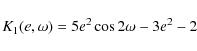
where e and i denote the eccentricity and inclination of the orbiting body, P its period,
Interpreting the observed inclination change as nodal regression due to
an oblate host star, we can compute a lower bound on the required
harmonic coefficient J2 assuming e = 0. Therefore, we combine Eqs. (3) and (5) to obtain an expression for J2. Excluding pathological cases like
![]() and
and
![]() and neglecting the planetary mass in Eq. (5) we find for any given set of parameters
and neglecting the planetary mass in Eq. (5) we find for any given set of parameters
![]()
|
(6) |
where
4.3 Perturbation by a third body
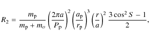
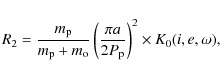
An alternative possibility to explain the observed orbit variations of the TrES-2 exoplanet would be the interaction
with other planets in the system. Let us therefore assume the existence of such an additional perturbing planet of
mass ![]() ,
circling its host star of mass m0 with period
,
circling its host star of mass m0 with period ![]() at distance
at distance ![]() located further out compared to the known transiting TrES-2 exoplanet.
This three-body problem has been considered in past in the context of triple systems (Khaliullin et al. 1991; Li 2006) and
the problem of artificial Earth satellites, whose orbits are perturbed by
the Moon.
In lowest order, the perturbing gravitational potential R2 onto the inner planet with mass m and distance r is given by the expression
located further out compared to the known transiting TrES-2 exoplanet.
This three-body problem has been considered in past in the context of triple systems (Khaliullin et al. 1991; Li 2006) and
the problem of artificial Earth satellites, whose orbits are perturbed by
the Moon.
In lowest order, the perturbing gravitational potential R2 onto the inner planet with mass m and distance r is given by the expression
|
(7) |
where the angle S denotes the elongation between the perturbed and perturbing planet as seen from the host star, a and
|
(8) |
with the auxiliary function
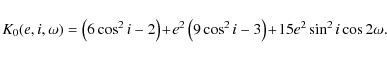
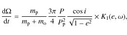
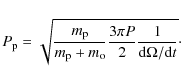
The partial derivatives of R2 with respect to the orbital elements are needed in the so-called Lagrangian planetary equations to derive the variations of the orbital elements of the perturbed body. One specifically finds for the motion of the ascending node
where the auxiliary function
|
(10) |
and for the rate of change of inclination
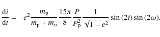
As is obvious from Eq. (11), the rate of change of inclination in low eccentricity systems is very small and we therefore set e = 0. Assuming next a near coplanar geometry, i.e., setting
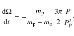
If we assume a host star mass and interpret the observed inclination change as the rate of nodal regression via Eq. (3), Eq. (12) relates the unknown planet mass
4.3.1 Sanity check: application to the solar system
The use of Eq. (12) involves several simplifications. Thus, it is legitimate to ask, if we are justified in expecting Eq. (12) to describe reality. As a sanity
check we apply Eq. (12)
to our solar system. Consider first the motion of the Moon around the Earth, i.e., P = 27.3 d, which is
perturbed by the Sun, i.e.,
![]() d. Since for that case our nomenclature requires
d. Since for that case our nomenclature requires
![]() and
and
![]() ,
we find from Eq. (12)
a time of 17.83 years for the nodes to complete a full circle,
which agrees
well with the canonical value of 18.6 years for the lunar orbit. In the
lunar case it is clear that the Sun with its large mass
and close proximity (compared to Jupiter) is by far the largest
perturber of the Earth-Moon two-body system and this situation is
exactly
the situation described by theory.
,
we find from Eq. (12)
a time of 17.83 years for the nodes to complete a full circle,
which agrees
well with the canonical value of 18.6 years for the lunar orbit. In the
lunar case it is clear that the Sun with its large mass
and close proximity (compared to Jupiter) is by far the largest
perturber of the Earth-Moon two-body system and this situation is
exactly
the situation described by theory.
Consider next the the perturbations caused by the outer planets
of our solar system. Considering, for example, Venus, we can compute
the perturbations caused by the planets Earth, Mars, Jupiter, Saturn
and Uranus. Since the perturbation strength scales
by the ratio
![]() ,
we can set this value to unity for the Earth and compute values of 0.03, 2.26, 0.11 and 0.002
for Mars through Uranus respectively. So clearly, Venus is perturbed by several planets, but the perturbations by Jupiter
are strongest. We therefore expect that our simple approach is not appropriate. We further note that among the outer
solar system planets long period perturbations and resonances occur, which are not described by Eq. (12). If we
nevertheless compute the nodal regression for Venus caused by Jupiter using
Eq. (12), we find a nodal regression of 0.1
,
we can set this value to unity for the Earth and compute values of 0.03, 2.26, 0.11 and 0.002
for Mars through Uranus respectively. So clearly, Venus is perturbed by several planets, but the perturbations by Jupiter
are strongest. We therefore expect that our simple approach is not appropriate. We further note that among the outer
solar system planets long period perturbations and resonances occur, which are not described by Eq. (12). If we
nevertheless compute the nodal regression for Venus caused by Jupiter using
Eq. (12), we find a nodal regression of 0.1![]() /cty for Venus, and 0.3
/cty for Venus, and 0.3![]() /cty for Mars.
Using the orbital elements computed by Simon et al. (1994) and calculating the nodal regressions of Venus and Mars
in the orbit plane of Jupiter we find values smaller than the true values,
but at least, they computed values in the right order of magnitude and do not lead to an overprediction of the expected effects.
/cty for Mars.
Using the orbital elements computed by Simon et al. (1994) and calculating the nodal regressions of Venus and Mars
in the orbit plane of Jupiter we find values smaller than the true values,
but at least, they computed values in the right order of magnitude and do not lead to an overprediction of the expected effects.
4.3.2 Sanity check: application to V 907 Sco
From archival studies Lacy et al. (1999) report the existence of transient eclipses in the triple star V 907 Sco. According to
Lacy et al. (1999) this system is composed out of a short-period (
![]() days) binary containing two main sequence
stars of spectral type
days) binary containing two main sequence
stars of spectral type ![]() A0 and mass ratio 0.9, orbited by a lower mass third companion (
A0 and mass ratio 0.9, orbited by a lower mass third companion (
![]() days), of
spectral type mid-K or possibly even a white dwarf. The close binary
system showed eclipses from the earliest reported observations in 1899
until about 1918, when the eclipses stopped; eclipses reappeared in
1963 and were observed until about 1986. Interpreting the
appearance of eclipses due to nodal regression, Lacy et al. (1999) derive a nodal period of 68 years for V 907 Sco. Using Eq. (12) and assuming a mass of 2
days), of
spectral type mid-K or possibly even a white dwarf. The close binary
system showed eclipses from the earliest reported observations in 1899
until about 1918, when the eclipses stopped; eclipses reappeared in
1963 and were observed until about 1986. Interpreting the
appearance of eclipses due to nodal regression, Lacy et al. (1999) derive a nodal period of 68 years for V 907 Sco. Using Eq. (12) and assuming a mass of 2 ![]() for the host (
for the host (![]() )
and a mass of 0.5
)
and a mass of 0.5 ![]() for the companion
(
for the companion
(![]() ), we compute a nodal regression period of 47.6 years, which agrees well with the nodal period
estimated by Lacy et al. (1999). We therefore conclude that Eq. (12) also provides a reasonable description of the transient
eclipse observations of V 907 Sco.
), we compute a nodal regression period of 47.6 years, which agrees well with the nodal period
estimated by Lacy et al. (1999). We therefore conclude that Eq. (12) also provides a reasonable description of the transient
eclipse observations of V 907 Sco.
4.3.3 Application to TrES 2
Applying now Eq. (12) to the TrES-2 exoplanet we express the period of the (unknown) perturbing planet
as a function of its also unknown mass through
Since the host star mass and the nodal regression are known, the perturbing mass is the only remaining unknown; we note that Eq. (13) should be correct, as long as there is only one dominant perturber in the system with a low-eccentricity orbit sufficiently far away from the known close-in transiting planet. In Fig. 10 we plot the expected perturber period
![\begin{figure}
\par\includegraphics[width=8cm,clip]{Fig010.eps}
\end{figure}](/articles/aa/full_html/2010/02/aa12910-09/img106.png)
|
Figure 10: Period of hypothesized second planet vs. mass assuming a linear coefficient of unity in Eq. (3) and near coplanarity. |
| Open with DEXTER | |
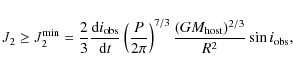
4.4 Transit timing variations by a putative perturber
A perturbing second planet capable of causing fast nodal precession on the transiting planet is also expected to induce short-term periodic variations of its orbital elements. In addition to the secular precession of the node of the orbit we would thus expect to see short-term transit timing variations (TTVs), periodic variations of the mid-transit times (Agol et al. 2005; Holman & Murray 2005). Just as nodal regression, the TTV signal can be used to find and characterize planetary companions of transiting exoplanets. Rabus et al. (2009) carefully analyzed eight transit light curves of TrES-2 over several years. However, they were unable to detect any statistically significant TTV amplitudes in the TrES-2b light curves above about 50 s; cf. their Fig. 10. Therefore, the existence of perturbing objects leading to TTVs on the scale of up to about 50 s are consistent with actual observations. Putting it differently, the orbital parameters of any perturbing object causing the nodal precession of the orbit should yield a TTV amplitude below that and hence remain undetactable in the presently existing data.
To analyze the mutual gravitational influence of a perturbing
second planet in the system on TrES-2, we have to treat the classical
three-body problem of celestial mechanics. Instead of direct N-body
integrations of the equations of motion we use an alternative method
based on analytic perturbation theory developed and extensively tested
by Nesvorný & Morbidelli (2008) and Nesvorný (2009).
Outside possible mean-motion resonances their approach allows for a
fast computation of the expected TTV amplitude given a combination of
system parameters. As input we have to specify the orbital elements and
masses of both planets. Consistent with the observations
we assume TrES-2 to be in a circular orbit around its host star, while
we allow for different eccentricities ![]() and periods
and periods ![]() of the perturber, which we assume to be of Jovian mass; since the TTV
amplitudes scale nearly linearly with the perturber mass, we confine
our treatment to
of the perturber, which we assume to be of Jovian mass; since the TTV
amplitudes scale nearly linearly with the perturber mass, we confine
our treatment to
![]() ;
all other orbital elements are set to zero. This is justified as these
parameters in most cases do not lead to a significant amplification of
the TTV signal (see Nesvorný 2009,
for a detailed discussion of the impact of these orbital elements). The
resulting TTV amplitude for different reasonable orbit configurations
(given the observed secular node regression as discussed above)
of the system of
;
all other orbital elements are set to zero. This is justified as these
parameters in most cases do not lead to a significant amplification of
the TTV signal (see Nesvorný 2009,
for a detailed discussion of the impact of these orbital elements). The
resulting TTV amplitude for different reasonable orbit configurations
(given the observed secular node regression as discussed above)
of the system of
![]() ,
50 and 70 days is plotted vs. the assumed eccentricity in Fig. 11; the currently
available upper limit to any TTV signal derived by Rabus et al. (2009) is also shown. As is obvious from
Fig. 11,
a Jovian-mass perturber at a distance required to impose the observed
secular changes (period of 50-100 days) leads to a TTV signal well
below the current detection limit for all eccentricities
,
50 and 70 days is plotted vs. the assumed eccentricity in Fig. 11; the currently
available upper limit to any TTV signal derived by Rabus et al. (2009) is also shown. As is obvious from
Fig. 11,
a Jovian-mass perturber at a distance required to impose the observed
secular changes (period of 50-100 days) leads to a TTV signal well
below the current detection limit for all eccentricities ![]() as long as
as long as
![]() .
We therefore conclude that a putative perturbing Jovian-mass planet
with a moderate eccentricity and with a period between 30-70 days
would not yield any currently detectable TTV signal and would therefore
be a valid
explanation for the observed inclination change in the TrES-2 system.
.
We therefore conclude that a putative perturbing Jovian-mass planet
with a moderate eccentricity and with a period between 30-70 days
would not yield any currently detectable TTV signal and would therefore
be a valid
explanation for the observed inclination change in the TrES-2 system.
![\begin{figure}
\par\includegraphics[width=7.5cm,clip]{Fig011.eps}
\end{figure}](/articles/aa/full_html/2010/02/aa12910-09/img110.png)
|
Figure 11:
Amplitude of expected Transit Timing Variations (TTVs) in the TrES-2 system. The perturber is assumed to have
|
| Open with DEXTER | |
5 Conclusions
In summary, our new observations taken in the spring of 2009 confirm the smaller transit durations reported in Paper I and suggest an even further decrease. With our simultaneously taken multicolor BUSCA data we demonstrate that the recorded multicolor lightcurves can be consistently modelled with a reasonable set of limb darkening coefficients, and that there is no need to fit the limb darkening coefficients to any particular light curve. An error in the description of the limb darkening therefore appears thus as an unlikely cause of the observed inclination changes. Also as expected, the obtained stellar radius is independent of the wavelength band used, demonstrating the internal self-consistency of our modelling.
As to the possible causes for the observed apparent orbit inclination change in TrES-2 we argue that the apparent observed inclination change is very likely caused by nodal regression. The assumption of an oblate host star leads to implausibly large J2 coefficients, we therefore favor an explanation with a third body. We argue that Eq. (12) is a reasonable approximation for the interpration of the observed inclination changes; applying it to the TrES-2 system, we find that a planet of one Jovian mass with periods between 50-100 days would suffice to cause the observed inclination changes, while at the same time yield TTVs with amplitudes well below the currently available upper limits.
The assumption of such an additional planet in the TrES-2
system is entirely plausible. First of all, if it is near coplanar with
TrES-2b, it would not cause any eclipses and therefore remain
undetected in transit searches. Next, an inspection of the exosolar
planet data base maintained at www.exoplanet.eu
reveals a number of exoplanet systems with properties similar to those
postulated for TrES-2, i.e., a close-in planet together with a massive
planet further out: In the Gl 581 system there is a
0.02 Jupiter-mass planet with a period of 66 days, and in
fact a couple of similarly massive planets further in with periods of
3.1, 5.4 and 12.9 days respectively; in the system HIP 14810
there is a close-in planet with a 6.6 day period and a somewhat
lighter planet with a period of 147 days, in the HD 160691
system the close-in planet has a period of 9.6 days and two outer
planets with Jupiter masses are known with periods of 310 and
643 days. It is also clear that in these systems nodal regression
changes must occur, unless these systems are exactly coplanar, which
appears unlikely. Therefore on longer time scales the observed orbit
inclination in these systems must change, but only in transiting
systems the orbit inclination can be measured
with sufficient accuracy. Because of its apparent inclination change
TrES-2b is clearly among the more interesting extrasolar planets. If
the system continues its behavior in the future the transits of TrES-2b
will disappear. Fortunately, within the first data set of the Kepler
mission ![]() 30 transits should be covered. From our derived inclination change rate of
30 transits should be covered. From our derived inclination change rate of
![]() this corresponds to an overall change of
this corresponds to an overall change of
![]() in this first data set, which ought to be detectable given the superior
accuracy of the space-based Kepler photometry. As far as the detection
of our putative second planet is concerned, RV methods appear to be
more promising than a search for TTVs, unless the orbital
eccentricities are very large.
in this first data set, which ought to be detectable given the superior
accuracy of the space-based Kepler photometry. As far as the detection
of our putative second planet is concerned, RV methods appear to be
more promising than a search for TTVs, unless the orbital
eccentricities are very large.
The paper is based on observations collected with the 2.2 m telescope at the Centro Astronómico Hispano Alemán (CAHA) at Calar Alto (Almería, Spain), operated jointly by the Max-Planck Institut für Astronomie and the Instituto de Astrofísica de Andalucía (CSIC). The authors thank H.Poschmann and the BUSCA team for their tremendous work on the new controller and CCD system. D.M. was supported in the framework of the DFG-funded Research Training Group ``Extrasolar Planets and their Host Stars'' (DFG 1351/1). S.S. acknowledges DLR support through the grant 50OR0703.
References
- Agol, E., Steffen, J., Sari, R., & Clarkson, W. 2005, MNRAS, 359, 567 [NASA ADS] [CrossRef] [Google Scholar]
- Alonso, R., Barbieri, M., Rabus, M., et al. 2008, A&A, 487, L5 [NASA ADS] [CrossRef] [EDP Sciences] [Google Scholar]
- Broucke, R. A. 2003, J. Guidance Control Dynamics, 26, 27 [CrossRef] [Google Scholar]
- Claret, A. 2004, A&A, 428, 1001 [NASA ADS] [CrossRef] [EDP Sciences] [Google Scholar]
- Connon Smith, R. 2005, The Observatory, 125, 341 [NASA ADS] [Google Scholar]
- Daemgen, S., Hormuth, F., Brandner, W., et al. 2009, A&A, 498, 567 [NASA ADS] [CrossRef] [EDP Sciences] [Google Scholar]
- Holman, M. J., & Murray, N. W. 2005, Science, 307, 1288 [NASA ADS] [CrossRef] [PubMed] [Google Scholar]
- Holman, M. J., Winn, J. N., Latham, D. W., et al. 2007, ApJ, 664, 1185 [NASA ADS] [CrossRef] [Google Scholar]
- Howell, S. B., & Everett, M. E. 2001, in Third Workshop on Photometry, ed. W. J. Borucki, & L. E. Lasher, 1 [Google Scholar]
- Khaliullin, K. F., Khodykin, S. A., & Zakharov, A. I. 1991, ApJ, 375, 314 [NASA ADS] [CrossRef] [Google Scholar]
- Kovalevsky, J. 1967, in Les Nouvelles Méthodes de la Dynamique Stellaire, 221 [Google Scholar]
- Lacy, C. H. S., Helt, B. E., & Vaz, L. P. R. 1999, AJ, 117, 541 [NASA ADS] [CrossRef] [Google Scholar]
- Li, L. 2006, AJ, 131, 994 [NASA ADS] [CrossRef] [Google Scholar]
- Miralda-Escudé, J. 2002, ApJ, 564, 60 [NASA ADS] [CrossRef] [Google Scholar]
- Mislis, D., & Schmitt, J. H. M. M. 2009, A&A, 500, L45 [NASA ADS] [CrossRef] [EDP Sciences] [Google Scholar]
- Neckel, H. 1995, Sol. Phys., 156, 7 [Google Scholar]
- Nesvorný, D. 2009, ApJ, 701, 1116 [NASA ADS] [CrossRef] [Google Scholar]
- Nesvorný, D., & Morbidelli, A. 2008, ApJ, 688, 636 [NASA ADS] [CrossRef] [Google Scholar]
- O'Donovan, F. T., Charbonneau, D., Mandushev, G., et al. 2006, ApJ, 651, L61 [NASA ADS] [CrossRef] [Google Scholar]
- O'Donovan, F. T., Charbonneau, D., Harrington, J., et al. 2009, in IAU Symp., 253, 536 [Google Scholar]
- Rabus, M., Deeg, H. J., Alonso, R., Belmonte, J. A., & Almenara, J. M. 2009, A&A, 508, 1011 [NASA ADS] [CrossRef] [EDP Sciences] [Google Scholar]
- Raetz, S., Mugrauer, M., Schmidt, T. O. B., et al. 2009, Astron. Nachr., 330, 459 [NASA ADS] [CrossRef] [Google Scholar]
- Rozelot, J. P., Godier, S., & Lefebvre, S. 2001, Sol. Phys., 198, 223 [NASA ADS] [CrossRef] [Google Scholar]
- Simon, J. L., Bretagnon, P., Chapront, J., et al. 1994, A&A, 282, 663 [NASA ADS] [Google Scholar]
- Sozzetti, A., Torres, G., Charbonneau, D., et al. 2007, ApJ, 664, 1190 [NASA ADS] [CrossRef] [Google Scholar]
Footnotes
- ... exoplanet
- Photometric transit data are only available in electronic form at the CDS via anonymous ftp to cdsarc.u-strasbg.fr (130.79.128.5) or via
http://cdsweb.u-strasbg.fr/cgi-bin/qcat?J/A+A/510/A107
All Tables
Table 1: Observation summary.
Table 2: Relative photometry data.
Table 3:
Individual values of duration, inclination, ![]() values and limb darkening coefficients from five light curve fits.
values and limb darkening coefficients from five light curve fits.
Table 4:
![]() tests for two different inclination values and the
tests for two different inclination values and the ![]() errors after 1000 Monte Carlo simulations.
errors after 1000 Monte Carlo simulations.
All Figures
|
|
Figure 1: Observed TrES-2 light curves and model fits for the light curve taken with the 1.2 m OLT at Hamburg Observatory taken in April 2009. |
| Open with DEXTER | |
| In the text | |
|
|
Figure 2: Four light curves and corresponding model fits taken in May 2009 with the 2.2 m telescope at Calar Alto using BUSCA. |
| Open with DEXTER | |
| In the text | |
|
|
Figure 3: Inclination distribution for the OLT data using 1000 Monte Carlo simulations for the September 2008 (solid curve) and April 2009 (dashed curve); see the text for details. |
| Open with DEXTER | |
| In the text | |
|
|
Figure 4:
Inclination distribution derived 1000 Monte Carlo simulations for the multi-band BUSCA observations data in the I (crosses), y (stars), b (diamonds) and v ( |
| Open with DEXTER | |
| In the text | |
|
|
Figure 5: Stellar radius distribution (R*), derived from 1000 Monte Carlo simulations in four different filters (from higher to lower peak, I, y, b and v filter respectively). The overlap of the curves shows that all colors can be explained with the same stellar radius as suggested by theory (see Neckel 1995). |
| Open with DEXTER | |
| In the text | |
|
|
Figure 6: Epoch versus inclination together with a linear fit to the currently available data; the diamond points are those taken in 2006 by Holman et al. (2007), and those taken in 2008 and reported in Paper I. The square points are derived from our new observations taken in April and May 2009. The solid lines showing two linear fits, from the first paper (dashed line) and the fit from the present paper (solid line). |
| Open with DEXTER | |
| In the text | |
|
|
Figure 7: O-C values versus epoch including the transits observed by Holman et al., Rabus et al. and our data denoted by triangles, squares and diamonds respectively. |
| Open with DEXTER | |
| In the text | |
|
|
Figure 8:
System geometry (see text for details): the orbit plane with normal vector
|
| Open with DEXTER | |
| In the text | |
|
|
Figure 9:
Linear coefficient of Eq. (3) between nodal regression and observed inclination change as a function of view geometry
(cf., Eq. (3)), computed for
|
| Open with DEXTER | |
| In the text | |
|
|
Figure 10: Period of hypothesized second planet vs. mass assuming a linear coefficient of unity in Eq. (3) and near coplanarity. |
| Open with DEXTER | |
| In the text | |
|
|
Figure 11:
Amplitude of expected Transit Timing Variations (TTVs) in the TrES-2 system. The perturber is assumed to have
|
| Open with DEXTER | |
| In the text | |
Copyright ESO 2010
Current usage metrics show cumulative count of Article Views (full-text article views including HTML views, PDF and ePub downloads, according to the available data) and Abstracts Views on Vision4Press platform.
Data correspond to usage on the plateform after 2015. The current usage metrics is available 48-96 hours after online publication and is updated daily on week days.
Initial download of the metrics may take a while.