| Issue |
A&A
Volume 510, February 2010
|
|
|---|---|---|
| Article Number | A103 | |
| Number of page(s) | 25 | |
| Section | Galactic structure, stellar clusters, and populations | |
| DOI | https://doi.org/10.1051/0004-6361/200912836 | |
| Published online | 18 February 2010 | |
Large and small-scale structures of the local Galactic disc
A maximum entropy approach to the stellar velocity distribution
R. Cubarsi
Dept. Matemàtica Aplicada IV, Universitat Politècnica de Catalunya, 08034 Barcelona, Catalonia, Spain
Received 6 July 2009 / Accepted 10 December 2009
Abstract
An analytical model based on the maximum entropy approach is
proposed to describe the eventual asymmetries of the velocity
distribution, which are collected through its sample moments.
If an extended set of moments is available, the current method
provides a linear algorithm, associated with a Gramian system of
equations, that leads to a fast and suitable estimation of the velocity
distribution. In particular, it could be used to model
multimodal distributions that cannot be described through Gaussian
mixtures. The method is used with several samples from the HIPPARCOS
and Geneva-Copenhagen survey catalogues. For the large-scale
distribution, the phase density function may be obtained by fitting
moments up to sixth order as a product of two exponential functions,
one giving a background ellipsoidal shape of the distribution and the
other accounting for the skewness and for the slight shift in the
ellipsoidal isocontours in terms of the rotation velocity. The
small-scale distribution can be deduced from truncated distributions,
such as velocity-bounded samples with
![]() km s-1,
which contain a complex mixture of early-type and young disc stars.
By fitting up to ten-order moments, the maximum entropy approach
gives a realistic portrait of actual asymmetries, showing a clear
bimodal pattern: (i) around the Hyades-Pleiades stream, with
negative radial mean velocity and (ii) around the Sirius-UMa
stream, with slightly positive radial mean velocity. Among metallicity,
colour, and other star properties,
the eccentricity of the star's orbit behaves as a very good sampling
parameter to find a more detailed structure for the disc velocity
distribution, allowing distinctions between different eccentricity
layers. For subsamples with eccentricities e<0.15,
star velocities are approximately symmetrically distributed around the
LSR in the radial direction, with a dearth of stars at the LSR.
For e=0.15, the core distribution of the thin disc is supported
by two major stellar groups with opposite radial velocities. Several
simulations confirm that such a double-peaked distribution comes from
the lognormal distribution of the velocity amplitudes. For maximum
eccentricity 0.3 and maximum distance to the Galactic plane
0.5 kpc a representative thin disc sample is obtained. The
``U-anomaly'' along the radial direction is estimated straightforwardly
30-35 km s-1
from the contour plots. An explanation of the apparent vertex
deviation of the disc from the swinging of those major kinematic groups
around the LSR is then possible,
which predicts a continuously changing orientation of the disc's pseudo
ellipsoid.
km s-1,
which contain a complex mixture of early-type and young disc stars.
By fitting up to ten-order moments, the maximum entropy approach
gives a realistic portrait of actual asymmetries, showing a clear
bimodal pattern: (i) around the Hyades-Pleiades stream, with
negative radial mean velocity and (ii) around the Sirius-UMa
stream, with slightly positive radial mean velocity. Among metallicity,
colour, and other star properties,
the eccentricity of the star's orbit behaves as a very good sampling
parameter to find a more detailed structure for the disc velocity
distribution, allowing distinctions between different eccentricity
layers. For subsamples with eccentricities e<0.15,
star velocities are approximately symmetrically distributed around the
LSR in the radial direction, with a dearth of stars at the LSR.
For e=0.15, the core distribution of the thin disc is supported
by two major stellar groups with opposite radial velocities. Several
simulations confirm that such a double-peaked distribution comes from
the lognormal distribution of the velocity amplitudes. For maximum
eccentricity 0.3 and maximum distance to the Galactic plane
0.5 kpc a representative thin disc sample is obtained. The
``U-anomaly'' along the radial direction is estimated straightforwardly
30-35 km s-1
from the contour plots. An explanation of the apparent vertex
deviation of the disc from the swinging of those major kinematic groups
around the LSR is then possible,
which predicts a continuously changing orientation of the disc's pseudo
ellipsoid.
Key words: stars: kinematics and dynamics - Galaxy: kinematics and dynamics - galaxies: statistics - methods: statistical
1 Introduction
The asymmetry of the local velocity distribution was first studied in 1905 by Kapteyn in his theory of two star streams and further developed by Kapteyn (1922), Strömberg (1925), and Charlier (1926), which considered up to fourth moments of the velocity distribution. However, those moments were not determined with a sufficient degree of accuracy up to Erickson (1975). During the past decade, higher order velocity moments with better precision could be obtained from large and representative stellar samples of the solar neighbourhood, like the HIPPARCOS calatogue (ESA 1997) or, more recently, the Geneva-Copenhagen Survey (GCS) (Nordtröm et al. 2004), accounting for velocity discontinuities and kinematic populations in the solar neighbourhood (Cubarsi & Alcobé 2004; Alcobé & Cubarsi 2005). Several approaches have been tried to describe the asymmetry of the velocity distribution. In the beginning, an anisotropic velocity distribution was obtained by superposition of isotropic phase-density functions with different means. Later, the Schwarzschild distribution, based on a single trivariate Gaussian distribution, could easily handle the basic anisotropic features, and more parameters could be controlled by assuming non-Gaussian ellipsoidal distributions. However, to account for non-null, odd-order central moments, it was once again necessary to return to mixture models.
In addition to the works describing the actual velocity distribution from a mixture of stellar populations (e.g. Soubiran & Girard 2005; Vallerani et al. 2006), there is a wide variety of approaches that generally do not make use of the velocity moments, such as the two- or three-integral models based in Fricke (1952) components (Evans et al. 1997; Famaey et al. 2002; Jiang & Ossipkov 2007) or even a combination of a Gaussian part of the density function with a perturbation factor expressed in a polynomial form in terms of the integrals of motion (van der Marel & Franx 1993; Gerhard 1993; Kormendy et al. 1998). The velocity distribution is sometimes numerically estimated (Dehnen 1998; Skuljan et al. 1999; Bovy et al. 2009), although it is also frequently the analytical modelling (Famaey et al. 2005; Veltz et al. 2008). However, in the latter case, according to today's observational data, some intricate trivariate distribution functions (or with a very high number of components) may be obtained. In most of these works, there is the job of describing the detailed structure of the velocity distribution, or of associating specific moving groups with the density function components, although in most cases the small groups do not have a clear visual impact on the overall density function. There is also a desire for a simple, qualitative description of the distribution in terms of basic measures of spread or asymmetry like the skew or for a comparison to Gaussian distributions, like the curtosis. For trivariate distributions with strong asymmetries, e.g. the structure that lies under the groups of young and early-type stars, the statistical moments are the natural tool for such a description of the basic geometric trends. To this purpose, the method of moments is revisited here.
An alternative analytical model based on the maximum entropy approach is proposed to describe the eventual asymmetries of the velocity distribution, which are collected through its sample moments. Even though such an approach has been widely used to solve many univariate technical and scientific problems, to my knowledge there has been no general application to stellar kinematics. There are several numeric algorithms for estimating the maximum entropy density function, which are not computationally trivial for the trivariate case. However, if an extended set of moments is available, the method described in this work allows a parameter estimation by solving a linear system of equations. Its simplicity makes it worthwhile using it to construct any ad hoc velocity distribution function.
The maximum entropy approach will be used to describe the main kinematical features of solar neighbourhood stars by working from the two formerly mentioned large and kinematically representative local stellar samples. In the first case, the large-scale distribution of the local disc is inferred from Sample I (Cubarsi & Alcobé 2004), obtained by crossing the HIPPARCOS Catalogue with radial velocities from the HIPPARCOS Input Catalogue (ESA 1992). In the second case, the method is applied to Sample II from the GCS catalogue. It has new and more accurate radial velocity data than the HIPPARCOS sample, and contains the total velocity space of F and G dwarf stars, which are considered the favourite tracer populations of the history of the disc. In both cases, the largest samples providing stable velocity moments are used. The preceding applications provide and confirm some general and well known trends in the background velocity distribution, such as the overall vertex deviation, the skewness, or the symmetry plane of the distribution. These stellar samples, which mainly contain thin and thick disc stars, can be sufficiently described from an exponential density function with a four-degree polynomial, although a six-degree polynomial provides a more accurate portrait of the local velocity distribution. According to the maximum entropy modelling, it is possible to interpret the velocity distribution as a product of two exponential functions, the one giving a background ellipsoidal shape of the distribution and the other, which is even and at least quadratic in the rotation velocity alone, acting as a perturbation factor that breaks the distribution symmetry.
On the other hand, the small-scale velocity distribution of the local
disc can be deduced from truncated distributions. According to Alcobé
& Cubarsi (2005), hereafter Paper I, a selection of stars with an absolute value of the total space motion
![]() km s-1
leaves the older disc stars aside. Such a selection is analysed in
more depth and their properties described better. It contains a
complex mixture of early-type and young disc stars for which
a Gaussian mixture approach is not feasible. Thus, Sample III
is built as a subsample of Sample I with
km s-1
leaves the older disc stars aside. Such a selection is analysed in
more depth and their properties described better. It contains a
complex mixture of early-type and young disc stars for which
a Gaussian mixture approach is not feasible. Thus, Sample III
is built as a subsample of Sample I with
![]() km s-1. Finally, Sample IV is drawn from Sample II under the same condition on the absolute velocity.
km s-1. Finally, Sample IV is drawn from Sample II under the same condition on the absolute velocity.
It is also possible to obtain a more detailed structure of the velocity distribution for specific subsamples, allowing the results of our approach to be compared with the small-scale structure sustained by moving groups. Among metallicity, colour, and other star properties, the eccentricity of the star's orbit is found to behave as a very good sampling parameter that allows distinguishing between different eccentricity layers within the thin disc, and allowing visualisation of the underlying structure of the distribution. In particular, for maximum eccentricity 0.3 and maximum distance to the Galactic plane 0.5 kpc, we get a representative thin disc sample.
For these truncated distributions, the density function needs a six-degree polynomial to describe their strong asymmetries and their main kinematic features. The improvement in the GCS catalogue over the HIPPARCOS catalogue provides a higher resolution contour plot for the inner thin disc, which in addition to describing a velocity distribution far from the ellipsoidal hypothesis, explains a clear bimodal structure. Therefore, the maximum entropy modelling can be presented as an alternative way instead of mixture models.
The paper is organised as follows. In Sect. 2 the notation is introduced while reviewing some basic concepts of stellar statistics. Maximum entropy density functions are introduced and the meaning they have in mathematical statistics and statistical mechanics discussed. The mathematical formulation of the current functional approach is developed in Appendix A. In Sect. 3 the method is applied to local stellar samples from the HIPPARCOS and the GCS catalogues, for either complete (large-scale) or truncated (small-scale) distributions. Some aspects of the results and of the subsamples are analysed. In Sect. 4 a link to a dynamical model allows interpretation of the major kinematical groups sustaining the disc structure and of its possible swinging vertex deviation. Finally, in Sect. 5, the conclusions are presented.
2 Method
We study the necessary complexity of the velocity distribution for satisfying a set of moment constraints. The current approach simplifies both analytical dependence and parameter estimation of the distribution function under the following circumstances. We choose a density function maximising Shannon's information entropy. The maximum entropy approach to the solution of inverse problems was introduced long ago by Jaynes (1957a,b), so that it provides a unique solution that is the best one for not having to deal with missing information. It agrees with what is known, but expresses maximum uncertainty with respect to all other matters. It is a flexible and powerful tool for density approximation, which collects a complete family of generalised exponential distributions, including the exponential, normal, lognormal, gamma, and beta as special cases. Other properties of maximum entropy distributions are outlined in Appendix A.
An interesting application of the maximum entropy approach is the problem of moments (Mead & Papanicolaou 1984), which is described along with introducing the notation accordingly to the astronomical formulation.
2.1 Stellar statistics
For fixed values of time t and position ![]() ,
the macroscopic properties of a stellar
system can be described from the moments of the distribution, which
provide indirect information on the phase-space density function
,
the macroscopic properties of a stellar
system can be described from the moments of the distribution, which
provide indirect information on the phase-space density function
![]() ,
which is normalised with regard to the velocities. It is well
known that the first moments, accounting for the mean, give the more
elementary property of the distribution; the second central moments
describe how much the distribution is spread around the mean; the third
moments describe distribution asymmetries like the skewness; the fourth
moments are used to quantify how peaked the distribution is;
and so forth (e.g. Stuart & Ord 1987). In general, the symmetric tensor of the
,
which is normalised with regard to the velocities. It is well
known that the first moments, accounting for the mean, give the more
elementary property of the distribution; the second central moments
describe how much the distribution is spread around the mean; the third
moments describe distribution asymmetries like the skewness; the fourth
moments are used to quantify how peaked the distribution is;
and so forth (e.g. Stuart & Ord 1987). In general, the symmetric tensor of the ![]() -order, non-centred trivariate moments is obtained from the expected value
-order, non-centred trivariate moments is obtained from the expected value
where
so that the indices belong to the set
Obviously, m0=1 and
In a similar way, the symmetric tensor of the ![]() -order centred moments is obtained by working from the peculiar velocity
-order centred moments is obtained by working from the peculiar velocity
defined as
Hereafter, when studying the velocity dependence of the distribution function from a statistical viewpoint, the variables of time and position are omitted, although they might be used in the framework of a dynamical model for the whole phase-space distribution function.
Ellipsoidal distributions, such as the Schwarzschild distribution, can
be described in terms of their central second moments ![]() ,
which sometimes are written with Latin indices, such as
,
which sometimes are written with Latin indices, such as
![]() (e.g. Binney & Tremaine 1987,
pp. 194-211). However, in other standard astronomy reference
books, the Greek index notation is used (e.g. Gilmore et al. 1989, p. 135-138), in particular when the velocity variables are expressed in the (U,V,W) coordinate system (without subindices), where the nth moments
(e.g. Binney & Tremaine 1987,
pp. 194-211). However, in other standard astronomy reference
books, the Greek index notation is used (e.g. Gilmore et al. 1989, p. 135-138), in particular when the velocity variables are expressed in the (U,V,W) coordinate system (without subindices), where the nth moments
![]() satisfy
satisfy
![]() .
The second central moments account for the shape and orientation of the velocity ellipsoid and for the variance
.
The second central moments account for the shape and orientation of the velocity ellipsoid and for the variance
![]() of the velocity distribution function in an arbitrary direction l of the peculiar velocity space. According to the coordinate system, if c1, c2, and c3 are the corresponding direction cosines, we have
of the velocity distribution function in an arbitrary direction l of the peculiar velocity space. According to the coordinate system, if c1, c2, and c3 are the corresponding direction cosines, we have
|
(5) |
The symmetric tensor

|
(6) |
so that the velocity dispersions
2.2 Maximum entropy
Therefore, more general and anisotropic distributions have a wider
set of independent moments, and, in the more general case, the exact
distribution may be univocally determined by the infinite hierarchy of
independent moments. Provided an order for a set of moments
(for example according to the Latin indices notation 0, 1, 2,
3, 11, 12, 13, 22, and so on) if the first m moments are known, it is possible to find an infinite variety of functions whose first m moments coincide with the above set. Various approximation procedures exist to find a sequence of functions fm, which fulfils the foregoing moment constraints and converges to the true distribution as m
approaches infinity. Fortunately, between those sequences of functions,
a uniquely maximum entropy sequence exists that maximises the
entropy functional
Then, the maxima f=fm is usually called the least biassed sequence of approximations, and, by using Lagrangian multipliers, it can be shown (e.g. Kagan et al. 1973) that it has the form

where
The solution of the maximum entropy problem usually consists in solving a set of m nonlinear equations in the form
However, these solution techniques are typically not easy to generalise to the multidimensional problem. On the other hand, even for the unidimensional problem, an analytical solution generally does not exist for higher than second moments. Generally, the numerical techniques for solving the coefficients of the polynomial
Thus, the current purpose is to infer the trivariate velocity
distribution from a finite set of moment constraints. To simplify
estimation of the polynomial coefficients of
![]() ,
an alternative method has been developed, based on a unique
assumption that the velocity distribution satisfies the boundary
conditions associated with the stellar hydrodynamic equations, also
known as moment equations.
,
an alternative method has been developed, based on a unique
assumption that the velocity distribution satisfies the boundary
conditions associated with the stellar hydrodynamic equations, also
known as moment equations.
If the phase-space distribution function f satisfies the collisionless Boltzmann equation,
![]()
![]() , then by multiplying it by the
, then by multiplying it by the ![]() -tensor
power of the star velocity and by integrating over the whole velocity
space, the family of stellar hydrodynamic equations is obtained:
-tensor
power of the star velocity and by integrating over the whole velocity
space, the family of stellar hydrodynamic equations is obtained:
In Cubarsi (2007), the above equations were derived in terms of the central or comoving moments, in a completely analytical way, for any order n and without any additional hypotheses. Then, if the above integrals exist and since there are no stars with velocity beyond
These boundary conditions are satisfied by a wide family of distributions that are bell-shaped in any direction of the velocity domain. One of the integral properties that was derived in Cubarsi (2007) will allow, in Appendix A.1, establishment of a Gramian system of equations for solving our estimation problem. From a purely statistical inference viewpoint, the requirement of estimating the distribution parameters is not that the phase density function is the solution to the collisionless Boltzmann equation, but it is enough that it satisfies, or approximately satisfies, the above boundary conditions.
The entropy functional W(f), as defined in Eq. (7), is far from containing all the information about the Boltzmann equation (with or without collisions) since W(f) only depends on the velocity space, similar to the collision operator of the complete Boltzmann equation. In the following section, we discuss how such a maximum entropy density function may or may not be a solution to the collisionless Boltzmann equation.
In review, two typical cases of maximum entropy distribution
function are solutions to the whole set of moment equations. The
simplest case is an isothermal velocity distribution of Maxwell type in
the peculiar velocities, which according to the
Maxwell-Boltzmann law, represents a system with the more basic
thermal equilibrium
where
Another well known example is the Schwarzschild distribution, that is,
an exponential density function that depends on the peculiar
velocities in a quadratic way (Chandrasekhar 1942),
where Q is a quadratic, positive-definite form, with
The above examples, which are integrable functions in an infinite velocity domain, satisfy the boundary conditions, Eq. (11), and can be generalised according to an exponential function, Eq. (8),
with as many polynomial terms as available moment constraints, under
the necessary conditions over the polynomial coefficients to obtain an
integrable distribution function. For higher-degree polynomials, the
distribution function is integrable if the polynomial is upper bounded,
and therefore the polynomial must be even. On the other hand, truncated
distributions, which are associated with velocity-bounded stellar
samples,
![]() ,
have a finite velocity domain. Then the boundary conditions are still a
good approximation if the truncated distribution vanishes enough when
approaching the contour of the velocity domain, so that the
density function may be assumed null out of this boundary. Thus, for a
domain that is either bounded or unbounded, we assume that the velocity
distribution is continuous, differentiable, and positive in the
interior of the velocity domain
,
have a finite velocity domain. Then the boundary conditions are still a
good approximation if the truncated distribution vanishes enough when
approaching the contour of the velocity domain, so that the
density function may be assumed null out of this boundary. Thus, for a
domain that is either bounded or unbounded, we assume that the velocity
distribution is continuous, differentiable, and positive in the
interior of the velocity domain ![]() and that the boundary conditions are fulfiled in its contour
and that the boundary conditions are fulfiled in its contour
![]() .
.
2.3 Information entropy
Let us briefly explain how to interpret a maximum entropy density function, or better, what is the appropriate context for its use. Up to a change of sign, Shannon's information entropy is defined as the Boltzmann H-functional, which first appeared in statistical mechanics in works by Boltzmann and Gibbs in the 19th century. However, it is not exactly the same concept.
Boltzmann's functional is used for non-equilibrium systems and is related to the irreversibility of dynamical processes in a uniform gas. For elastic collisions involving short-range forces and in the absence of boundaries, mass, momentum, and energy are conserved in binary encounters (e.g. Cercignani 1988). They are usually referred to as collisional invariants. There is only one distribution function, the Maxwellian distribution, fulfiling all of the following properties: it depends on a linear combination of the collisional invariants, the collision term of the Boltzmann equation is exactly zero, and it minimises Boltzmann's entropy. This solution represents a local equilibrium state, in the sense that other solutions to the Boltzmann equation will become closer to it as the time goes by. Depending on the potential, boundary conditions, and dissipative or collision effects (e.g. Villani 2002), maximum entropy solutions can be non-Maxwellian.
Shannon's information entropy![]() was introduced in communication theory to measure the redundancy of a
language and the maximal compression rate, which is applicable to a
message without any loss of information. It is defined for complex
systems and is related to Boltzmann's entropy as a measure of the
number of microstates associated with a given macroscopic
configuration. On the other hand, the Fisher information was introduced
as part of his theory of coefficient statistics as a measure of the
uncertainty. It is also related to Shannon's entropy, so that
the entropy quantifies the variation of information. If we
maximise the entropy subject to some constraints (e.g. statistics
describing macroscopic properties) we get distributions containing
maximum uncertainty that is compatible with these constraints.
was introduced in communication theory to measure the redundancy of a
language and the maximal compression rate, which is applicable to a
message without any loss of information. It is defined for complex
systems and is related to Boltzmann's entropy as a measure of the
number of microstates associated with a given macroscopic
configuration. On the other hand, the Fisher information was introduced
as part of his theory of coefficient statistics as a measure of the
uncertainty. It is also related to Shannon's entropy, so that
the entropy quantifies the variation of information. If we
maximise the entropy subject to some constraints (e.g. statistics
describing macroscopic properties) we get distributions containing
maximum uncertainty that is compatible with these constraints.
For given mass and energy, the Fisher information takes its minimum value and Shannon's entropy its maximum value in the form of Maxwellian distributions. For a given covariance matrix, they take extreme values for Gaussian distributions. The number of constraints involved in the Lagrange multipliers may reach higher order moments, by reflecting more complex situations in which the stars interact with the potential and with themselves, as well as having different masses.
We quote Jaworsky (1987) to point out that these two typical viewpoints for interpreting the entropy as uncertainty. In mathematical statistics and information theory, the entropy functional is maximised by attending to some constraints that express any available information of a complex physical system, which depend on the actual experimental situation. In statistical mechanics the entropy is used to study the thermodynamic equilibrium or non-equilibrium of a physical system, generally a uniform gas, in terms of the mean values of some physical quantities, which describe the macroscopic state of a physical system as a whole, like energy or number of particles. Thus, statistical mechanics based on this principle can be interpreted as a special type of statistical inference. The use of higher order statistical moments in addition to the mean values represents a generalisation of the thermodynamic concept of entropy, which is used to approximate the exact probability distributions for a few specified random variables when a finite number of their moments is known.
The maximum entropy principle implies that the the resulting
distribution belongs to the exponential family. The actual moment
constraints are a direct consequence of the isolating integrals of the
stellar motion, or more precisely, they reflect particular
combinations of the isolating integrals that are conserved. More
complex distributions exist than the Maxwellian, which are maximum
entropy distributions and are solution of the collisionless Boltzmann
equation. These solutions are generally obtained by assuming that
Liouville's theorem is satisfied, so that the essential
information about the density function is provided by the isolating
integrals of the motion of the stars. Thus, if we assume that the
polynomial form ![]() of Eq. (7)
depends on the integrals of motion and is itself an integral of motion,
Liouville's theorem is equivalent to the collisionless Boltzmann
approximation. Then, the collisionless Boltzmann equation obviously
takes the form
of Eq. (7)
depends on the integrals of motion and is itself an integral of motion,
Liouville's theorem is equivalent to the collisionless Boltzmann
approximation. Then, the collisionless Boltzmann equation obviously
takes the form

|
(14) |
so that the factor
The physical mechanism providing such a maximum entropy function is
irrelevant to the statistical approach. In contrast, what is
important is the set of statistical moments accounting for the
macroscopic state, which, of course, have a dynamical significance
in terms of viscosity, conductivity, or diffusion effects. The
present statistical approach adopts the opposite viewpoint of studying
possible warming mechanisms that modify a Schwarzschild distribution,
and to then test how the distribution fits the actual velocity moments
(e.g. Dehnen 1999). In the current method, the available information is condensed within the polynomial
![]() .
The maximum entropy approach then gives a very good mathematical
estimation of the density function and of its velocity derivatives
involved in
.
The maximum entropy approach then gives a very good mathematical
estimation of the density function and of its velocity derivatives
involved in
![]() ,
although it may or may not match any physical model. On the other hand,
the maximum uncertainty in the light of the missing information is
guaranteed by the function
,
although it may or may not match any physical model. On the other hand,
the maximum uncertainty in the light of the missing information is
guaranteed by the function
![]() .
.
The maximum entropy density function may be explicitly written as
where the subindex n does not represent the number of polynomial terms, but rather the maximum polynomial power.
If the velocity domain ![]() is all the space R3, the polynomial
is all the space R3, the polynomial
![]() must
be upper bounded to satisfy the integrability conditions. As a
result, the power series of the velocities reaches a natural value n, which must be even, and, for the highest degree k=n, the n-adic form
must
be upper bounded to satisfy the integrability conditions. As a
result, the power series of the velocities reaches a natural value n, which must be even, and, for the highest degree k=n, the n-adic form
![]() must be negative definite.
must be negative definite.
|
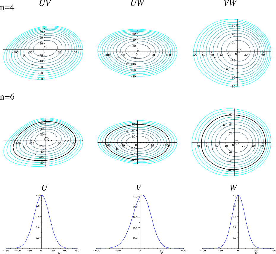
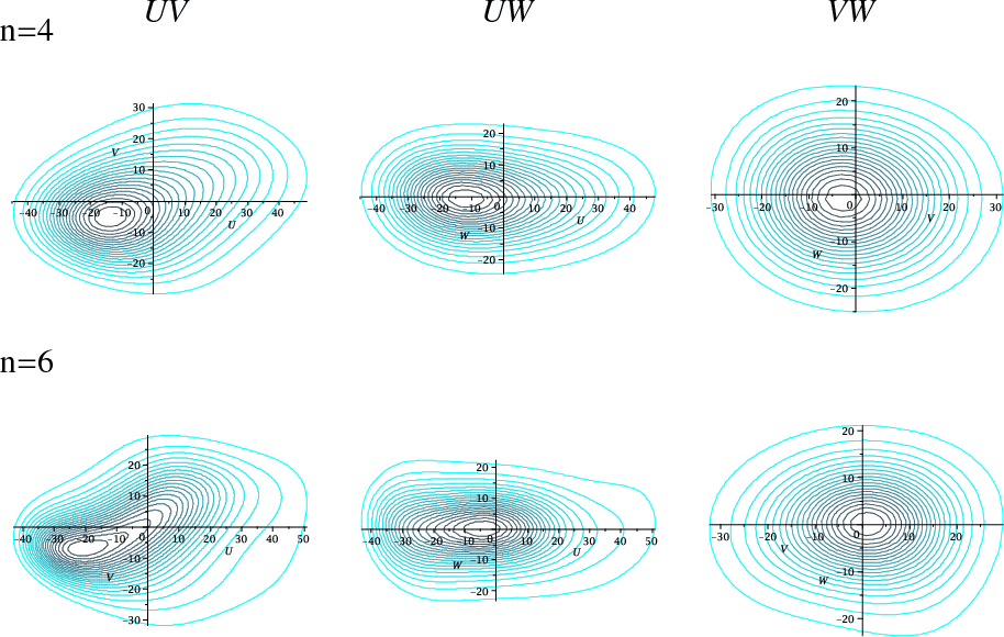
Figure 1:
Contour plots of the local velocity distribution in terms of the
peculiar velocities for HIPPARCOS' Sample I and Sample I'.
The plots are centred on the mean heliocentric velocity
(-10.85, -19.93, -7.49) km s -1 of Sample I', with radial velocity errors up to 2.5 km s-1. The case n=4, by fitting up to sixth moments, leads to more realistic contour plots than a pure ellipsoidal distribution (n=2), although n=6 provides a slightly improvement, by fitting up to tenth moments. The contours indicate levels
|
| Open with DEXTER | |
Equation (15), in addition to including Eqs. (12) and (13) as particular cases, also contains, in general, any desired type of two- or three-integral functions (e.g. Hénon 1973; Dejonghe 1983; White 1985). It represents a general functional approach, in a similar way to Fricke (1952), with the difference that, while the distribution function in the Fricke-based models is either a linear combination or product of the powers of integrals of motion, in Eq. (15) the linear combination of powers of integrals of motion appears as the argument in the exponential function.
The mathematical formulation of the maximum entropy functional approach
is detailed in Appendix A. The smoothest density function that is
consistent with an extended set of moment constraints is provided by
the Gramian system of equations in Eq. (42). The resulting system allows computation of the elements of tensors
![]() in terms of the velocity moments up to order 2(n-1), which is the highest order involved in Eq. (40), as discussed in Appendix A.2. For the case n=2,
it is easy to solve the Gramian system in an analytical way and to
find out how moments of order higher than two depend on the second ones
(Appendix B). For higher values of n, however, it must be done by using the numerical procedure
outlined in Appendix A.3. Also, for n=2, the integrability of the distribution function in an infinite velocity domain is easily derived from the tensor
in terms of the velocity moments up to order 2(n-1), which is the highest order involved in Eq. (40), as discussed in Appendix A.2. For the case n=2,
it is easy to solve the Gramian system in an analytical way and to
find out how moments of order higher than two depend on the second ones
(Appendix B). For higher values of n, however, it must be done by using the numerical procedure
outlined in Appendix A.3. Also, for n=2, the integrability of the distribution function in an infinite velocity domain is easily derived from the tensor
![]() ,
since
,
since
![]() ,
where the tensor of second central moments
,
where the tensor of second central moments
![]() is positive-definite. For
is positive-definite. For ![]() ,
it is impossible to guarantee the definiteness of the tensor
,
it is impossible to guarantee the definiteness of the tensor
![]() in a general way. This is a problem related to Hilbert's 17th
problem,
which is obviously beyond the scope of the present work. However,
by using a finite velocity domain, one as wide as needed,
according to the working stellar sample, such a problem may be
easily avoided for truncated distributions, as described
in Appendix A.1.
in a general way. This is a problem related to Hilbert's 17th
problem,
which is obviously beyond the scope of the present work. However,
by using a finite velocity domain, one as wide as needed,
according to the working stellar sample, such a problem may be
easily avoided for truncated distributions, as described
in Appendix A.1.
3 Application
Several illustrations of the current functional approach are used to
describe the main kinematical features of the solar neighbourhood. The
first two cases give the whole velocity distribution of the local disc,
which is usually fitted by a mixture of trivariate Gaussian
distributions. In the first application, a nearly complete
and kinematically representative local sample, Sample I (Cubarsi
& Alcobé 2004) with 13 678 stars, is used. It was obtained by crossing the HIPPARCOS Catalogue (ESA 1997) with radial velocities from the HIPPARCOS Input Catalogue (ESA 1992).
To get a representative sample of the solar neighbourhood,
it was limited to a trigonometric distance of 300 pc, where
the only input data points were the velocity components (U,V,W) in a cartesian heliocentric coordinate system, with U toward the Galactic centre, V in the rotational direction, and W perpendicular
to Galactic plane, positive in the direction of the North Galactic
pole. In Paper I it was found that the optimal subsample
containing thin and thick disc stars could be obtained by selecting
stars with absolute heliocentric velocity
![]() km s-1. The sample has undergone a deeper statistical analysis in Cubarsi et al. (2010), hereafter Paper II, where the subsamples selected from
km s-1. The sample has undergone a deeper statistical analysis in Cubarsi et al. (2010), hereafter Paper II, where the subsamples selected from
![]() km s-1
contain, in addition to above disc populations, a fraction up
to 1% of halo stars, with very stable computed moments.
To compare results with the next sample, the velocity domain is
limited to the absolute space velocity of 500 km s-1,
which only excludes five stars from the whole sample. The resulting
Sample I is then composed of 13 673 stars. The
distribution smoothly vanishes in reaching the velocity boundary,
as shown in the last row of Fig. 1. For all practical purposes, the sample may be considered as unbounded. To compare between different fittings, Eq. (42) up to n=6 is used, by taking up to tenth moments into account. According to Appendix A.3, by normalising to the number N of equations, the squared error of the fit is then given by the expression
km s-1
contain, in addition to above disc populations, a fraction up
to 1% of halo stars, with very stable computed moments.
To compare results with the next sample, the velocity domain is
limited to the absolute space velocity of 500 km s-1,
which only excludes five stars from the whole sample. The resulting
Sample I is then composed of 13 673 stars. The
distribution smoothly vanishes in reaching the velocity boundary,
as shown in the last row of Fig. 1. For all practical purposes, the sample may be considered as unbounded. To compare between different fittings, Eq. (42) up to n=6 is used, by taking up to tenth moments into account. According to Appendix A.3, by normalising to the number N of equations, the squared error of the fit is then given by the expression
The maximum entropy procedure with n=2 tries to represent the whole distribution from an unique ellipsoidal distribution. Thus, odd-order moments and even-order moments higher than four are not fitted. The resulting fitting error
In a second example, the method is applied to Sample II, drawn
from the GCS catalogue (Nordtröm et al. 2004; Holmberg
et al. 2007).
It has new and more accurate radial velocity data than the
HIPPARCOS sample and contains the total velocity space of
13 240 F and G dwarf stars, which are considered the
favourite tracer populations of the history of the disc. According to
the authors, the main essential features of the sample are the lack of
kinematic selection bias and the radial velocity data, which allowed to
reject stars that have not taken part in the evolution of the local
disc. The same cartesian heliocentric coordinate system is used. For
this sample, according to the analysis in Paper II, the moments
are computationally stable for all the velocity components in the range
![]() km s-1. The limitation up to an absolute velocity space of 500 km s-1
excludes five stars. The halo component is present in the total sample
in a fraction less than 0.5%. Therefore, for practical purposes,
this sample may also be considered as unbounded. The results and the
graphs are similar to those of Sample I.
km s-1. The limitation up to an absolute velocity space of 500 km s-1
excludes five stars. The halo component is present in the total sample
in a fraction less than 0.5%. Therefore, for practical purposes,
this sample may also be considered as unbounded. The results and the
graphs are similar to those of Sample I.
In the next section we confirm that the GCS sample provides more
accurate moments of the disc velocity distribution than HIPPARCOS' due
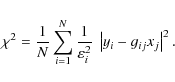
to its more precise radial velocities. In Table 1,
centred and non-centred velocity moments up to order four are listed
for the GCS Sample II, along with their standard errors. These are
moments for a mixture of thin disc (94%), tick disc (5.5%),
and halo (0.5%), as discussed in Paper II. They allow
some measures of spread and asymmetry of the distribution in the
desired variables to be computed, as the non null skewness in the
rotation velocity V,
![]()
![]() 0.5 (in the Greek indices notation), which is zero in the other
components. The moments also lead to a non-significant curtosis in the
vertical velocity W,
0.5 (in the Greek indices notation), which is zero in the other
components. The moments also lead to a non-significant curtosis in the
vertical velocity W,
![]()
![]() 40, or the non-vanishing vertex deviation on the UV plane
40, or the non-vanishing vertex deviation on the UV plane
![]()
![]() 2.3.
2.3.
Therefore, the main features of the maximum entropy distribution for Samples I and II, which show a reasonable deviation from an ellipsoidal distribution, may be easily deduced from Fig. 1, either for n=4 or n=6. The main features are:
- (i)
- the velocity distribution is not symmetric around the mean, mainly in the rotation direction;
- (ii)
- the whole distribution has a clear vertex deviation on the plane UV and no deviation on other planes;
- (iii)
- there is some skewness in the variable V. As a consequence of both previous situations there is a wider distribution wing towards lower U and V velocities, which is likely caused by thick disc stars;
- (iv)
- the curtosis in the W variable vanishes and is zero or very small in the U velocity (see Table 3);
- (v)
- the plane W=0 is basically a symmetry plane.
where Q is a quadratic negative-definite form, which gives the background ellipsoidal shape of the distribution, with axis ratios 1:0.7:0.5, symmetry plane W=0, as expected for disc stellar samples, and overall vertex deviation in the UV velocity components of about
Table 1:
Centred moments
![]() and non-centred moments
and non-centred moments
![]() with their standard errors up to fourth order for the GCS Sample II.
with their standard errors up to fourth order for the GCS Sample II.
The bulk of the local velocity distribution does not show any substructure reflecting the existing moving groups, even by associating these moving groups with different proxy Gaussian components (Bovy et al. 2009). Then, it results in a smooth background distribution. However, by selecting specific subsamples by colour, or by using different analysis techniques where the resolution scale may vary, the substructures of the velocity distribution arise. We discuss it in the next section.
|
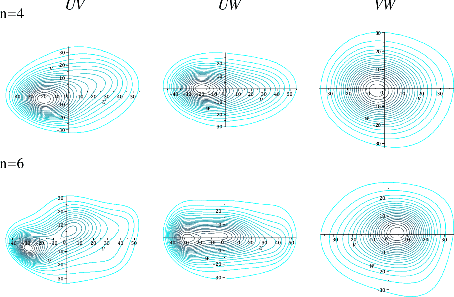
Figure 2:
Contour plots of the velocity distribution for Sample III, from the HIPPARCOS catalogue, for stars with
|
| Open with DEXTER | |
|
Figure 3:
Contour plots of the velocity distribution for Sample IV, from the GCS catalogue, with
|
| Open with DEXTER | |
The next two examples are used for two new purposes: first, to test
the ability of the maximum entropy method in reconstructing a truncated
velocity distribution associated with a velocity bounded sample;
second, to try a magnifying glass effect over the distribution and
to focus on a specific velocity domain. According to Paper I, the
selection of local stars with an absolute value of the total space
motion
![]() km s-1
had left the older disc stars aside, which are the originators of an
important softening of the distribution. Such a selected group of
stars contained a complex mixture of early-type and young disc stars
for which a Gaussian mixture approach was unreliable because of
the large fitting errors. This small-scale structure of the velocity
distribution was strongly asymmetric in comparison to the background
distribution. It was also observed in other analyses of the solar
neighbourhood (e.g. Famaey et al. 2005; Soubiran & Girard 2005).
km s-1
had left the older disc stars aside, which are the originators of an
important softening of the distribution. Such a selected group of
stars contained a complex mixture of early-type and young disc stars
for which a Gaussian mixture approach was unreliable because of
the large fitting errors. This small-scale structure of the velocity
distribution was strongly asymmetric in comparison to the background
distribution. It was also observed in other analyses of the solar
neighbourhood (e.g. Famaey et al. 2005; Soubiran & Girard 2005).
Sample III is then composed of 10 195 stars from the HIPPARCOS Sample I, with
![]() km s-1. The maximum entropy approach for n=2 gives a fitting error
km s-1. The maximum entropy approach for n=2 gives a fitting error
![]() ,
according to Eq. (16).
Although it could seem a very low value compared to previous samples,
we might bear in mind that Samples I and II contain stars
with higher velocity than Sample III, which increases the
uncertainty of the computed moments. Because of this, the fitting
errors for Sample III are expected to be much smaller. Once again,
we must pay attention to the variation in
,
according to Eq. (16).
Although it could seem a very low value compared to previous samples,
we might bear in mind that Samples I and II contain stars
with higher velocity than Sample III, which increases the
uncertainty of the computed moments. Because of this, the fitting
errors for Sample III are expected to be much smaller. Once again,
we must pay attention to the variation in ![]() .
.
For n=4, the approach is able to provide a more realistic, non-ellipsoidal map of the truncated
distribution by fitting moments up to sixth order. In this case the fitting error is
![]() .
Nevertheless, for n=6, the maximum entropy approach gives a much improved portrait by fitting up to tenth moments. The fitting error
.
Nevertheless, for n=6, the maximum entropy approach gives a much improved portrait by fitting up to tenth moments. The fitting error
![]() is about 102 times
lower than the ellipsoidal approach. The contour plots of the velocity
distribution on each velocity plane are displayed in Fig. 2. The coordinate system is centred in the heliocentric mean velocity
(-7.49, -11.25, -6.41) km s-1.
is about 102 times
lower than the ellipsoidal approach. The contour plots of the velocity
distribution on each velocity plane are displayed in Fig. 2. The coordinate system is centred in the heliocentric mean velocity
(-7.49, -11.25, -6.41) km s-1.
Finally, Sample IV is drawn from the GCS catalogue by selecting
9733 stars with absolute velocity lower than 51 km s-1. As in the above example, the approaches with n=2 (
![]() )
and n=4 (
)
and n=4 (
![]() )
are not able to provide a realistic map of the truncated distribution. However, for n=6, with a fitting error
)
are not able to provide a realistic map of the truncated distribution. However, for n=6, with a fitting error
![]() ,
more than 102 lower than the case n=4, the maximum entropy approach gives a detailed portrait of actual asymmetries, in particular on the UV plane. The contour plots of the velocity distribution on each velocity plane are displayed in Fig. 3. The coordinate system is centred in the mean heliocentric velocity
(-6.12, -11.23, -6.18) km s-1. In Table 2,
centred and non-centred velocity moments up to fourth order are listed
as well with their standard errors. The skewness in the rotation
velocity V is small,
,
more than 102 lower than the case n=4, the maximum entropy approach gives a detailed portrait of actual asymmetries, in particular on the UV plane. The contour plots of the velocity distribution on each velocity plane are displayed in Fig. 3. The coordinate system is centred in the mean heliocentric velocity
(-6.12, -11.23, -6.18) km s-1. In Table 2,
centred and non-centred velocity moments up to fourth order are listed
as well with their standard errors. The skewness in the rotation
velocity V is small,
![]()
![]() 0.03, but non-zero, being similar in the U direction. The curtosis in the vertical velocity W, cW=0.7
0.03, but non-zero, being similar in the U direction. The curtosis in the vertical velocity W, cW=0.7 ![]() 0.3, is also very low.
The vertex deviation on the UV plane is
0.3, is also very low.
The vertex deviation on the UV plane is
![]()
![]() 0.6. Although it is caused by
both subjacent structures, it is nearly the same as the one
obtained in Paper II for the thin disc component. The results are
summarised in Table 3.
0.6. Although it is caused by
both subjacent structures, it is nearly the same as the one
obtained in Paper II for the thin disc component. The results are
summarised in Table 3.
The improvement of the GCS catalogue over the HIPPARCOS catalogue, mainly for the bounded sample, provides a higher resolution contour plot of the velocity distribution, which in addition to describing a velocity distribution far from the ellipsoidal hypothesis, shows a clear bimodal structure, as displayed in Fig. 4.
The results are consistent with the contour plots obtained by Dehnen (1998) when inferring the velocity distribution of his total sample (AL), in particular for the innermost dark contour. Also, the shape of the velocity distribution for early-type stars (Skuljan et al. 1999) is similar to ours, which is now derived only from velocity moments. By using the GCS catalogue, Famaey et al. (2007) describe a similar small-scale structure of local stars; however, the entropy approach provides the smoothest density function that is also consistent with the data. In Figs. 3 and 4, two regions with higher probability densities are clearly identified, even using a large sample containing most of the thin disc with 9733 stars. The highest peak is placed around the Hyades-Pleiades moving groups, and the lower peak around the Sirius-UMa stream. However, our method works in the opposite direction of methods based on an arbitrary number of mixture components, or on wavelet transforms on arbitrary smaller scales. As Bovy et al. (2009) point out, adding a new component could substantially increase the goodness of the fit over the model with less complexity, while still being far from the truth. Similarly, Dehnen (1998) points out that structures on scales of a few km s-1 are likely to be spurious. On the contrary, the maximum entropy approach is a technique for computing the simplest and smoothest approach to the distribution function that fulfils the provided set of moment constraints. For a good estimation, the only requirement is that the sample is bell-shaped enough and the moments have enough accuracy. The method tends to smoothing all the statistical fluctuations of the sample, since the moments are obviously means. However, as shown in the above examples and in the next sections, if more complexity or resolution is desirable, either a larger set of constraints must be taken into account or specific subsamples must be selected.
Table 2: Centred and non-centred moments with their standard errors up to fourth order for the GCS Sample IV.
![\begin{figure}
\par\includegraphics[width=7cm,clip]{12836fg22.eps}\hspace*{1.5cm}
\includegraphics[width=7cm,clip]{12836fg23.eps}
\vspace*{3mm}
\end{figure}](/articles/aa/full_html/2010/02/aa12836-09/img121.png)
|
Figure 4: Density functions on the plane UV for the HIPPARCOS Sample III ( left) and the GCS Sample IV ( right). The plots show a bimodal structure around the Hyades stream (highest peak) and the Sirius-UMa stream (lowest peak) for a distribution far from the ellipsoidal hypothesis. |
| Open with DEXTER | |
3.1 Analysis of samples
In the preceding sections, the method has been applied to four case
examples to show how the fitting of the distribution function is
getting more informative depending on the degree of the
polynomial
![]() and
on the complexity of the sample. We now discuss some aspects of the
results and samples. Samples I and II were chosen because
they contain the maximum number of available stars with known velocity
space, so that the velocity moments have minimum sampling variances.
The main goal was to build the largest samples with stable velocity
moments. However, these samples contain data with great uncertainty
that could hamper the fitting of the distribution function.
and
on the complexity of the sample. We now discuss some aspects of the
results and samples. Samples I and II were chosen because
they contain the maximum number of available stars with known velocity
space, so that the velocity moments have minimum sampling variances.
The main goal was to build the largest samples with stable velocity
moments. However, these samples contain data with great uncertainty
that could hamper the fitting of the distribution function.
The main source of data error, a matter of consequence for the
HIPPARCOS sample, is the radial velocity, which is mostly measured
from high proper motion stars. This may introduce a kinematical bias
into the sample (Binney et al. 1997), although Skuljan et al. (1999)
proved that the kinematic bias does not significantly affect the core
of the disc distribution. Therefore, the description of disc kinematics
from star velocities lower than
![]() km s-1
should not reflect such a bias. To see how the error in the
radial velocity could change the shape of the distribution function,
and in particular the computed velocity moments, we select some new
samples (Sample I' and Sample II') with radial velocity
errors up to 2.5 km s-1, a similar value to the mean observational error (Figueras et al. 1997).
Sample I' from the HIPPARCOS catalogue now contains
9534 stars (70% of Sample I) and Sample II' from
the GCS catalogue contains 11 514 stars (87% of
Sample II). Clearly the GCS catalogue has stars with more
accurate radial velocities. The velocity moments of Sample I'
correspond now to a colder sample, with similar standard errors despite
the small size of the sample. The diagonal second central moments are
(1310.09
km s-1
should not reflect such a bias. To see how the error in the
radial velocity could change the shape of the distribution function,
and in particular the computed velocity moments, we select some new
samples (Sample I' and Sample II') with radial velocity
errors up to 2.5 km s-1, a similar value to the mean observational error (Figueras et al. 1997).
Sample I' from the HIPPARCOS catalogue now contains
9534 stars (70% of Sample I) and Sample II' from
the GCS catalogue contains 11 514 stars (87% of
Sample II). Clearly the GCS catalogue has stars with more
accurate radial velocities. The velocity moments of Sample I'
correspond now to a colder sample, with similar standard errors despite
the small size of the sample. The diagonal second central moments are
(1310.09 ![]() 45.20, 951.40
45.20, 951.40 ![]() 60.85, 345.39
60.85, 345.39 ![]() 16.85) instead of (1431.46
16.85) instead of (1431.46 ![]() 45.23, 1073.89
45.23, 1073.89 ![]() 54.95, 372.73
54.95, 372.73 ![]() 16.25) of Sample I. The velocity moments of Sample II' are
not significantly changed and also have similar standard errors. Now,
the diagonal second central moments are (1236.14
16.25) of Sample I. The velocity moments of Sample II' are
not significantly changed and also have similar standard errors. Now,
the diagonal second central moments are (1236.14 ![]() 31.60, 681.60
31.60, 681.60 ![]() 31.59, 344.70
31.59, 344.70 ![]() 19.60) compared to
(1205.49
19.60) compared to
(1205.49 ![]() 30.08, 657.33
30.08, 657.33 ![]() 28.67, 332.93
28.67, 332.93 ![]() 17.33) of Sample II. The same criterion is applied to the bounded
samples. Sample III' is 71% of Sample III, while
Sample IV' is 86% of Sample IV. In these cases the
velocity moments and their standard errors do not
change at all. Although the respective fractions are similar to those
in the previous samples,
the moments remain stable, which confirms that the kinematic bias is
associated with higher velocity stars. In all the cases a similar shape
of the velocity distribution is obtained as well as a slightly
improvement of the
17.33) of Sample II. The same criterion is applied to the bounded
samples. Sample III' is 71% of Sample III, while
Sample IV' is 86% of Sample IV. In these cases the
velocity moments and their standard errors do not
change at all. Although the respective fractions are similar to those
in the previous samples,
the moments remain stable, which confirms that the kinematic bias is
associated with higher velocity stars. In all the cases a similar shape
of the velocity distribution is obtained as well as a slightly
improvement of the ![]() fitting error (in particular for the complete Samples I' and II' with n=4).
fitting error (in particular for the complete Samples I' and II' with n=4).
Table 3:
Distribution parameters for HIPPARCOS and GCS samples with radial velocity errors up to 2.5 km s-1 (Samples I', II', III', and IV')![]() .
.
![\begin{figure}
\par\includegraphics[width=7.5cm,clip]{12836fg24.eps}\hspace*{5mm...
...eps}\hspace*{5mm}
\includegraphics[width=7.5cm,clip]{12836fg27.eps}
\end{figure}](/articles/aa/full_html/2010/02/aa12836-09/img133.png)
|
Figure 5:
Distribution of GCS sample stars into populations in terms of absolute
velocity, eccentricity, metallicity, and colour. The blue dots indicate
stars with
|
| Open with DEXTER | |
Another issue to clarify is the cut
![]() km s-1
for the bounded Samples III and IV. The main reason to choose
them is the discontinuity noticed in Paper I, which has also been
borne out in Paper II for the GCS sample. The recurrent
segregation method used in these works (MEMPHIS algorithm) analysed the
variations of two parameters accounting for a mixture approach: the
entropy of the partition and the fitting error. By increasing a
sampling parameter, in that case the absolute star velocity, the
first significative discontinuity of those parameters took place at
51 km s-1. After this value the method was able to
segregate thin and thick discs with a decreasing fitting error.
Therefore, this is not an astronomical reason but a statistical fact.
We can now investigate the astronomical facts. Since the
GCS samples have more accurate velocities, the analysis is centred
in this catalogue. In Fig. 5
the graphs show how the stars are distributed into populations in terms
of absolute velocity, eccentricity, metallicity, and colour. According
to Paper II, the three bands of the vertical axis represent the
expected value of a star to belong to any Galactic component
(thin disc in the bottom, thick disc in the middle and halo at
the top). Except for the eccentricity plot, the blue dots
correspond to stars with
km s-1
for the bounded Samples III and IV. The main reason to choose
them is the discontinuity noticed in Paper I, which has also been
borne out in Paper II for the GCS sample. The recurrent
segregation method used in these works (MEMPHIS algorithm) analysed the
variations of two parameters accounting for a mixture approach: the
entropy of the partition and the fitting error. By increasing a
sampling parameter, in that case the absolute star velocity, the
first significative discontinuity of those parameters took place at
51 km s-1. After this value the method was able to
segregate thin and thick discs with a decreasing fitting error.
Therefore, this is not an astronomical reason but a statistical fact.
We can now investigate the astronomical facts. Since the
GCS samples have more accurate velocities, the analysis is centred
in this catalogue. In Fig. 5
the graphs show how the stars are distributed into populations in terms
of absolute velocity, eccentricity, metallicity, and colour. According
to Paper II, the three bands of the vertical axis represent the
expected value of a star to belong to any Galactic component
(thin disc in the bottom, thick disc in the middle and halo at
the top). Except for the eccentricity plot, the blue dots
correspond to stars with
![]() km s-1, which clearly belong to the thin disc. This is also true for eccentricities, but now the blue dots correspond to stars with
km s-1, which clearly belong to the thin disc. This is also true for eccentricities, but now the blue dots correspond to stars with
![]()
![]() 0.5 kpc. In the
0.5 kpc. In the ![]() plot we see that a large fraction of thin disc stars are still beyond 51 km s-1. They are mixed with thick disc stars, especially from 65 km s-1
onward. From the eccentricity plot we deduce that thin disc stars are
below 0.3, as discussed in Paper II, but beyond 0.1
they are increasingly mixed with the thick disc. However, when the
condition
plot we see that a large fraction of thin disc stars are still beyond 51 km s-1. They are mixed with thick disc stars, especially from 65 km s-1
onward. From the eccentricity plot we deduce that thin disc stars are
below 0.3, as discussed in Paper II, but beyond 0.1
they are increasingly mixed with the thick disc. However, when the
condition
![]()
![]() 0.5 is applied, no thick disc or halo stars are included for eccentricities below
0.5 is applied, no thick disc or halo stars are included for eccentricities below
![]() .
On the other hand, it is well known that the metallicity is appropriate for distinguishing the halo from the disc,
.
On the other hand, it is well known that the metallicity is appropriate for distinguishing the halo from the disc,
![]() ,
but not between thin and thick discs. For the Strömgren photometry, the b-y colour
is spread along the three main populations. Most of the thin disc stars
of the sample may be found at any index between 0.2 and 0.6,
with mode 0.3, while the thick disc has mode 0.4 and the
halo 0.5, with slightly narrower distributions. Similarly, for the
maximum height over the Galactic plane,
,
but not between thin and thick discs. For the Strömgren photometry, the b-y colour
is spread along the three main populations. Most of the thin disc stars
of the sample may be found at any index between 0.2 and 0.6,
with mode 0.3, while the thick disc has mode 0.4 and the
halo 0.5, with slightly narrower distributions. Similarly, for the
maximum height over the Galactic plane,
![]() (not shown), thin and thick disc stars are also mixed in the interval
(not shown), thin and thick disc stars are also mixed in the interval
![]() kpc, but, like metallicity, the halo can be segregated.
kpc, but, like metallicity, the halo can be segregated.
In Fig. 6 the distributions obtained from the current method with n=6 are plotted in terms of metallicity and colour on the three velocity planes for subsamples with
![]() km s-1. All of them reproduce the bimodal structure of Fig. 3 with n=6, except metalicities in the range
km s-1. All of them reproduce the bimodal structure of Fig. 3 with n=6, except metalicities in the range
![]() and colours with
and colours with
![]() ,
which correspond to the earliest F dwarfs of the thin disc, with
negative radial mean velocity. However, such a bimodal shape comes from
the velocity cut. For the whole CGS sample, the distributions
for different metalicities and colours are similar to the deformed
velocity ellipsoid of the whole sample, as shown in Fig. 7, though with a slightly different mean, depending on the colour and metallicity range.
,
which correspond to the earliest F dwarfs of the thin disc, with
negative radial mean velocity. However, such a bimodal shape comes from
the velocity cut. For the whole CGS sample, the distributions
for different metalicities and colours are similar to the deformed
velocity ellipsoid of the whole sample, as shown in Fig. 7, though with a slightly different mean, depending on the colour and metallicity range.
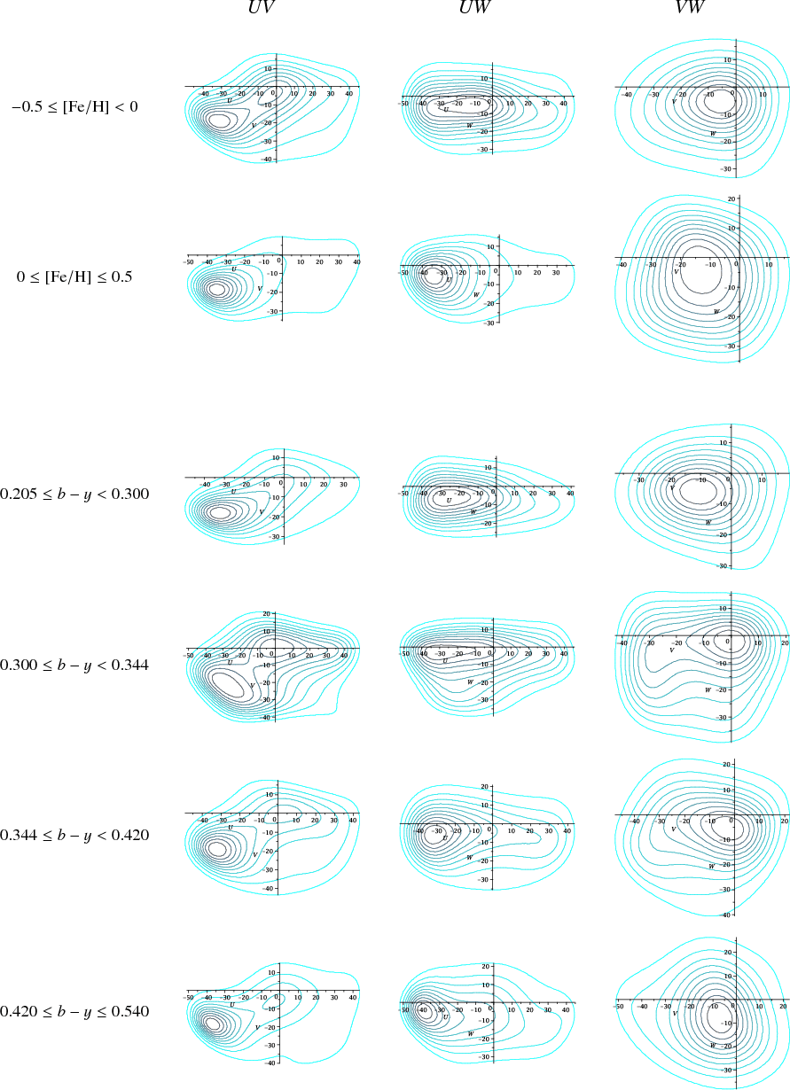
|
Figure 6:
Contour plots of the velocity distribution for stars from the GCS catalogue with
|
| Open with DEXTER | |
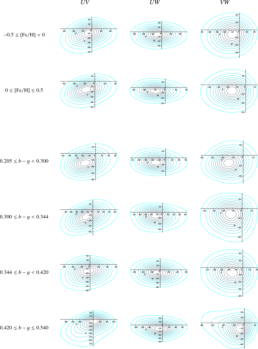
|
Figure 7: Contour plots of the velocity distribution for stars from the total GCS catalogue, obtained from the entropy approach with n=6, in terms of metallicity and colour. |
| Open with DEXTER | |
![\begin{figure}
\par\includegraphics[width=18cm,clip]{12836fg08n.eps}
\end{figure}](/articles/aa/full_html/2010/02/aa12836-09/img144.png)
|
Figure 8:
Series of contour plots and distributions on the UV plane for GCS subsamples selected from
|
| Open with DEXTER | |
3.2 Smaller scale
It is however possible to obtain a more detailed shape for the velocity
distribution for specific subsamples, allowing comparison of the
results of our approach with the small-scale structure sustained by
moving groups as described by other authors. By selecting samples
with bounded peculiar velocity, such as
![]() km s-1 (256 stars), 10 km s-1 (498 stars), or 20 km s-1 (2817 stars), a more complex structure is manifest on the UV plane,
but also in the vertical direction. The shape of the distribution
becomes softer while increasing the size of the sample. Because of
this, the substructure of thin disc subsamples with less stars become
statistical fluctuations within larger subsamples, up to describing a
sufficiently complete distribution of the thin disc. Thus the clue is
to find a clean and representative thin disc sample. The cut
km s-1 (256 stars), 10 km s-1 (498 stars), or 20 km s-1 (2817 stars), a more complex structure is manifest on the UV plane,
but also in the vertical direction. The shape of the distribution
becomes softer while increasing the size of the sample. Because of
this, the substructure of thin disc subsamples with less stars become
statistical fluctuations within larger subsamples, up to describing a
sufficiently complete distribution of the thin disc. Thus the clue is
to find a clean and representative thin disc sample. The cut
![]() km s-1
therefore seems to be a good value that includes most of thin disc
stars and excludes thick disc stars, but it is still far from
being a complete thin disc sample. Samples selected from small peculiar
velocities have some limitations. On one hand, they contain few stars,
so that their distribution may not be bell-shaped enough.
Furthermore, their moments have greater uncertainties. On the other
hand, the boundary of the distribution is fixed by the velocity limit
of the sample, which may cut down some well-defined structures.
Fortunately, there is a way to avoid this problem.
In Papers I and II, consecutive stellar populations were
merged to nested subsamples in terms of several sampling parameters:
maximum absolute velocity, peculiar velocity, vertical
velocity, etc. Optimal values of these sampling parameters allowed
the segregation of these populations. For the complete GCS sample,
once the stars are classified according to the probability of belonging
to any of the local Galactic components (Paper II), a highly
significative correlation is obtained between the expected population
of a star and its absolute velocity
km s-1
therefore seems to be a good value that includes most of thin disc
stars and excludes thick disc stars, but it is still far from
being a complete thin disc sample. Samples selected from small peculiar
velocities have some limitations. On one hand, they contain few stars,
so that their distribution may not be bell-shaped enough.
Furthermore, their moments have greater uncertainties. On the other
hand, the boundary of the distribution is fixed by the velocity limit
of the sample, which may cut down some well-defined structures.
Fortunately, there is a way to avoid this problem.
In Papers I and II, consecutive stellar populations were
merged to nested subsamples in terms of several sampling parameters:
maximum absolute velocity, peculiar velocity, vertical
velocity, etc. Optimal values of these sampling parameters allowed
the segregation of these populations. For the complete GCS sample,
once the stars are classified according to the probability of belonging
to any of the local Galactic components (Paper II), a highly
significative correlation is obtained between the expected population
of a star and its absolute velocity ![]() .
The expected value is similarly highly correlated with the planar
eccentricity, and also correlated with rotation velocity,
.
The expected value is similarly highly correlated with the planar
eccentricity, and also correlated with rotation velocity,
![]() and
metallicity. The colour is few correlated with the expected population
and the other preceding properties. Therefore significant partial
correlations between couples of the former star properties exist.
However, when the sample is bounded to
and
metallicity. The colour is few correlated with the expected population
and the other preceding properties. Therefore significant partial
correlations between couples of the former star properties exist.
However, when the sample is bounded to
![]() km s-1,
by leaving aside thick disc and halo stars, the only
significant partial correlation that is maintained is the absolute
velocity and the eccentricity, as well as the expected population
with them. That means that the other properties are only relevant for
segregating thick-disc or halo stars, but are not useful within the
very thin disc. As discussed in Paper II, the sampling
parameter is related to the isolating integrals of the star motion.
Both the absolute velocity and the eccentricity satisfy this
requirement. The former is less discriminant, but is a direct
measure from the star. The latter is more discriminant, but requires
computing the orbital parameters, with the need of additional
hypothesis on the potential, symmetries, stationarity, mean motion,
solar position, etc. Therefore, it is possible to use the
eccentricity not for segregating populations, as e.g., Pauli
et al. (2005) or Vidojevic & Ninkovic (2009), but as an improved sampling parameter to select subsamples.
km s-1,
by leaving aside thick disc and halo stars, the only
significant partial correlation that is maintained is the absolute
velocity and the eccentricity, as well as the expected population
with them. That means that the other properties are only relevant for
segregating thick-disc or halo stars, but are not useful within the
very thin disc. As discussed in Paper II, the sampling
parameter is related to the isolating integrals of the star motion.
Both the absolute velocity and the eccentricity satisfy this
requirement. The former is less discriminant, but is a direct
measure from the star. The latter is more discriminant, but requires
computing the orbital parameters, with the need of additional
hypothesis on the potential, symmetries, stationarity, mean motion,
solar position, etc. Therefore, it is possible to use the
eccentricity not for segregating populations, as e.g., Pauli
et al. (2005) or Vidojevic & Ninkovic (2009), but as an improved sampling parameter to select subsamples.
For samples with maximum eccentricities 0.01 (220 stars), 0.02
(591 stars), 0.03 (1058 stars), 0.05 (2465 stars), 0.1
(7095 stars), 0.15 (9545 stars), 0.2
(10 903 stars), and 0.3 (11 826 stars), with the
additional condition
![]() kpc
to avoid contamination from stars not belonging to the thin disc, the
maximum entropy approach provides the series of plots in Fig. 8.
Both previous limitations introduced by the peculiar velocity boundary
have disappeared. For example, the structure described by the plot
kpc
to avoid contamination from stars not belonging to the thin disc, the
maximum entropy approach provides the series of plots in Fig. 8.
Both previous limitations introduced by the peculiar velocity boundary
have disappeared. For example, the structure described by the plot
![]() km s-1
with 498 stars is now more completely described from the plot with
maximum eccentricity 0.05 with 2465 stars. Similarly, the
shape of the distribution is no longer forced by the sampling
parameter. The eccentricity then behaves as a very good sampling
parameter that allows us to distinguish between different eccentricity layers
within the thin disc and enables us to visualise the structure below
each layer. In the lower layers, with maximum eccentricities 0.01
and 0.02, the velocity distribution shows a hole around the local
standard of rest (LSR), taken as (-10., -5.23,
7.17) km s-1 (Dehnen & Binney 1998),
which is the mean of the distribution. Those lowest eccentricity stars
are moving around the LSR and have velocities distributed on a ring
with some peaks around the LSR. The radial velocities are symmetrically
grouped into two main bulks at each side of the LSR. This behaviour is
maintained up to eccentricity e = 0.03, where the LSR hole
begins to be filled by the group of stars corresponding to the Coma
Berenices moving group, nearly at the same LSR velocity.
In addition, three stellar groups around the LSR conform the basic
structure: NGC 1901, a group that can be part of the middle
branch (Skuljan et al. 1999), and a part of the Pleiades group. The structure is the same as described by Bovy et al. (2009) and by previous works of Dehnen (1998), Skuljan et al. (1999), Famaey et al. (2005, 2008), with the greatest peak in NGC 1901.
km s-1
with 498 stars is now more completely described from the plot with
maximum eccentricity 0.05 with 2465 stars. Similarly, the
shape of the distribution is no longer forced by the sampling
parameter. The eccentricity then behaves as a very good sampling
parameter that allows us to distinguish between different eccentricity layers
within the thin disc and enables us to visualise the structure below
each layer. In the lower layers, with maximum eccentricities 0.01
and 0.02, the velocity distribution shows a hole around the local
standard of rest (LSR), taken as (-10., -5.23,
7.17) km s-1 (Dehnen & Binney 1998),
which is the mean of the distribution. Those lowest eccentricity stars
are moving around the LSR and have velocities distributed on a ring
with some peaks around the LSR. The radial velocities are symmetrically
grouped into two main bulks at each side of the LSR. This behaviour is
maintained up to eccentricity e = 0.03, where the LSR hole
begins to be filled by the group of stars corresponding to the Coma
Berenices moving group, nearly at the same LSR velocity.
In addition, three stellar groups around the LSR conform the basic
structure: NGC 1901, a group that can be part of the middle
branch (Skuljan et al. 1999), and a part of the Pleiades group. The structure is the same as described by Bovy et al. (2009) and by previous works of Dehnen (1998), Skuljan et al. (1999), Famaey et al. (2005, 2008), with the greatest peak in NGC 1901.
For e=0.05 the structure is maintained and enlarged.
It incorporates a new group of stars also associated with the
middle branch, which is not referred to as a moving group by Bovy
et al. (2009), but is
the centre of their Gaussian component with the largest weight.
In the range of eccentricities from 0.05 to 0.1, the
small previous structures are diluted in a background distribution, and
only the Pleiades group remains. The main weight of the distribution is
now in the stars around the Hyades group. A stellar group around
the Sirius/UMa stream arises at positive radial velocities. For e=0.15,
that is, approximately the higher eccentricity before appearing
thick disc stars, the distribution is divided into about half:
one bulk with negative radial and rotation mean velocities with
respect to the LSR, which contain the main groups Hyades and Pleiades;
and another one with positive values around Sirius and UMa stream.
For higher eccentricities, the distribution becomes similar to the one
corresponding to the thin disc. In particular, for e=0.3,
with a fraction of 90% of the whole sample, we get a distribution
similar to the thin disc of Paper II (obtained by two different
methods: MEMPHIS algorithm and the method of Galactic orbits), with
dispersions and vertex deviation
![]() = (29.1
= (29.1 ![]() 0.2, 18.1
0.2, 18.1 ![]() 0.1, 11.6
0.1, 11.6 ![]() 0.1;
0.1; ![]()
![]() 1).
1).
Thus, for eccentricities below 0.15, there is a general trend in the
radial direction: the main weight of the distribution is
symmetrically placed around the LSR. Thus, the velocity distribution of
the thin disc is supported by two major stellar groups with opposite
radial velocities around the LSR, with a dearth of stars at the LSR.
One bulk, with positive radial velocity, has a mean velocity similar to
the Sun or slightly higher, with a lower peak but a wider distribution.
The other one, with radial velocity
![]() km s-1, has a mean rotation
km s-1, has a mean rotation
![]() km s-1 and a higher peak. This behaviour is definitively broken for eccentricities
km s-1 and a higher peak. This behaviour is definitively broken for eccentricities
![]() .
.
4 Discussion
The situation described in the preceding section, where the star velocities are distributed for low eccentricities along the U direction
with a local minimum at the LSR velocity, may have a simple
explanation: a mixture of stars with a discrete number of radial
oscillation periods. In the special case of a nearly planar orbit,
where the planar eccentricity is low enough that the amplitude of the
vertical motion becomes independent of the radial motion, the motion of
a star can be studied as a case of epicyclic orbit. Let us
remember that, if a nearly planar orbit is projected onto the
Galactic plane, its distance to the Galactic centre oscillates between
two limiting values ![]() and
and ![]() .
The planar eccentricity e is then defined as
.
The planar eccentricity e is then defined as

which is a dimensionless measure of the deviation from the circular motion in the plane of symmetry.
The orbits in the Galactic disc are nearly planar, and their planar
eccentricities may be significantly different from zero (Vidojevic
& Ninkovic 2009).
Thus, the epicyclic approximation can be used for the current disc
sample (Paper II). It is commonly assumed that moving groups
of young stars are born in nearly circular orbits (e.g. Dehnen 1998)
and, with age, they are transformed into more eccentric orbits, which
oscillate locally around the LSR (assumed to be in circular motion,
![]() ,
for steady state and axisymmetric systems). Thus, the radial
velocity of a star oscillating around the LSR with a period T may be written as
,
for steady state and axisymmetric systems). Thus, the radial
velocity of a star oscillating around the LSR with a period T may be written as

where the amplitude is proportional to the eccentricity,
For a sufficiently great t, e.g., taking several periods, we may also assume that t is uniformly distributed within the interval [0,1], so that its probability density function is ft(t)=1,
![]() ,
and zero otherwise. We may ask for the distribution of U around the LSR velocity, that is, for the probability of finding a star velocity at any given value within [-a,a]. Since
,
and zero otherwise. We may ask for the distribution of U around the LSR velocity, that is, for the probability of finding a star velocity at any given value within [-a,a]. Since
![]() ,
and this is a two-valued function, the probability density function fU(U;a), for a given amplitude a, is easily obtained as
2 ft(t) |t'(U)|. Thus,
,
and this is a two-valued function, the probability density function fU(U;a), for a given amplitude a, is easily obtained as
2 ft(t) |t'(U)|. Thus,
![\begin{displaymath}%
f_U(U;a)= \frac{1}{\pi} \frac{1}{\sqrt{a^2-U^2}},\quad U\in [-a,a],
\end{displaymath}](/articles/aa/full_html/2010/02/aa12836-09/img160.png)
and zero out of this interval. As seen in Fig. 21b, for an arbitrary value a=1, it is less probable to find the star with nearly zero velocity, which means near the extreme positions
We may think of a mixture of stars with the same oscillation period and
different eccentricities, from zero eccentricity and amplitude, a=0, up to greater amplitudes, say a=A. Let us assume a normalised density function ![]() of stars in terms of the amplitude a. Then the cumulative density function hU(U;A) is obtained by integration over a as
of stars in terms of the amplitude a. Then the cumulative density function hU(U;A) is obtained by integration over a as
![\begin{figure}
\par\includegraphics[width=6.5cm,clip]{12836fg80.eps}
\end{figure}](/articles/aa/full_html/2010/02/aa12836-09/img163.png)
|
Figure 9:
Distribution of eccentricities for the GCS sample. The probability
density function obtained from the histogram is approximately
lognormal. In the x-axis, the interval [0,1] of eccentricities is divided into 50 bins. The variable x=50 e is lognormal with m=1.75 and
|
| Open with DEXTER | |
Depending on how the stars are distributed in terms of the amplitude,
we may get different symmetric distributions around the LSR. For a
fixed period T,
this depends on the distribution of eccentricity. The distribution of
eccentricity is approximately lognormal, similar to the distribution of
wealth in a country, as shown in Fig. 9
from the histogram for the GCS sample, where the
interval [0,1] of eccentricities is divided into 50 bins on
the x-axis (x=50 e is approximately lognormal with m=1.75 and
![]() ).
).
To find out the shape of hU(U;A)
for a group of stars with the same period, several simulations are
carried out for arbitrary values of the amplitude, by assuming ![]() lognormal.
Bimodal distributions around the origin (LSR) are always obtained, like
the plots (c), (d), and (e) of
Fig. 10. The mathematical
reason is that the lognormal distribution vanishes in a
neighbourhood of zero. (It is tangent to zero at the origin.)
However, the wider the distribution wing, the less significant the
bimodality, since the behaviour for low amplitudes becomes a smaller
structure when larger amplitudes are considered. The distribution tends
to be Gaussian. In the case of a discrete mixture of stars with
different periods, we should get a mixture of densities hU(U;A)
with similar properties, which could explain the radial velocity shape
obtained for the inner thin disc. However, for a continuous
mixture of populations in terms of oscillation periods, the bimodal
structure may be irrelevant. For example, apart from statistical
fluctuations, as increasing T, the density function
lognormal.
Bimodal distributions around the origin (LSR) are always obtained, like
the plots (c), (d), and (e) of
Fig. 10. The mathematical
reason is that the lognormal distribution vanishes in a
neighbourhood of zero. (It is tangent to zero at the origin.)
However, the wider the distribution wing, the less significant the
bimodality, since the behaviour for low amplitudes becomes a smaller
structure when larger amplitudes are considered. The distribution tends
to be Gaussian. In the case of a discrete mixture of stars with
different periods, we should get a mixture of densities hU(U;A)
with similar properties, which could explain the radial velocity shape
obtained for the inner thin disc. However, for a continuous
mixture of populations in terms of oscillation periods, the bimodal
structure may be irrelevant. For example, apart from statistical
fluctuations, as increasing T, the density function ![]() may become more populated around zero, so that it is no longer
tangent to zero at the origin of amplitudes. Then,
a high-peaked hU(U;A) may be obtained at the origin, for low values of A. In general, if in a neighbourhood of the origin,
may become more populated around zero, so that it is no longer
tangent to zero at the origin of amplitudes. Then,
a high-peaked hU(U;A) may be obtained at the origin, for low values of A. In general, if in a neighbourhood of the origin, ![]() behaves as ap, with
behaves as ap, with
![]() we then get smooth unimodal distributions centred at the origin. On the
other hand, it is easy to prove that, if the radial velocity
does not oscillate symmetrically around the LSR meaning a slight
deviation from the epicyclic approximation, the peaks of hU(U;A)
become non-symmetric around the LSR. Therefore, these simple
simulations reproduce the actual situation for low eccentricities
approximately.
we then get smooth unimodal distributions centred at the origin. On the
other hand, it is easy to prove that, if the radial velocity
does not oscillate symmetrically around the LSR meaning a slight
deviation from the epicyclic approximation, the peaks of hU(U;A)
become non-symmetric around the LSR. Therefore, these simple
simulations reproduce the actual situation for low eccentricities
approximately.
As a result, the thin disc contain two major streams moving with opposite radial directions around the LSR, one with small positive radial mean velocity and rotation similar to the Sun, and the other with negative radial mean velocity and lower rotation. For each subsystem, we could assume some less restrictive hypotheses, such as point-axial symmetry (opposite points through an axis, allowing, in particular, spiral structures) or a time-dependent model, in order to describe the non-vanishing radial velocity of their centroids and the vertex deviation of their approximate velocity ellipsoids. Thus, a general Chandrasekhar point-axial model (Sanz-Subirana & Català-Poch 1987; Juan-Zornoza et al. 1990, 1995) should be the simplest approximation, where, despite the non-cylindrical symmetry of the system, the solution of Chandrasekhar's equations system yields an axisymmetric potential. In this case, it is interesting to recall the relationship between the vertex deviation and the radial mean velocity.
| Figure 10: Simulated distribution
of radial velocities for arbitrary values of the amplitude,
by assuming the epicyclic approximation and |
|
| Open with DEXTER | |
| Figure 11:
( Left) Velocity ellipsoids, in blue, depicted according to Eqs. (23) and (24), from total moments corresponding to the sample with eccentricities |
|
| Open with DEXTER | |
It is well known that the vertex deviation ![]() of a velocity ellipsoid depends on the second central moments in the form
of a velocity ellipsoid depends on the second central moments in the form
|
(22) |
Thus, if
where U0 is the radial mean velocity,
Thus, according to Eq. (23), a velocity ellipsoid with a positive [negative] vertex deviation might be associated with a loss of axisymmetry and with a radial motion towards [against] the Galactic centre.
In Fig. 11 (left) the
two major stellar groups with opposite radial velocities around the
LSR, which support the largest structure within the thin disc, are
associated with two velocity ellipsoids with similar total dispersions.
The one moving toward the Galactic centre, with radial and rotation
galactocentric mean velocities
![]() ,
and the other one, toward the anticentre, with mean motion U0=-15,
,
and the other one, toward the anticentre, with mean motion U0=-15,
![]() .
The LSR is placed in the middle of both ellipsoids in a similar
situation to the sample with maximum eccentricity 0.15.
By assuming the same mixture proportions n'=n'', the partial diagonal central moments
.
The LSR is placed in the middle of both ellipsoids in a similar
situation to the sample with maximum eccentricity 0.15.
By assuming the same mixture proportions n'=n'', the partial diagonal central moments
![]() are obtained from totals and from their deferential mean velocity
u'i-u''i, from the usual relationship
are obtained from totals and from their deferential mean velocity
u'i-u''i, from the usual relationship
The vertex deviation of each ellipsoid is obtained from Eq. (23). The total moments are taken from the sample with maximum eccentricity e=0.3. The graph shows the partial ellipsoids
5 Conclusions
Although successfully applied to a wide disparity of actual problems, the maximum entropy approach has rarely been used to solve the classical moment problem of stellar kinematics. Instead, a number of statistical techniques, maximum likelihood-based multivariate sampling algorithms, wavelet-based algorithms, among others, up to the present date had been proved to be more appropriate than the moment method for accurately describing the local stellar velocity distribution. The moment approach had two basic difficulties compared to other methods: the low accuracy of available data and the complexity of the trivariate model for estimating the parameters. Nowadays, with larger and more precise stellar catalogues, it is possible to compute a reasonable number of moments with sufficient accuracy. On the other hand, the parameter estimation for a maximum entropy function requires some complex computational procedures when working from the minimum set of moment constraints. In contrast, if an extended set of moments is used, the current method provides a linear estimation algorithm, so that a Gramian system of equations leads to a fast and suitable estimation of the smoothest velocity distribution that is consistent with the available constraints. It therefore tends to smooth all the statistical fluctuations of the sample out, so that it is more appropriate to study the velocity distribution of large stellar samples, instead of particular moving groups. The estimation method is, however, specific to bell-shaped distributions.
The resulting features of the local velocity distribution are
similar for the complete HIPPARCOS Sample I and GCS
Sample II, although, as expected, the latter provides more
accurate results due to the lower uncertainties of radial velocity
measurements. The whole distribution shows a nearly constant vertex
deviation in the pseudo ellipsoidal level curves, as well as a
nearly constant axis ratio. According to the most significant
polynomial coefficients, the resulting density function can be
expressed as the product of two exponential functions in the form of
Eq. (17). The background ellipsoidal shape has axis ratios 1:0.7:0.5 and a symmetry plane W=0. The overall vertex deviation in the UV velocity components is approximately
![]() .
Some characteristic parameters of the distribution are summarised in Table 3. The function
.
Some characteristic parameters of the distribution are summarised in Table 3. The function
![]() may be interpreted as a perturbation factor, and is even and at least quadratic in the V velocity
alone. It accounts for the skewness and the shift in the velocity
ellipsoids in terms of the rotation velocity. This is clearly visible
on the UV and VW planes of Fig. 1,
and may be interpreted with regard to the heating of disc stars, which
is also correlated with a decreasing galactocentric rotation velocity,
as expected from Strömberg's law. The resulting overall
distribution has zero curtosis in the W velocity, and,
within
may be interpreted as a perturbation factor, and is even and at least quadratic in the V velocity
alone. It accounts for the skewness and the shift in the velocity
ellipsoids in terms of the rotation velocity. This is clearly visible
on the UV and VW planes of Fig. 1,
and may be interpreted with regard to the heating of disc stars, which
is also correlated with a decreasing galactocentric rotation velocity,
as expected from Strömberg's law. The resulting overall
distribution has zero curtosis in the W velocity, and,
within ![]() level, in the U component for the more accurate GCS sample.
level, in the U component for the more accurate GCS sample.
On the other hand, the entropy method offers an excellent estimation of
the truncated velocity distributions of Samples III and IV,
which only contain thin disc stars. For these subsamples,
a Gaussian mixture approach was impossible in Paper I. This
method can therefore be used as an alternative way to study multimodal
distributions. For star velocities
![]() km s-1,
the tentative mixture (with a very large chi-squared fitting
error) obtained in Paper I suggested a superposition of two
enlarged pseudo-ellipsoidal distributions, mainly along the radial
direction, with very overlapped wings, and a separation of 28
km s-1,
the tentative mixture (with a very large chi-squared fitting
error) obtained in Paper I suggested a superposition of two
enlarged pseudo-ellipsoidal distributions, mainly along the radial
direction, with very overlapped wings, and a separation of 28 ![]() 9 km s-1
between means. For Sample IV, the separation of the two peaks
(the ``U-anomaly'') along the radial direction may now be
straightforwardly estimated in 30-35 km s-1 from the contour plots obtained from the moment constraints. Figures 2 and 3 show a strongly asymmetric velocity dispersion on the plane UV, and nearly laminar isocontours of the W velocity component along the radial direction. There is a large radial velocity dispersion on the UV plane,
in the direction of the gravitational gradient, and a very small
dispersion in the direction perpendicular to the galactic plane. On the
VW plane, the isotropy is slightly recovered. However,
the higher resolution contour plots obtained from Sample IV allow
more detailed analysis. A first look at the UW plane of Fig. 3 (n=6)
shows a core distribution with negative radial peculiar velocity, while
there is a clear unimodal behaviour with positive peculiar rotation
velocity on the VW plane. However, those high-density regions of the distribution are not simultaneous on the UV plane, but are associated with different large stellar groups.
9 km s-1
between means. For Sample IV, the separation of the two peaks
(the ``U-anomaly'') along the radial direction may now be
straightforwardly estimated in 30-35 km s-1 from the contour plots obtained from the moment constraints. Figures 2 and 3 show a strongly asymmetric velocity dispersion on the plane UV, and nearly laminar isocontours of the W velocity component along the radial direction. There is a large radial velocity dispersion on the UV plane,
in the direction of the gravitational gradient, and a very small
dispersion in the direction perpendicular to the galactic plane. On the
VW plane, the isotropy is slightly recovered. However,
the higher resolution contour plots obtained from Sample IV allow
more detailed analysis. A first look at the UW plane of Fig. 3 (n=6)
shows a core distribution with negative radial peculiar velocity, while
there is a clear unimodal behaviour with positive peculiar rotation
velocity on the VW plane. However, those high-density regions of the distribution are not simultaneous on the UV plane, but are associated with different large stellar groups.
In addition to limited velocity distributions, other truncated
distributions were analysed in terms of metallicity, colour, maximum
distance to the Galactic plane, and eccentricity. Those star properties
were correlated with the star's expected population obtained in
Paper II. The only significant correlations that are maintained
within thin disc stars are the absolute velocity and the eccentricity,
since metallicity and
![]() are
more appropriate for segregating
thick disc and halo stars from the thin disc. In particular, the
eccentricity, which is directly related to the isolating integrals of
the star motion, is more discriminating than the absolute velocity
for selecting subsamples. However, a part of thin and thick disc
stars may have similar eccentricities. Then, to isolate thin disc
stars, it is necessary to combine two sampling parameters:
eccentricity and
are
more appropriate for segregating
thick disc and halo stars from the thin disc. In particular, the
eccentricity, which is directly related to the isolating integrals of
the star motion, is more discriminating than the absolute velocity
for selecting subsamples. However, a part of thin and thick disc
stars may have similar eccentricities. Then, to isolate thin disc
stars, it is necessary to combine two sampling parameters:
eccentricity and
![]() .
A representative thin disc, containing 90% of the whole
sample, is selected from maximum eccentricity 0.3 and
.
A representative thin disc, containing 90% of the whole
sample, is selected from maximum eccentricity 0.3 and
![]() kpc.
Its central moments are similar to the ones obtained for the thin
disc in Paper II. Furthermore, within the thin disc sample, the
eccentricity behaves as an excellent sampling parameter that
distinguishes between different eccentricity layers allowing subjacent
structures to be visualised.
kpc.
Its central moments are similar to the ones obtained for the thin
disc in Paper II. Furthermore, within the thin disc sample, the
eccentricity behaves as an excellent sampling parameter that
distinguishes between different eccentricity layers allowing subjacent
structures to be visualised.
For subsamples obtained from eccentricities e<0.15,
the maximum entropy method is able to plot
the classical moving groups composing the small-scale structure of the
velocity distribution, as described from other algorithms based on
an arbitrary number of mixture components, wavelet transforms, or
maximum likelihood (e.g., Famaey et al. 2008; Veltz
et al. 2008; Skuljan et al. 1999; Dehnen 1998), especially those providing a modest amount of complexity (Bovy et al. 2009).
For these subsamples with small eccentricities, there is a general
trend: the star velocities are approximately symmetrically distributed
around the LSR in the radial direction. In most cases the
distribution is bimodal, with a dearth of stars at the LSR. At the
end, for e=0.15,
the core distribution of the thin disc is supported by two major
stellar groups with opposite radial velocities, referred to
the LSR. One bulk, with zero or small positive heliocentric
radial mean velocity, has a lower peak but a wider distribution around
Sirius/UMa stream. The other one, with radial velocity about
-30 km s-1, has mean rotation
![]() km s-1 and a higher peak, containing the main groups Hyades and Pleiades.
km s-1 and a higher peak, containing the main groups Hyades and Pleiades.
For stars with a similar period of oscillation around the LSR in the
radial direction (under the epicyclic approximation), several
simulations allow us to confirm that such a two-peaked distribution of
radial velocities is due to a lognormal distribution of the
eccentricities. For a mixture of stars with different periods and
a lognormal distribution of the velocity amplitude of the stellar
orbits, the bimodal shape is maintained. However, if the number of
stars with nearly vanishing amplitude increases, then the radial
velocity distribution becomes unimodal, similar to the total thin disc
sample with ![]() .
.
The bimodal behaviour of the central disc associated with the previous major subsystems may then be explained from two different phenomena. On one hand, it may be a perturbation similar to a pressure wave acting in part along the radial direction that induces an oscillation of the radial velocity around the LSR. Let us remember that the oscillation of each subsystem centroid along the U direction is also the expected motion of axisymmetric systems under steady state potentials (e.g. Cubarsi et al. 1990). On the other hand, both kinematical major groups, which actually are placed at the solar position, are in opposite oscillation states. In addition both groups have a difference of about 20 km s-1 in rotation mean velocity, so that one group of stars actually surpasses the other group. Therefore, the apparent vertex deviation of the thin disc may stem from the swinging of those major kinematic groups. A scenario of a continuously changing orientation of the disc pseudo ellipsoid is then possible.
Appendix A
We need to write
![]() in Eq. (15)
by using a slightly different notation, with Latin indices instead of
Greek indices, so that each term accounts for products of the same
degree in the velocities. Thus, by using hereafter Einstein's summation
criterion for repeated indices, we may write
in Eq. (15)
by using a slightly different notation, with Latin indices instead of
Greek indices, so that each term accounts for products of the same
degree in the velocities. Thus, by using hereafter Einstein's summation
criterion for repeated indices, we may write
In the summation term corresponding to the
which establishes the correspondence between the Greek and Latin index notations for the coefficients of
When
![]() ,
Eq. (15)
converges to the true distribution. Then, if the velocity
distribution is expressed as a power series of the velocities,
we have
,
Eq. (15)
converges to the true distribution. Then, if the velocity
distribution is expressed as a power series of the velocities,
we have
which is a similar relationship between generalised moments
A maximum entropy distribution function can exhibit several modes. In the trivariate case, if Eq. (15) is a polynomial of even degree n, the distribution can exhibit (n/2)3 modes, since an univariate exponential with a polynomial of degree n may have up to n/2 modes. In general, it is necessary to estimate less number of parameters for Eq. (15) than for a mixture of trivariate Gaussian distributions accounting for the same number of modes.
A.1. Boundary conditions
We now study a quite general case for fitting a defined set of velocity moments, up to order 2(n-1), with a maximum entropy velocity distribution containing a polynomial of degree n, which allows a simple and linear estimation of the polynomial coefficients. By using Latin indices notation for
![]() ,
according to Eq. (25), we assume that all the moments in Eq. (2)
exist, which is equivalent to considering the distribution function to
be a square-integrable function in the velocity domain
,
according to Eq. (25), we assume that all the moments in Eq. (2)
exist, which is equivalent to considering the distribution function to
be a square-integrable function in the velocity domain ![]() .
The scalar
.
The scalar ![]() is the normalisation factor, and, in general, all of the above coefficients are symmetric elements of k-rank tensors
is the normalisation factor, and, in general, all of the above coefficients are symmetric elements of k-rank tensors
![]() ;
;
![]() involved in Eq. (25).
involved in Eq. (25).
The other coefficients than ![]() can be obtained by using the property
can be obtained by using the property
![\begin{displaymath}%
\int_{\Gamma_V} \nabla_{\vec{V}} \left[(\vec{V})^m {\rm e}^{{\cal P}_n}\right] {\rm d}^3\vec{V}=(0)^{n+1},
\end{displaymath}](/articles/aa/full_html/2010/02/aa12836-09/img201.png)
which is a direct consequence of Eq. (11) and, in particular, is fulfilled by any solution of the moment equations.
The above integral is an (n+1)-rank tensor, which is symmetric with respect to the indices of the tensor power
![]() .
Thus, when integrating Eq. (28) by components and the conditions of Eq. (11) are applied over the domain of any variable
Vim+1, we get
.
Thus, when integrating Eq. (28) by components and the conditions of Eq. (11) are applied over the domain of any variable
Vim+1, we get
In the case of a finite velocity domain, if the density function is bell-shaped, the null value of the righthand side might be substituted by a tolerance error, namely
such that this value can be neglected on condition of being significantly small
In particular, for m=0, since

we have
Similarly, for m=1,
where
And, in general, for ![]() ,
we get
,
we get
where the hat indicates the omitted factors. Once more, bearing Eq. (31) in mind, the identity Eq. (28) yields
Since the first integral is symmetric with respect to permutation of indices, and in general it is not null, then the second integral
must be symmetric, too. Indeed, Eqs. (35) and (36) are equivalent to those obtained in Cubarsi (2007) as Eqs. (22) and (29), which were derived for expressing the conservation of pressures.
In this new context, the above identities will provide a linear method of fitting any desired set of moments. In contrast to the usual maximum entropy methods for the moments problem, which are nonlinear and not well conditioned enough, the present method allows all of the coefficients to be determined with accuracy.
First we evaluate
![]() starting from Eq. (25),
starting from Eq. (25),
To obtain all of the elements of tensors
which stands for a set of 3 scalar equations, k=1,2,3. For m=1, also by taking Eqs. (33) and (37) into account, we get
Hence, this set of relations, for i,k=1,2,3, thanks to the symmetry of Eq. (36), provides 6 independent scalar equations.
Table A.1:
Matrix ![]() is a symmetric matrix of inner products of the velocity components
is a symmetric matrix of inner products of the velocity components
![]() ,
according to Latin indices, with
,
according to Latin indices, with
![]() and the other indices sorted as
and the other indices sorted as
![]() and
and
![]()
![]() .
.
Table A.2: The system of Eqs. (42) grouped as a three column matrix, on their righthand side.
And, in general, for m=n-1, from Eq. (35) we likewise get
which consists in a set of
Table A.3:
Coefficient submatrix relating the first column ![]() of matrix
of matrix ![]() and the first column
and the first column ![]() of matrix
of matrix ![]() .
.
Finally, the scalar ![]() left to be evaluated may be obtained as the normalisation factor to satisfy
left to be evaluated may be obtained as the normalisation factor to satisfy
Table A.4:
Coefficient submatrix relating the second column ![]() of matrix
of matrix ![]() and the first column
and the first column ![]() of matrix
of matrix ![]() .
.
Table A.5:
Coefficient submatrix relating the third column ![]() of matrix
of matrix ![]() and the third column
and the third column ![]() of matrix
of matrix ![]() .
.
A.2. Gramian system
The three scalar equations involved in Eq. (38), corresponding to m=0, for k=1,2,3, are homogeneous in the elements of tensors
![]() .
In Eq. (39), for m=1, we group the terms containing the elements of
.
In Eq. (39), for m=1, we group the terms containing the elements of
![]() ,
by writing the other ones on the righthand side, and likewise for the general equation with m=n-1, Eq. (40). Thus we obtain the following linear system of equations for the elements of tensors
,
by writing the other ones on the righthand side, and likewise for the general equation with m=n-1, Eq. (40). Thus we obtain the following linear system of equations for the elements of tensors
![]() ,
,
Such a system of equations can be grouped according to three different vectors on its righthand side, for k=1,2,3 in the first two equations and for in=1,2,3 in the general expression. A similar procedure can be applied to the
The system matrix, ![]() shown in Table A.1, can be interpreted as a symmetric matrix of inner products with respect to the weight
shown in Table A.1, can be interpreted as a symmetric matrix of inner products with respect to the weight
![]() of the velocity components
of the velocity components
![]() according to the Latin indices notation, with
according to the Latin indices notation, with
![]() and the other indices sorted as
and the other indices sorted as
![]() and
and
![]() .
Therefore,
.
Therefore, ![]() is
a Gram matrix, symmetric, positive-definite and, among other
well-known properties, it is invertible, meaning the system has a
unique solution. Thus, we may define, according to Table A.2, the following three column matrices
is
a Gram matrix, symmetric, positive-definite and, among other
well-known properties, it is invertible, meaning the system has a
unique solution. Thus, we may define, according to Table A.2, the following three column matrices
![]() and
and
![]() so that the following equality is satisfied:
so that the following equality is satisfied:
This is the numerical form of the system of equations Eq. (42), ready to be solved.
The coefficients to compute are elements of the symmetric tensors
![]() ,
for orders
,
for orders
![]() ,
since the zero order coefficient is the normalisation factor. In total there are
,
since the zero order coefficient is the normalisation factor. In total there are
![]() independent coefficients. Each column of the matrix
independent coefficients. Each column of the matrix ![]() is composed of:
is composed of:
- one element of the symmetric tensor
 ,
which multiplies the moments of orders
,
which multiplies the moments of orders
 in the first column of matrix
  ;
;
- three elements of
 ,
which multiply the moments of orders
,
which multiply the moments of orders
 in the next three columns of matrix ;
- and, in general,
 elements of the symmetric tensor
 ,
which multiply the moments of orders
,
which multiply the moments of orders
 ,
up to the value k=n-1.
,
up to the value k=n-1.
On the other hand, since the matrices ![]() and
and ![]() consist of three column vectors, we dispose of a number of
consist of three column vectors, we dispose of a number of
![]() equations. This number, for n>1,
is always greater than the number of independent unknowns (leaving
out the normalisation factor). For example, in the case n=2, we have 12 equations and 9 independent unknowns, because the symmetric coefficients
equations. This number, for n>1,
is always greater than the number of independent unknowns (leaving
out the normalisation factor). For example, in the case n=2, we have 12 equations and 9 independent unknowns, because the symmetric coefficients
![]() ,
,
![]() ,
and
,
and
![]() are equivalent to
are equivalent to
![]() ,
,
![]() ,
and
,
and
![]() ,
respectively, and similarly for higher values of n.
In general, if the true distribution is indeed a maximum
entropy distribution, the actual moments will be consistent with the
symmetry of the coefficients, but a significant deviation from the
maximum entropy property will produce some non-symmetric coefficients
,
respectively, and similarly for higher values of n.
In general, if the true distribution is indeed a maximum
entropy distribution, the actual moments will be consistent with the
symmetry of the coefficients, but a significant deviation from the
maximum entropy property will produce some non-symmetric coefficients![]() .
To avoid this situation, an equivalent overdeterminate system of
equations is built up, as explained in the next section, where the
symmetric coefficients of tensors
.
To avoid this situation, an equivalent overdeterminate system of
equations is built up, as explained in the next section, where the
symmetric coefficients of tensors
![]() will
not be repeated in the vector of unknowns. The system is solved by
applying a least squares method, so that to get the minimum
squared error of the fit, it is weighted in terms of the inverse
sampling variances
will
not be repeated in the vector of unknowns. The system is solved by
applying a least squares method, so that to get the minimum
squared error of the fit, it is weighted in terms of the inverse
sampling variances
![]() of the moments up to order n-2, in the righthand side of Eq. (42).
In addition, a predictor-corrector method is applied to
evaluate the variance matrix of the unknowns, as detailed below.
of the moments up to order n-2, in the righthand side of Eq. (42).
In addition, a predictor-corrector method is applied to
evaluate the variance matrix of the unknowns, as detailed below.
A.3. Parameter estimation
The overdeterminate system of equations, which is equivalent to Eq. (43), is written as
| (44) |
where the only unknowns are the non-identical elements of the symmetric tensors
The first column ![]() (Table A.2) of matrix
(Table A.2) of matrix ![]() and the first column
and the first column ![]() of matrix
of matrix ![]() are related by the coefficient submatrix of Table A.3. The second column
are related by the coefficient submatrix of Table A.3. The second column ![]() of matrix
of matrix ![]() and the first column
and the first column ![]() of matrix
of matrix ![]() are related by the coefficient submatrix of Table A.4. The third column
are related by the coefficient submatrix of Table A.4. The third column ![]() of matrix
of matrix ![]() and the third column
and the third column ![]() of matrix
of matrix ![]() are related by the coefficient submatrix of Table A.5.
are related by the coefficient submatrix of Table A.5.
The resulting ![]() matrix is obtained by stacking the three foregoing submatrices. Vector
matrix is obtained by stacking the three foregoing submatrices. Vector ![]() now takes the form
now takes the form

|
||

|
(45) |
The factors multiplying the elements of tensors
It is well known that, if ![]() is the variance matrix for vector
is the variance matrix for vector ![]() ,
which is taken as the diagonal matrix of its sampling variances
,
which is taken as the diagonal matrix of its sampling variances
![]() ,
then the least squares system weighted by
,
then the least squares system weighted by
![]() provides minimum variance estimates for
provides minimum variance estimates for ![]() according to (e.g. Stuart & Ord 1987)
according to (e.g. Stuart & Ord 1987)
|
(46) |
The minimum fitting error is then obtained from the weighted norm of the difference between the observed values and their theoretical predictions,
|
(47) |
The error on the results of the least squares fit, that is the variance
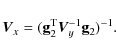
|
(48) |
Some aspects of the fitting procedure must be pointed out:
- (1)
- Some elements of vector
 are exact values, -1 or 0 (left part of Table A.2), thus they have no associated error. However, an initial tolerance error may be assumed for vector ,
which can be associated with the finite domain beyond which the density
function is negligible, as pointed out in Eq. (30). This tolerance error is assumed to be constant and significantly small for all the components (e.g. 10-6), and it is added to the sampling error
are exact values, -1 or 0 (left part of Table A.2), thus they have no associated error. However, an initial tolerance error may be assumed for vector ,
which can be associated with the finite domain beyond which the density
function is negligible, as pointed out in Eq. (30). This tolerance error is assumed to be constant and significantly small for all the components (e.g. 10-6), and it is added to the sampling error
 of the data. The final norm of the quadratic error is computed as
 .
.
- (2)
- In the least squares method, it is generally assumed that the elements of matrix
 are evaluated from exact values, and does not contribute to the error
of the estimates, although it is not true in the current case.
To evaluate the part of the total fitting error due to the
elements of matrix ,
an iterative procedure is started by assuming equal uncertainties for all equations, which are normalised to constant norm f0. Let us call its predicted quadratic error
are evaluated from exact values, and does not contribute to the error
of the estimates, although it is not true in the current case.
To evaluate the part of the total fitting error due to the
elements of matrix ,
an iterative procedure is started by assuming equal uncertainties for all equations, which are normalised to constant norm f0. Let us call its predicted quadratic error
 .
.
- (3)
- By starting from the predicted quadratic error, successive evaluations of the variance matrix
 from the error propagation formula

(49)
are carried out, so that we obtain a corrected quadratic error ,
which is used as a new predicted error, by normalising it to a constant norm f0.
,
which is used as a new predicted error, by normalising it to a constant norm f0.
- (4)
- The algorithm is stopped when a fixed point
 is reached, that is, when
and
have the same direction. It is found that the final quadratic error
of the iterative process does not depend on the initial predicted error, so that the final variance matrix
is the result of a redistribution of weights provided by the matrix
of the least squares system.
is reached, that is, when
and
have the same direction. It is found that the final quadratic error
of the iterative process does not depend on the initial predicted error, so that the final variance matrix
is the result of a redistribution of weights provided by the matrix
of the least squares system.
- (5)
- To compute the final fitting error
 ,
a total sampling variance
,
a total sampling variance
 is assumed as the sum of both independent quadratic errors. The fitting error
is only partially significant, since it is related to the initial value f0, which depends on the initial errors of the data ,
although this way it is possible to compare the goodness of different fittings.
is assumed as the sum of both independent quadratic errors. The fitting error
is only partially significant, since it is related to the initial value f0, which depends on the initial errors of the data ,
although this way it is possible to compare the goodness of different fittings.
Appendix B
The Gramian system and the moment recurrence can be solved straightforwardly for the case n=2,
which corresponds to a Schwarzschild distribution. For the sake of
simplicity, and without losing generality, we use the central
moments
![]() ,
so that
,
so that
![]() .
Then, the Eqs. (38) and (39), for m=0,1, become
.
Then, the Eqs. (38) and (39), for m=0,1, become
and
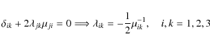
where
Now we can apply the same procedure for ![]() ,
to obtain higher order moments in terms of the second moments. Thus, for m = 2, according to Eq. (40), with m=n-1, and bearing in mind Eq. (50), we have
,
to obtain higher order moments in terms of the second moments. Thus, for m = 2, according to Eq. (40), with m=n-1, and bearing in mind Eq. (50), we have
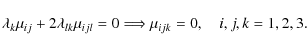
The result accounts for the obvious symmetry of the distribution, with vanishing odd-order central moments.
Similarly, for m = 3, we get
Then, taking into account Eq. (51), we multiply by
The above relationship is the well known property of a Gaussian distribution, which characterises it from having vanishing fourth cumulants.
And, in general, according to Eq. (40), for even m, we obtain a vanishing set of odd-order central moments, and, for odd m, we obtain the relation
Once again, by multiplying by
This is the general relationship of moment recurrence for trivariate normal distributions, which leads to a vanishing set higher-order cumulants. Acknowledgements
The author gratefully acknowledges the comments and suggestions of referees and Editors, in particular, O. Bienaymé, S. Shore, and C. Bertout. The requested deeper analysis of samples and astronomical results has been worthy of an additional effort, by resulting an improved paper and a more convincing usefulness of the method.
References
- Alcobé, S., & Cubarsi, R. 2005, A&A, 442, 929 [NASA ADS] [CrossRef] [EDP Sciences] [Google Scholar]
- Binney, J., & Tremaine, S. 1987, in Galactic Dynamics (Princeton: Princeton University Press) [Google Scholar]
- Binney, J., Dehnen, W., Houk, N., Murray, C. A., & Penston, M. J. 1997, in Hipparcos- Venice'97, ESA SP-402, 473 [Google Scholar]
- Bovy, J., Hogg, D. W., & Roweis, S. T. 2009, ApJ, 700, 1794 [NASA ADS] [CrossRef] [Google Scholar]
- Cercignani, C. 1988, in The Boltzmann Equation and its Applications (Berlin: Springer-Verlag) [Google Scholar]
- Chandrasekhar, S. 1942, in Principles of Stellar Dynamics (New York: Dover Publications Inc.) [Google Scholar]
- Charlier, C. W. L. 1926, in The Motion and the Distribution of the Stars, Berkeley, University of California [Google Scholar]
- Cubarsi, R. 2007, MNRAS, 207, 380 [Google Scholar]
- Cubarsi, R., & Alcobé, S. 2004, A&A, 427, 131 [NASA ADS] [CrossRef] [EDP Sciences] [Google Scholar]
- Cubarsi, R., & Alcobé, S. 2006, A&A, 457, 537 [NASA ADS] [CrossRef] [EDP Sciences] [Google Scholar]
- Cubarsi, R., Sanz, J., & Juan, J. M. 1990, Ap&SS, 170, 197 [NASA ADS] [CrossRef] [Google Scholar]
- Cubarsi, R., Alcobé, S., Vidojevic, S., & Ninkovic, S. 2010, A&A, 510, A102 [NASA ADS] [CrossRef] [EDP Sciences] [Google Scholar]
- de Bruin, R., Salomé, D., & Schaafsma, W. 1999, Comput. Statist. Data Anal., 30, 19 [CrossRef] [Google Scholar]
- Dehnen, W. 1998, AJ, 115, 2384 [NASA ADS] [CrossRef] [Google Scholar]
- Dehnen, W. 1999, AJ, 118, 1201 [NASA ADS] [CrossRef] [Google Scholar]
- Dehnen, W., & Binney, J. J. 1998, MNRAS, 298, 387 [NASA ADS] [CrossRef] [Google Scholar]
- Dejonghe, H. 1983, A&A, 133, 225 [NASA ADS] [Google Scholar]
- Erickson, R. R. 1975, ApJ, 195, 343 [NASA ADS] [CrossRef] [Google Scholar]
- ESA 1992, The Hipparcos Input Catalogue, ESA SP-1136 [Google Scholar]
- ESA 1997, The Hipparcos Catalogue, ESA SP-1200 [Google Scholar]
- Evans, N. W., Haefner, R. M., & de Zeeuw, P. T. 1997, MNRAS, 286, 315 [NASA ADS] [CrossRef] [Google Scholar]
- Famaey, B., Van Caelenberg, K., & Dejonghe, H. 2002, MNRAS, 335, 201 [NASA ADS] [CrossRef] [Google Scholar]
- Famaey, B., Jorissen, A., Luri, X., et al. 2005, A&A, 430, 165 [NASA ADS] [CrossRef] [EDP Sciences] [Google Scholar]
- Famaey, B., Pont, F., Luri, X., et al. 2007, A&A, 461, 957 [NASA ADS] [CrossRef] [EDP Sciences] [Google Scholar]
- Figueras, F., Gomez, A. E., Asiain, R., et al. 1997, in Hipparcos-Venice'97, ed. B. Battrick (Noordwijk: ESA), ESA SP-402, 519 [Google Scholar]
- Fricke, W. 1952, AN, 280, 193 [Google Scholar]
- Gerhard, O. E. 1993, MNRAS, 265, 213 [NASA ADS] [CrossRef] [Google Scholar]
- Gilmore, G., King, I., & Kruit, P.v.d. 1989, in The Milky Way as a Galaxy, ed. R. Buser, & I. King (Geneva: Publ. Geneva Observatory) [Google Scholar]
- Hénon, M. 1973, A&A, 24, 229 [Google Scholar]
- Holmberg, J., Nordström, B., & Andersen, J. 2007, A&A, 475, 519 [NASA ADS] [CrossRef] [EDP Sciences] [MathSciNet] [Google Scholar]
- Jaynes, E. T. 1957a, Phys. Rev., 106, 620 [Google Scholar]
- Jaynes, E. T. 1957b, Phys. Rev., 108, 171 [CrossRef] [MathSciNet] [Google Scholar]
- Jaworsky, W. 1987, J. Phys. A: Math. Gen., 20, 915 [NASA ADS] [CrossRef] [Google Scholar]
- Jiang, Z., & Ossipkov, L. 2007, MNRAS, 379, 1133 [NASA ADS] [CrossRef] [Google Scholar]
- Juan-Zornoza, J. M. 1995, Ph.D. Thesis, Barcelona: Universitat de Barcelona [Google Scholar]
- Juan-Zornoza, J. M., Sanz-Subirana, J., & Cubarsi, R. 1990, Ap&SS, 170, 343 [NASA ADS] [CrossRef] [Google Scholar]
- Kagan, A. M., Linnik, Y. V., & Rao, C. R. 1973, in Characterization Problems in Mathematical Statistics (New York: Wiley) [Google Scholar]
- Kapteyn, J. C. 1922, ApJ, 55, 302 [NASA ADS] [CrossRef] [Google Scholar]
- Kormendy, J., Bender, R., Evans, A. S., & Richstone, D. 1998, AJ, 115, 1823 [NASA ADS] [CrossRef] [Google Scholar]
- Kouskoulas, Y., Pierce, L. E., & Ulaby, F. T. 2004, IEEE Trans. Geosci. Rem. Sens., 42, 457 [NASA ADS] [CrossRef] [Google Scholar]
- Martin, N. F. G., & England, J. W. 1981, in Encyclopaedia of Mathematics and its applications, Mathematical theory of entropy, Reading, Mass (Addison-Wesley), 12 [Google Scholar]
- Mead, L. R., & Papanicolaou, N. 1984, J. Math. Phys., 25, 2405 [Google Scholar]
- Nordström, B., Mayor, M., Andersen, J., et al. 2004, A&A, 418, 989 [NASA ADS] [CrossRef] [EDP Sciences] [Google Scholar]
- Pauli, E.-M., Napiwotzki, R., Heber, U., Altmann, M., & Odenkirchen, M. 2006, A&A, 384, 879 [Google Scholar]
- Sanz-Subirana, J., & Català-Poch, M. A. 1987, in 10th ERAM of the IAU, 4, 267 [Google Scholar]
- Skuljan, J., Hearnshaw, J. B., & Cottrell, P. L. 1999, MNRAS, 308, 731 [NASA ADS] [CrossRef] [Google Scholar]
- Soubiran, C., & Girard, P. 2005, A&A, 438, 139 [NASA ADS] [CrossRef] [EDP Sciences] [Google Scholar]
- Strömberg, G. 1925, ApJ, 61, 363 [NASA ADS] [CrossRef] [Google Scholar]
- Stuart, A., & Ord, J. K. 1987, in Kendall's Advanced Theory of Statistics, Distribution Theory (London: Ch. Griffin & Co.), 1 [Google Scholar]
- Vallenari, A., Pasetto, S., Bertelli, G., et al. 2006, A&A, 451, 125 [NASA ADS] [CrossRef] [EDP Sciences] [Google Scholar]
- van der Marel, R. P., & Franx, M. 1993, ApJ, 407, 525 [NASA ADS] [CrossRef] [Google Scholar]
- Veltz, L., Bienaymé, O., Freeman, K. C., et al. 2008, A&A, 480, 753 [NASA ADS] [CrossRef] [EDP Sciences] [Google Scholar]
- Villani, C. 2002, A review of mathematical topics in collisional kinetic theory, in Handbook of Mathematical Fluid Dynamics, ed. S. Friedlander, & D. Serre (Amsterdam: North-Holland), 1, 71 [Google Scholar]
- Vidojevic, S., & Ninkovic, S. 2009, AN, 330, 46 [NASA ADS] [Google Scholar]
- Vorobyov, E. I., & Theis, Ch. 2008, MNRAS, 383, 817 [NASA ADS] [CrossRef] [Google Scholar]
- White, S. D. M. 1985, ApJ, 294, L99 [NASA ADS] [CrossRef] [Google Scholar]
Footnotes
- ...

![[*]](/icons/foot_motif.png)
- The Stokes operator
 is generally used to simplify
the notation of the Lagrangian derivative
is generally used to simplify
the notation of the Lagrangian derivative
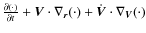 .
.
- ... entropy
- The quotation by Shannon, extracted from Martin & England (1981), is amusing: my greatest concern was how to call it. I thought of calling it ``information''. But the word was overly used, so I decided to call it ``uncertainty''. When I discussed it with John Von Neumann, he had a better idea. He told me: ``you should call it entropy, for two reasons. In the first place your uncertainty has been used in statistical mechanics under that name, so it already has a name. In the second place, and more important, no one knows what entropy really is, so in a debate you will always have the advantage''.
- ...distribution
- When a similar relation holds for the characteristic function
 ,
which is the Fourier transform of density function f, then the coefficients
,
which is the Fourier transform of density function f, then the coefficients
 become proportional to the population moments
 ,
and
,
and
 become proportional to the cumulants of the distribution
 ,
by a factor
,
by a factor
 .
.
- ... small
- For example, the velocity density function f of local stars is approximately Gaussian in the component W perpendicular to the galactic plane, with dispersion
 km s-1. A finite velocity domain
![$I_W=[-W_{\rm max}, W_{\rm max}]$](/articles/aa/full_html/2010/02/aa12836-09/img206.png) could be then assumed, with
could be then assumed, with
 km s-1, where the integral
 is exactly null for even values of n, and remains less than
 for odd values n
< 13. Obviously, the integral is still lower for wider intervals.
Similarly, the local young-disc stars, with absolute heliocentric
velocity up to 51 km s-1, have a velocity dispersion
for odd values n
< 13. Obviously, the integral is still lower for wider intervals.
Similarly, the local young-disc stars, with absolute heliocentric
velocity up to 51 km s-1, have a velocity dispersion
 km s-1. In the similar situation above, we may then assume a finite velocity domain for the truncated velocity distribution with
 km s-1, where such an integral can be neglected up to powers n=12.
- ... coefficients
- This is true for n>2, but for n=2 Appendix B shows that the coefficients
 are related to the second central moments
 ,
which are necessarily symmetric.
,
which are necessarily symmetric.
All Tables
Table 1:
Centred moments
![]() and non-centred moments
and non-centred moments
![]() with their standard errors up to fourth order for the GCS Sample II.
with their standard errors up to fourth order for the GCS Sample II.
Table 2: Centred and non-centred moments with their standard errors up to fourth order for the GCS Sample IV.
Table 3:
Distribution parameters for HIPPARCOS and GCS samples with radial velocity errors up to 2.5 km s-1 (Samples I', II', III', and IV')![]() .
.
Table A.1:
Matrix ![]() is a symmetric matrix of inner products of the velocity components
is a symmetric matrix of inner products of the velocity components
![]() ,
according to Latin indices, with
,
according to Latin indices, with
![]() and the other indices sorted as
and the other indices sorted as
![]() and
and
![]()
![]() .
.
Table A.2: The system of Eqs. (42) grouped as a three column matrix, on their righthand side.
Table A.3:
Coefficient submatrix relating the first column ![]() of matrix
of matrix ![]() and the first column
and the first column ![]() of matrix
of matrix ![]() .
.
Table A.4:
Coefficient submatrix relating the second column ![]() of matrix
of matrix ![]() and the first column
and the first column ![]() of matrix
of matrix ![]() .
.
Table A.5:
Coefficient submatrix relating the third column ![]() of matrix
of matrix ![]() and the third column
and the third column ![]() of matrix
of matrix ![]() .
.
All Figures
|
|
Figure 1:
Contour plots of the local velocity distribution in terms of the
peculiar velocities for HIPPARCOS' Sample I and Sample I'.
The plots are centred on the mean heliocentric velocity
(-10.85, -19.93, -7.49) km s -1 of Sample I', with radial velocity errors up to 2.5 km s-1. The case n=4, by fitting up to sixth moments, leads to more realistic contour plots than a pure ellipsoidal distribution (n=2), although n=6 provides a slightly improvement, by fitting up to tenth moments. The contours indicate levels
|
| Open with DEXTER | |
| In the text | |
|
|
Figure 2:
Contour plots of the velocity distribution for Sample III, from the HIPPARCOS catalogue, for stars with
|
| Open with DEXTER | |
| In the text | |
|
|
Figure 3:
Contour plots of the velocity distribution for Sample IV, from the GCS catalogue, with
|
| Open with DEXTER | |
| In the text | |
|
|
Figure 4: Density functions on the plane UV for the HIPPARCOS Sample III ( left) and the GCS Sample IV ( right). The plots show a bimodal structure around the Hyades stream (highest peak) and the Sirius-UMa stream (lowest peak) for a distribution far from the ellipsoidal hypothesis. |
| Open with DEXTER | |
| In the text | |
|
|
Figure 5:
Distribution of GCS sample stars into populations in terms of absolute
velocity, eccentricity, metallicity, and colour. The blue dots indicate
stars with
|
| Open with DEXTER | |
| In the text | |
|
|
Figure 6:
Contour plots of the velocity distribution for stars from the GCS catalogue with
|
| Open with DEXTER | |
| In the text | |
|
|
Figure 7: Contour plots of the velocity distribution for stars from the total GCS catalogue, obtained from the entropy approach with n=6, in terms of metallicity and colour. |
| Open with DEXTER | |
| In the text | |
|
|
Figure 8:
Series of contour plots and distributions on the UV plane for GCS subsamples selected from
|
| Open with DEXTER | |
| In the text | |
|
|
Figure 9:
Distribution of eccentricities for the GCS sample. The probability
density function obtained from the histogram is approximately
lognormal. In the x-axis, the interval [0,1] of eccentricities is divided into 50 bins. The variable x=50 e is lognormal with m=1.75 and
|
| Open with DEXTER | |
| In the text | |
| |
Figure 10: Simulated distribution
of radial velocities for arbitrary values of the amplitude,
by assuming the epicyclic approximation and |
| Open with DEXTER | |
| In the text | |
| |
Figure 11:
( Left) Velocity ellipsoids, in blue, depicted according to Eqs. (23) and (24), from total moments corresponding to the sample with eccentricities |
| Open with DEXTER | |
| In the text | |
Copyright ESO 2010
Current usage metrics show cumulative count of Article Views (full-text article views including HTML views, PDF and ePub downloads, according to the available data) and Abstracts Views on Vision4Press platform.
Data correspond to usage on the plateform after 2015. The current usage metrics is available 48-96 hours after online publication and is updated daily on week days.
Initial download of the metrics may take a while.