| Issue |
A&A
Volume 510, February 2010
|
|
|---|---|---|
| Article Number | A17 | |
| Number of page(s) | 7 | |
| Section | The Sun | |
| DOI | https://doi.org/10.1051/0004-6361/200912784 | |
| Published online | 29 January 2010 | |
Torsional Alfvén waves in small scale current threads of the solar corona
P. Copil1 - Y. Voitenko2 - M. Goossens1
1 - Centre for Plasma Astrophysics, K. U. Leuven, Celestijnenelaan 200 B, 3001 Heverlee, Belgium
2 -
Space Physics Division, Belgian Institute for Space Aeronomy, Ringlaan-3-Avenue Circulaire, 1180 Brussels, Belgium
Received 29 June 2009 / Accepted 5 November 2009
Abstract
Context. The magnetic field structuring in the solar corona
occurs on large scales (loops and funnels), but also on small scales.
For instance, coronal loops are made up of thin strands with different
densities and magnetic fields across the loop.
Aims. We consider a thin current thread and model it as a
magnetic flux tube with twisted magnetic field inside the tube and
straight field outside. We prove the existence of trapped Alfvén modes
in twisted magnetic flux tubes (current threads) and we calculate the
wave profile in the radial direction for two different magnetic twist
models.
Methods. We used the Hall MHD equations that we linearized in
order to derive and solve the eigenmode equation for the torsional
Alfvén waves.
Results. We show that the trapped Alfv
Conclusions. Torsional Alfvén waves can be guided by thin
twisted magnetic flux-tubes (current threads) in the solar corona. We
suggest that the current threads guiding torsional Alfvén waves, are
subject to enhanced plasma heating due to wave dissipation.
Key words: Sun: corona - magnetic fields - magnetohydrodynamics (MHD) - waves
1 Introduction
The Alfvén wave is one of the magnetohydrodynamic (MHD) waves propagating in magnetized plasmas. The MHD waves have been intensively studied by solar physicists, who predicted their existence in the solar atmosphere well before they had actually been observed. Theoretical modelling of MHD waves in structured magnetised plasma was developed more than twenty years ago by Spruit (1981, 1982), Roberts & Webb (1979), Edwin & Roberts (1983), and others. After the launching of space-based telescopes SOHO and TRACE, a huge amount of data from the solar atmosphere became available and the predictions could finally be tested. The observations confirmed that the fast kink (Aschwanden et al. 1999; Nakariakov et al. 1999; Wang & Solanki 2004), sausage (Nakariakov et al. 2003; Aschwanden et al. 2004), and slow magnetoacoustic (De Moortel et al. 2002; Wang et al. 2003) waves are supported by magnetic plasma structures of the solar atmosphere.
Torsional Alfvén waves are more difficult to observe because, due to their near incompressibility, they do not produce density variations hence no variations in the observed emission intensity. However, it is still possible to detect them using spectroscopic measurements. The effects of torsional waves are line broadening for spatially unresolved velocities and line shifting for spatially resolved velocities. These are consequences of the Doppler shifts in the emitted radiation.
Observations made in coronal holes above the limb show that the line widths first increase with altitude up to 1.2 solar radii, exhibit a constant plateau up to 1.5 solar radii, and then start to decrease (Banerjee et al. 1998). At the equator, Harrison et al. (2002) also observed a decrease in line width above 50 000 km, with the width narrower than above coronal holes. The interpretation is that this behaviour is caused by Alfvén waves, with the increase in line width caused by wave flux conservation and decrease by wave damping. Very recent observations performed by Dolla & Solomon (2008) show the same behaviour of the spectral lines. However, they suggest that line narrowing is not a consequence of wave damping, but is an instrumental effect caused by stray light.
Zaqarashvili (2003)
suggests that the torsional Alfvén waves can be observed as temporal
and spatial variations in spectral emission along the coronal loops. A
standing wave has nodes and antinodes, so by measuring the distance
between two nodes or two antinodes, the wavelength ![]() of the standing wave can be estimated. After the wave period, T is measured from observations, the Alfvén speed in the corona can be computed using the relation
of the standing wave can be estimated. After the wave period, T is measured from observations, the Alfvén speed in the corona can be computed using the relation
![]() .
By using early observations by Egan & Schneeberger (1979)
of periodic
Doppler width fluctuations in Fe XIV spectra above an active region,
Zaqarashvili calculated the Alfvén speed and the amplitude of the
torsional Alfvén wave in a coronal loop.
.
By using early observations by Egan & Schneeberger (1979)
of periodic
Doppler width fluctuations in Fe XIV spectra above an active region,
Zaqarashvili calculated the Alfvén speed and the amplitude of the
torsional Alfvén wave in a coronal loop.
In this paper, we study analytically the torsional Alfvén eigenmodes in the coronal loops, particularly in thin current threads composing the loops. Coronal loops were observed for the first time in the 70s with the Skylab mission (Vaiana et al. 1973). The images revealed that the corona is highly stratified in density and magnetic field, and coronal plasma is concentrated mostly in loops. More recent pictures taken with TRACE show that coronal loops are also structured, consisting of fine strands, as long as the loop, but about 2000 km in width (Aschwanden & Nightingale 2005). More recent Hinode observations also suggest that coronal loops consist of multiple threads (Ofman & Wang 2008). The threads are outlined by chromospheric material spreading along them. Ofman & Wang (2008) looked at transverse loop oscillations, which were interpreted to be the fast magnetoacoustic waves. These waves have different properties in different threads, such that they are standing in some threads and in others propagating.
The loops are formed in a strong magnetic field, which varies in the range 10-100 Gauss (Aschwanden et al. 2001). There is also evidence that the magnetic field inside the loops is twisted. Leka et al. (1996) investigated five different loops and analysed their morphology and footpoint motion. They suggest that the magnetic field of the loops was already twisted before it emerged in the photosphere. Analysis of the sunspot motion led Ishii et al. (1998) to conclude that the twisted flux tubes are formed in the convection zone before they emerge above the photosphere. These authors also propose a schematic model for the magnetic field in the solar atmosphere, where they point out that the geometry of the magnetic field in the corona is very complex. The field that they deduced from their data appeared twisted, coiling around the trunk of a magnetic flux tube.
Modelling of MHD waves in twisted magnetic flux-tubes was done by Erdélyi & Carter (2006). They consider a three-layer cylinder in which the magnetic field is straight in the interior, twisted in a finite layer, and then again straight in the exterior. The authors find that the twist introduces the so-called hybrid surface-body MHD modes. The hybrid modes are body-like in the twisted part and evanescent in the part where the magnetic field is straight. Ofman (2009) constructed a 3D model of a coronal loop, made up of four threads. By perturbing the loop with a velocity pulse at the footpoints, the loop starts oscillating in a fundamental mode that resembles the kink mode of a single threaded loop. If the four-threaded loop is twisted, the induced oscillation is complex with all three components of the velocity generated in the loop. In the twisted case, the oscillation is no longer described by the fundamental kink mode.
The present work aims to investigate the trapped Alfvén waves in thin, twisted magnetic flux-tubes (current threads) with homogeneous density, but with an inhomogeneous magnetic field. Since there is a lot of evidence of twisted magnetic fields in the solar corona, we assume that the inhomogeneity is introduced by the non-uniform azimuthal component of the magnetic field.
The paper is structured as follows. In the second section we present the model for the coronal loop and the equations used to mathematically describe the torsional Alfvén waves. In the third section we present and explain the results and the last section contains conclusions and plans for future work.
2 Current thread model and governing equations
We model the coronal current thread as a straight cylinder with the
same homogeneous density inside and outside the cylinder. The magnetic
field is varies, such that it is straight at the axis (r=0), then twists up to a radius R, and is again straight and constant in the exterior of the
tube. Inside the tube, the magnetic field, denoted by ![]() ,
has an azimuthal component,
,
has an azimuthal component,
![]() ,
and a field-aligned component, B0z(r). For r>R,
,
and a field-aligned component, B0z(r). For r>R,
![]() and B0z is constant. We consider very low values of R,
of the order of several tens of meters.
Such thin threads can result from the filamentation of larger-scale
coronal currents or can be generated by the small-scale photospheric
vortices with the consequent pinching of the currents at coronal
heights. The equilibrium is plotted in Fig. 1.
and B0z is constant. We consider very low values of R,
of the order of several tens of meters.
Such thin threads can result from the filamentation of larger-scale
coronal currents or can be generated by the small-scale photospheric
vortices with the consequent pinching of the currents at coronal
heights. The equilibrium is plotted in Fig. 1.
![\begin{figure}
\par\includegraphics[width=8cm,clip]{aa12784-09-fig1.eps}
\end{figure}](/articles/aa/full_html/2010/02/aa12784-09/img12.png)
|
Figure 1:
Model of a current thread. The plasma density is constant everywhere,
but the magnetic field is changing, such that it is straight at r=0, then it twists, and then it is straight again at |
| Open with DEXTER | |
Eversince they were discovered theoretically by H. Alfvén in 1942, and confirmed experimentally by S. Lundquist in 1949, the shear Alfvén waves have become a heavily studied wave mode in astrophysical and laboratory plasmas. These are low-frequency waves in plasmas embedded in the background magnetic field, with the main wave components the co-aligned plasma motions and magnetic field perturbations perpendicular to the background magnetic field.
In the ideal MHD model for a plasma embedded in a straight magnetic field, the perturbed velocity, ![]() ,
and the magnetic field perturbation,
,
and the magnetic field perturbation, ![]() ,
are the only componets of the shear Alfvén wave. In a homogeneous plasma, the shear wave can have any profile in the direction
perpendicular to the magnetic field, while it has a sinusoidal shape along the field,
,
are the only componets of the shear Alfvén wave. In a homogeneous plasma, the shear wave can have any profile in the direction
perpendicular to the magnetic field, while it has a sinusoidal shape along the field, ![]()
![]() ,
propagating with the Alfvén speed,
,
propagating with the Alfvén speed,
![]() (
(
![]() ,
B0 is the background magnetic field, and
,
B0 is the background magnetic field, and ![]() is
the plasma density). If the plasma is inhomogeneous in the cross-field
plane, there is a continuous spectrum of the waves with the same
wavenumber kz but with different frequencies. On each magnetic surface r=r0, where the Alfvén velocity
is
the plasma density). If the plasma is inhomogeneous in the cross-field
plane, there is a continuous spectrum of the waves with the same
wavenumber kz but with different frequencies. On each magnetic surface r=r0, where the Alfvén velocity
![]() is constant, there is a different wave with the frequency that matches the local Alfvén frequency
is constant, there is a different wave with the frequency that matches the local Alfvén frequency
![]() .
The wave's profile in r is a Dirac delta function,
.
The wave's profile in r is a Dirac delta function,
![]() ,
and the profile in z is a sin function. The singularity at r=r0 can be removed by taking a twisted magnetic field or by accounting for viscosity and/or resistivity.
,
and the profile in z is a sin function. The singularity at r=r0 can be removed by taking a twisted magnetic field or by accounting for viscosity and/or resistivity.
In this paper we study the torsional Alfvén wave in the framework of Hall MHD. The MHD and Hall MHD models are different because the first assumes the Hall current zero (which means that the ions are magnetized or tied to the magnetic field lines), while the second accounts for its finiteness. Thus, because of the coupling of thermal pressure effects with the cross-field Hall currents at the ion gyroradius length scales, our results also contain the so-called finite Larmor radius effects.
The set of Hall-MHD equations is
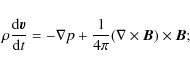
![\begin{displaymath}%
\frac{\partial \vec{B}}{\partial t}=\nabla \times (\vec{v}\...
...\nabla \times \left[ \frac{\vec{j}}{ne}\times \vec{B}\right] ;
\end{displaymath}](/articles/aa/full_html/2010/02/aa12784-09/img24.png)
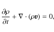
where

The waves in the tube can be excited by the perturbations of the tube end driven by random motions in the photosphere or by magnetic reconnection. Before the waves are excited, the system is assumed to be in quasi-static equilibrium, and the total pressure is set to be constant across the thread. Putting
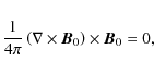
where the subscript 0 refers to the equilibrium state. Equation (5) implies that the equilibrium currents (
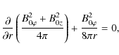
where
We assume that the waves produce small perturbations of the
equilibrium, which allows us to write each physical quantity (except
for the plasma velocity that is set to zero in the equilibrium) as a
sum of a background quantity (denoted with the subscript 0) and a small
perturbation:
| (8) |
To find the governing equation for torsional Alfvén waves, we introduce (7)-(9) into (1)-(3), retaining both background quantities and perturbations. Because the perturbations are small, we apply a standard procedure of linearization, neglecting nonlinear terms (products of perturbations):
![\begin{displaymath}%
\frac{\partial \vec{b}}{\partial t}=\nabla \times \left(\ve...
...}\times \vec{b}+\frac{\vec{j}}{n_{0}e}\times \vec{B}_0\right];
\end{displaymath}](/articles/aa/full_html/2010/02/aa12784-09/img39.png)
where the quantities with subscript 0 are background quantities and the rest are perturbations. Then we linearize the derivative of (4) with respect to time, which gives
Eliminating

As the plasma is homogeneous in the z direction, the perturbations can be Fourier-analysed in z. Since we are interested in the torsional waves with the azimuthal wave number m=0, the wave quantities have the following form:
|
(15) |
where
Before going further, we have to clarify the notions that we use. The
notion of magnetic shear wave defines a wave in which the wave magnetic
fields are normal to the local gradients of the wave profile, such that
there are no compressive magnetic and velocity perturbations but only
shear ones. In ideal MHDs, the torsional Alfvén wave has only
![]() and
and
![]() components.
The torsional wave with m=0 is also a shear wave, because in any point
components.
The torsional wave with m=0 is also a shear wave, because in any point
![]() the wave quantities
the wave quantities
![]() and
and
![]() are perpendicular to the local gradient of the wave profile, which lies in the z-r plane.
are perpendicular to the local gradient of the wave profile, which lies in the z-r plane.
In the Hall MHD, the m=0 torsional Alfvén wave with
short cross-field wavelengths is strictly speaking no longer a
torsional or shear wave, because it also has the radial (vr and br) and the axial (bz and vz) components, coupled to the main shear/torsional
![]() and
and
![]() components. Nevertheless, since the minor
components vr, br, bz, and vz are much smaller than the main ones, we call this mode torsional.
components. Nevertheless, since the minor
components vr, br, bz, and vz are much smaller than the main ones, we call this mode torsional.
Some simplifying assumptions have to be considered to make the problem analytically tractable. The ones we use are to neglect br and vz. Indeed, putting br to zero can be justified by the equation
![]() ,
which can be written as
,
which can be written as
|
(16) |
implying that
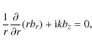
With these approximations, and using (14) to eliminate p, we write the r and ![]() components of Eqs. (10) and (11) as
components of Eqs. (10) and (11) as
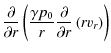
![$\displaystyle +\frac{{\rm i}\omega}{4\pi}\left[\frac{\partial}{\partial r}(B_{0...
...\frac{\partial}{\partial r}\left(r^{2}B_{0\varphi }b_{\varphi}\right)
\right] ;$](/articles/aa/full_html/2010/02/aa12784-09/img59.png)
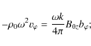
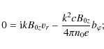
![$\displaystyle +\frac{{\rm i}kc}{4\pi n_{0}e}\left[\frac{\partial}{\partial r}\left(B_{0z}b_{z}\right)+
\frac{2}{r}B_{0\varphi}b_{\varphi}\right] ,$](/articles/aa/full_html/2010/02/aa12784-09/img64.png)
where 0 in subscripts indicates background quantities.
Next, we reduce the set of Eqs. (17)-(20) to one differential equation. We multiply (17) by
![]() and (20) by
and (20) by
![]() ,
and then subtract eliminating bz. The result is
,
and then subtract eliminating bz. The result is
From (18) and (19), we express

Using (22) and (23) in (21), we obtain the following equation for vr:
|
(24) |
Here

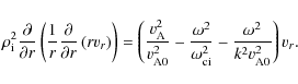
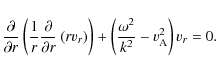
This is the eigenmode equation for torsional Alfvén waves in current threads. It gives the equation for the wave amplitude in r when the Larmor radius
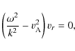
|
(26) |
which is the ideal MHD equation for torsional Alfvén waves in inhomogeneous axially symmetric plasma structures. This equation is singular, giving an infinite number of degenerate solutions and a continuous spectrum.
It is useful to write Eq. (25) in a dimensionless form, where all velocities (including ![]() )
are made dimensionless by the Alfvén velocity
)
are made dimensionless by the Alfvén velocity
![]() ,
distances by the ion gyroradius
,
distances by the ion gyroradius
![]() ,
and magnetic fields by B0z(0) - the value of the background magnetic field at r=0. Thus we write the governing equation in the dimensionless form as
,
and magnetic fields by B0z(0) - the value of the background magnetic field at r=0. Thus we write the governing equation in the dimensionless form as
3 Results
In this section we present the solutions of the (27)
obtained for two particular profiles of the magnetic field. First we
specify the loop parameters, used to calculate the dimensional
quantities, defined at the end of the previous section. The number
density inside and outside the loop is
![]() cm-3, the temperature is
cm-3, the temperature is
![]() K, and the magnetic field at r=0 is
B0z(0)=50 Gauss. Hence,
K, and the magnetic field at r=0 is
B0z(0)=50 Gauss. Hence,
![]() cm/s and
cm/s and
![]() cm.
cm.
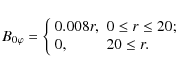
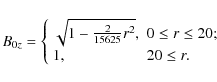
A. The first profile for the magnetic field is

Using this profile for
|
(29) |
Both components of the magnetic field are shown in Fig. 2. It can be seen that, as r increases, B0z decreases to a minimum at r=15 gyroradii, then goes up again until it reaches a constant plateau. For r>20 gyroradii, B0z is constant. At r=0
![\begin{figure}
\par\includegraphics[width=7.5cm,clip]{aa12784-09-fig2.eps}
\end{figure}](/articles/aa/full_html/2010/02/aa12784-09/img92.png)
|
Figure 2:
The plot of B0z (solid line) and
|
| Open with DEXTER | |
For the profile (28), the piecewise solutions to Eq. (27), which are regular at the origin and zero at infinity, are given by the expressions:
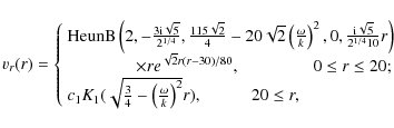
|
(30) |
where HeunB is a bi-confluent Heun function, K1 is the first-order Kummer function. The phase speed
![\begin{figure}
\par\includegraphics[width=7cm,clip]{aa12784-09-fig3.eps}
\end{figure}](/articles/aa/full_html/2010/02/aa12784-09/img98.png)
|
Figure 3:
The dispersion function as a function of the phase velocity,
|
| Open with DEXTER | |
![\begin{figure}
\par\includegraphics[width=7cm,clip]{aa12784-09-fig4.eps}
\end{figure}](/articles/aa/full_html/2010/02/aa12784-09/img99.png)
|
Figure 4:
The amplitude of the radial velocity, vr(r) for case A. Here vr(r) is made dimensionless by the Alfvén velocity,
|
| Open with DEXTER | |
The profile for vr(r), corresponding to the mode with
![]() (which is also the fundamental mode), is plotted in Fig. 4, after c1 was calculated from the boundary conditions. It can be seen from Fig. 4
that the amplitude of the mode reaches a maximum in the interior of the
cylinder. After that, the wave amplitude starts to decrease, going to
zero with growing r.
(which is also the fundamental mode), is plotted in Fig. 4, after c1 was calculated from the boundary conditions. It can be seen from Fig. 4
that the amplitude of the mode reaches a maximum in the interior of the
cylinder. After that, the wave amplitude starts to decrease, going to
zero with growing r.
Next, we define the well-confining condition and calculate the
radius of the cylinder in which the mode is confined well. This is obtained by calculating the safety factor of localization
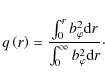
We consider the mode to be localized inside a cylinder with radius
We have to mention that the number of trapped modes depends on the magnitude of the azimuthal field. By increasing
![]() (and hence, the amount of twist), we obtain more modes. We can also
decrease the azimuthal field, such that we do not obtain anymore
trapped modes in the system. For the chosen profile, the modes
disappear if we take 0.023 instead of 0.025 in (28), in front of the
(and hence, the amount of twist), we obtain more modes. We can also
decrease the azimuthal field, such that we do not obtain anymore
trapped modes in the system. For the chosen profile, the modes
disappear if we take 0.023 instead of 0.025 in (28), in front of the
![]() function in the interior on the tube.
function in the interior on the tube.
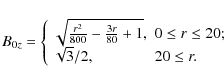
B. The second magnetic field profile we analyse is
|
(32) |
The corresponding B0z, calculated from Eq. (6) is
|
(33) |
This profile is plotted in Fig. 5. It can be seen that
![\begin{figure}
\par\includegraphics[width=7.5cm,clip]{aa12784-09-fig5.eps}
\end{figure}](/articles/aa/full_html/2010/02/aa12784-09/img107.png)
|
Figure 5:
The plot of B0z (full line) and
|
| Open with DEXTER | |
The solutions to Eq. (27) for profile B are
|
(34) |
where M is the Whittaker function, K1 the first-order Kummer function, and c2 the constant to be determined from the matching conditions. The solution satisfies the same boundary conditions: it is regular at the origin and zero at infinity. Applying the same matching conditions at r=20 (the solution is continuous, with continuous derivatives), we find the dispersion equation for
![\begin{figure}
\par\includegraphics[width=7.5cm,clip]{aa12784-09-fig6.eps}
\end{figure}](/articles/aa/full_html/2010/02/aa12784-09/img112.png)
|
Figure 6:
The dispersion function
|
| Open with DEXTER | |
The shape of the eigenmode with the phase speed
![]() is plotted in Fig. 7. It can be seen that it is very similar to the profile of vr obtained in case A: it has a maximum inside the thread, and then goes to zero as r
grows. The difference from case A is that the amplitude now decreases
faster and goes to zero at about 75 gyroradii. This can come from to
the more abrupt magnetic field profile. As in case A, it appears that
the mode is not well confined in the interior of the cylinder. Using
formula 31 we obtain the safety factor q=0.78 for r=20. The radius of the cylinder that confines the mode is
is plotted in Fig. 7. It can be seen that it is very similar to the profile of vr obtained in case A: it has a maximum inside the thread, and then goes to zero as r
grows. The difference from case A is that the amplitude now decreases
faster and goes to zero at about 75 gyroradii. This can come from to
the more abrupt magnetic field profile. As in case A, it appears that
the mode is not well confined in the interior of the cylinder. Using
formula 31 we obtain the safety factor q=0.78 for r=20. The radius of the cylinder that confines the mode is
![]() ,
even closer to the
current thread radius than in case A.
,
even closer to the
current thread radius than in case A.
![\begin{figure}
\par\includegraphics[width=7.5cm,clip]{aa12784-09-fig7.eps}
\end{figure}](/articles/aa/full_html/2010/02/aa12784-09/img115.png)
|
Figure 7:
The amplitude of the radial velocity, vr(r) in r, for case B. Here vr(r) is made dimensionless by
|
| Open with DEXTER | |
In case B, the maximum value of
![]() is 16% of the value of B0z at r=0,
so the field does not need to be as twisted as in the previous example.
However, this profile is not as realistic as the first one. What seems
to be important in obtaining trapped modes is the difference
between the minimum value of B0z inside the tube and the value of B0z outside, which is reflected in the difference in the Alfvén speed. The difference of B0z is about the same in the two cases: 0.9 Gauss for case A and 1.3 Gauss for case B.
is 16% of the value of B0z at r=0,
so the field does not need to be as twisted as in the previous example.
However, this profile is not as realistic as the first one. What seems
to be important in obtaining trapped modes is the difference
between the minimum value of B0z inside the tube and the value of B0z outside, which is reflected in the difference in the Alfvén speed. The difference of B0z is about the same in the two cases: 0.9 Gauss for case A and 1.3 Gauss for case B.
4 Conclusions
In the framework of Hall MHD, we investigated the torsional Alfvén waves in the small-scale current threads in the solar corona. We modelled a thread as a magnetic flux tube with twisted magnetic field lines inside the tube and straight magnetic field lines outside the tube; the density is homogeneous everywhere. The thread's radius is considered to be about 20 gyroradii. We have analysed two particular magnetic field profiles, both localized within r=20 gyroradii.
It was shown that the trapped torsional Alfvén waves can propagate in the current thread with sufficient magnetic twist. The waves propagate along the tube's axis z and have a localized profile across it. The modes are confined in the region of the twisted magnetic field. The wave phase speed is between the minimum value of the Alfvén speed inside the tube and the value of the Alfvén speed outside the tube. Our results show that the number of modes depends on the amount of magnetic twist: the more twisted the tube, the more modes in the system. Also, if the field is not twisted enough the modes can disappear, so there is a threshold twist for their appearance.
The wave profiles we obtained in the present paper are very similar to the wave profiles found in density threads (Copil et al. 2008). In that paper we investigated the trapped torsional Alfvén waves in threads with a homogeneous magnetic field, but inhomogeneous density. The conclusion was that these waves do exist in density threads and are subjected to damping due to viscosity and resistivity. Since the length scales and wave profiles in the current threads are similar to those in the density threads, we suggest that the current thread modes experience a similar damping. It is therefore possible that, as for the density threads, the current threads guiding the torsional Alfvén waves can be places of enhanced coronal heating because of the wave dissipation. However, this has to be analysed quantitatively.
It would also be interesting to study torsional Alfvén waves in threads with both density and magnetic field inhomogeneity to see how these two work together from the point of view of wave trapping and damping.
AcknowledgementsWe thank the referee for constructive criticism that helped us to improve the paper. Y.V. acknowledges partial support by STCE (Solar-Terrestrial Center of Excellence) under the project ``Fundamental science''.
References
- Aschwanden M. J., & Nightingale, R. W. 2005, ApJ, 633, 499 [NASA ADS] [CrossRef] [Google Scholar]
- Aschwanden, M. J., Fletcher, L., Schrijver, C. J., & Alexander, D. 1999, ApJ, 520, 880 [NASA ADS] [CrossRef] [Google Scholar]
- Aschwanden, M. J., Nakariakov, V. M., & Melnikov, V. F. 2004, ApJ, 600, 458 [NASA ADS] [CrossRef] [Google Scholar]
- Banerjee, D., Teriaca, L., Doyle J. G., & Wilhelm, K. 1998, A&A, 339, 208 [NASA ADS] [Google Scholar]
- Copil, P., Voitenko, Y., & Goossens, M. 2008, A&A, 478, 921 [NASA ADS] [CrossRef] [EDP Sciences] [Google Scholar]
- De Moortel, I., Ireland, J., Walsh R. W., & Hood, A. 2002, Sol. Phys., 209, 61 [NASA ADS] [CrossRef] [Google Scholar]
- Dolla, L., & Solomon, J 2008, A&A, 483, 271 [NASA ADS] [CrossRef] [EDP Sciences] [Google Scholar]
- Egan, T. F., & Schneeberger, T. J. 1979, Sol. Phys., 64, 223 [NASA ADS] [CrossRef] [Google Scholar]
- Edwin, P. M., & Roberts, B. 1983, Sol. Phys., 88, 179 [NASA ADS] [CrossRef] [Google Scholar]
- Erdélyi, R., & Carter, B. K. 2006, A&A, 455, 361 [NASA ADS] [CrossRef] [EDP Sciences] [Google Scholar]
- Harrison, R. A., Hood, A. W., & Pike, C. D. 2002, A&A, 392, 319 [NASA ADS] [CrossRef] [EDP Sciences] [Google Scholar]
- Ishii, T. T., Kurokawa, H., & Takeuchi, T. T. 1998, ApJ, 499, 898 [NASA ADS] [CrossRef] [Google Scholar]
- Leka, K. D., Canfield, R. C., McClymont, A. N., & Van Driel-Gesztelyi, L. 1996, 462, 546 [Google Scholar]
- Nakariakov, V. M., Melnikov, V. F., & Reznikova, V. E. 2003, 412, L7 [Google Scholar]
- Nakariakov, V. M., Ofman, L., DeLuca E. E., Roberts, B., & Davila J. M. 1999, Science, 285, 862 [NASA ADS] [CrossRef] [PubMed] [Google Scholar]
- Ofman, L. 2009, ApJ, 694, 502 [NASA ADS] [CrossRef] [Google Scholar]
- Ofman, L., & Wang, T. J. 2008, A&A, 482, L9 [NASA ADS] [CrossRef] [EDP Sciences] [Google Scholar]
- Roberts, B., & Webb, A. R. 1979, Sol. Phys., 64, 77 [NASA ADS] [CrossRef] [Google Scholar]
- Spruit, H. C. 1981, A&A, 102, 129 [NASA ADS] [Google Scholar]
- Spruit, H. C. 1982, Sol. Phys., 75, 3 [NASA ADS] [CrossRef] [Google Scholar]
- Vaiana, G. S., Davis, J. M., Giacconi, R., et al. 1973, ApJ, 185, L47 [NASA ADS] [CrossRef] [Google Scholar]
- Wang, T. J., & Solanki, S. K. 2004, A&A, 421, L33 [NASA ADS] [CrossRef] [EDP Sciences] [Google Scholar]
- Wang, T. J., Solanki, S. K., Innes, D. E., Curdt, W., & Marsch, E. 2003, A&A, 402, L17 [NASA ADS] [CrossRef] [EDP Sciences] [Google Scholar]
- Zaqarashvili, T. V. 2003, A&A, 399, L15 [NASA ADS] [CrossRef] [EDP Sciences] [Google Scholar]
All Figures
|
|
Figure 1:
Model of a current thread. The plasma density is constant everywhere,
but the magnetic field is changing, such that it is straight at r=0, then it twists, and then it is straight again at |
| Open with DEXTER | |
| In the text | |
|
|
Figure 2:
The plot of B0z (solid line) and
|
| Open with DEXTER | |
| In the text | |
|
|
Figure 3:
The dispersion function as a function of the phase velocity,
|
| Open with DEXTER | |
| In the text | |
|
|
Figure 4:
The amplitude of the radial velocity, vr(r) for case A. Here vr(r) is made dimensionless by the Alfvén velocity,
|
| Open with DEXTER | |
| In the text | |
|
|
Figure 5:
The plot of B0z (full line) and
|
| Open with DEXTER | |
| In the text | |
|
|
Figure 6:
The dispersion function
|
| Open with DEXTER | |
| In the text | |
|
|
Figure 7:
The amplitude of the radial velocity, vr(r) in r, for case B. Here vr(r) is made dimensionless by
|
| Open with DEXTER | |
| In the text | |
Copyright ESO 2010
Current usage metrics show cumulative count of Article Views (full-text article views including HTML views, PDF and ePub downloads, according to the available data) and Abstracts Views on Vision4Press platform.
Data correspond to usage on the plateform after 2015. The current usage metrics is available 48-96 hours after online publication and is updated daily on week days.
Initial download of the metrics may take a while.