| Issue |
A&A
Volume 510, February 2010
|
|
|---|---|---|
| Article Number | A3 | |
| Number of page(s) | 25 | |
| Section | Astrophysical processes | |
| DOI | https://doi.org/10.1051/0004-6361/200912473 | |
| Published online | 29 January 2010 | |
Near infrared flares of Sagittarius A*
Importance of near infrared polarimetry
M. Zamaninasab1,2 - A. Eckart1,2 - G. Witzel1 - M. Dovciak3 - V. Karas3 - R. Schödel4 - R. Gießübel1,2 - M. Bremer1 - M. García-Marín1 - D. Kunneriath1,2 - K. Muzic1 - S. Nishiyama5 - N. Sabha1 - C. Straubmeier1 - A. Zensus2,1
1 - I.Physikalisches Institut, Universität zu Köln,
Zülpicher Str.77, 50937 Köln, Germany
2 -
Max-Planck-Institut für Radioastronomie,
Auf dem Hügel 69, 53121 Bonn, Germany
3 -
Astronomical Institute, Academy of Sciences,
Bocní II, 14131 Prague, Czech Republic
4 -
Instituto de Astrofísica de Andalucía -CSIC, Glorieta de la Astronomía S/N, 18008 Granada, Spain
5 -
Department of Astronomy, Kyoto University, Kyoto 606-8502, Japan
Received 12 May 2009 / Accepted 8 November 2009
Abstract
Context. We report on the results of new simulations of
near-infrared (NIR) observations of the Sagittarius A*
(Sgr A*) counterpart associated with the super-massive black hole
at the Galactic Center.
Aims. Our goal is to investigate and understand the physical
processes behind the variability associated with the NIR flaring
emission from Sgr A*.
Methods. The observations have been carried out using the NACO
adaptive optics (AO) instrument at the European Southern Observatory's
Very Large Telescope and CIAO NIR camera on the Subaru telescope (13
june 2004; 30 july 2005; 1 june 2006; 15 may 2007; 17 may 2007 and 28
may 2008). We used a model of synchrotron emission from relativistic
electrons in the inner parts of an accretion disk. The relativistic
simulations have been carried out using the Karas-Yaqoob (KY)
ray-tracing code.
Results. We probe the existence of a correlation between the
modulations of the observed flux density light curves and changes in
polarimetric data. Furthermore, we confirm that the same correlation is
also predicted by the hot spot model. Correlations between intensity
and polarimetric parameters of the observed light curves as well as a
comparison of predicted and observed light curve features through a
pattern recognition algorithm result in the detection of a signature of
orbiting matter under the influence of strong gravity. This pattern is
detected statistically significant against randomly polarized red
noise. Expected results from future observations of VLT interferometry
like GRAVITY experiment are also discussed.
Conclusions. The observed correlations between flux modulations
and changes in linear polarization degree and angle can be a sign that
the NIR flares have properties that are not expected from purely random
red-noise. We find that the geometric shape of the emission region
plays a major role in the predictions of the model. From fully
relativistic simulations of a spiral shape emitting region, we conclude
that the observed swings of the polarization angle during NIR flares
support the idea of compact orbiting spots instead of extended
patterns. The effects of gravitational shearing, fast synchrotron
cooling of the components and confusion from a variable accretion disk
have been taken into account. Simulated centroids of NIR images lead us
to the conclusion that a clear observation of the position wander of
the center of NIR images with future infrared interferometers will
prove the existence of orbiting hot spots in the vicinity of our
Galactic super-massive black hole.
Key words: black hole physics - infrared: general - accretion, accretion disks - Galaxy: center - Galaxy: nucleus
1 Introduction
![\begin{figure}
{\includegraphics[width=18cm,clip]{12473f1.eps} }\end{figure}](/articles/aa/full_html/2010/02/aa12473-09/img66.png)
|
Figure 1:
Sgr A* as it was observed in NIR L'-band
(3.8 |
| Open with DEXTER | |
The nearest super-massive black hole candidate (
![]() )
lies at the center of our galaxy, as inferred from motions
of stars near the Galactic Center (Eckart & Genzel 1996, 1997;
Eckart et al. 2002; Schödel et al. 2002; Eisenhauer et al. 2003;
Ghez et al. 2000, 2005, 2008; Gillessen et al. 2009). With a
luminosity of
)
lies at the center of our galaxy, as inferred from motions
of stars near the Galactic Center (Eckart & Genzel 1996, 1997;
Eckart et al. 2002; Schödel et al. 2002; Eisenhauer et al. 2003;
Ghez et al. 2000, 2005, 2008; Gillessen et al. 2009). With a
luminosity of
![]() ,
where
,
where
![]() is its
limiting Eddington luminosity, Sagittarius A*, the radio source
associated with this SMBH, is one of the most extreme sub-Eddington
sources accessible to observations. However, X-ray and near-infrared
(NIR) flares are routinely detected with high spatial and spectral
resolution observations (Baganoff et al. 2001; Porquet et al. 2003,
2008; Genzel et al. 2003; Eckart et al. 2004, 2006a-c, 2008a-c;
Meyer et al. 2006a,b, 2007; Yusef-Zadeh et al. 2006a,b, 2007, 2008).
These short bursts of increased radiation last normally for about
100 min and occur four to five times a day (see Fig. 1 for a typical
behavior of Sgr A* during a flaring phase in NIR bandwidth).
is its
limiting Eddington luminosity, Sagittarius A*, the radio source
associated with this SMBH, is one of the most extreme sub-Eddington
sources accessible to observations. However, X-ray and near-infrared
(NIR) flares are routinely detected with high spatial and spectral
resolution observations (Baganoff et al. 2001; Porquet et al. 2003,
2008; Genzel et al. 2003; Eckart et al. 2004, 2006a-c, 2008a-c;
Meyer et al. 2006a,b, 2007; Yusef-Zadeh et al. 2006a,b, 2007, 2008).
These short bursts of increased radiation last normally for about
100 min and occur four to five times a day (see Fig. 1 for a typical
behavior of Sgr A* during a flaring phase in NIR bandwidth).
Recent NIR and X-ray observations have revealed the non-thermal
nature of high frequency radiation from Sgr A* (Eckart et al. 2006a-c, 2008a-c; Gillessen et al. 2006; Hornstein et al. 2007).
Sgr A* is probably visible in the NIR regime only during its flaring
state. The short time scale variabilities seen during several
observed NIR and X-ray flares argue for an emitting region not
bigger than about ten Schwarzschild radii
(
![]() cm) of the associated super-massive black hole
(Baganoff et al. 2001; Genzel et al. 2003). We have scaled the
relevant physical distances according to the gravitational radius
(
cm) of the associated super-massive black hole
(Baganoff et al. 2001; Genzel et al. 2003). We have scaled the
relevant physical distances according to the gravitational radius
(![]() )
throughout this paper. The NIR flares are highly polarized
and normally have X-ray counterparts, which strongly suggests a
synchrotron-self-Compton (SSC) or inverse Compton emission as the
responsible radiation mechanism (Eckart et al. 2004, 2006a,b; Yuan et al. 2004; Liu et al. 2006). Several observations have already
confirmed the existence of a time lag between the simultaneous
NIR/X-ray flares and the flares in the lower frequencies. This is
interpreted as a sign for cooling down via adiabatic expansion
(Eckart et al. 2006a, 2008b,c; Yusef-Zadeh et al. 2006a,b, 2007,
2008; Marrone et al. 2008, Zamaninasab et al. 2008a).
)
throughout this paper. The NIR flares are highly polarized
and normally have X-ray counterparts, which strongly suggests a
synchrotron-self-Compton (SSC) or inverse Compton emission as the
responsible radiation mechanism (Eckart et al. 2004, 2006a,b; Yuan et al. 2004; Liu et al. 2006). Several observations have already
confirmed the existence of a time lag between the simultaneous
NIR/X-ray flares and the flares in the lower frequencies. This is
interpreted as a sign for cooling down via adiabatic expansion
(Eckart et al. 2006a, 2008b,c; Yusef-Zadeh et al. 2006a,b, 2007,
2008; Marrone et al. 2008, Zamaninasab et al. 2008a).
The other feature related to these NIR/X-ray flares are the
claimed quasi-periodic oscillations (QPOs) with a period of ![]() min, which have been reported in several of these events
(Genzel et al. 2003; Belanger et al. 2006; Eckart et al. 2006b,c;
2008a; Meyer et al. 2006a,b, Hamaus et al. (2009)).
Short periods of
increased radiation (the so called ``NIR flares'', normally around
100 min) seem to be accompanied by QPOs. All the studies mentioned
above probed this
min, which have been reported in several of these events
(Genzel et al. 2003; Belanger et al. 2006; Eckart et al. 2006b,c;
2008a; Meyer et al. 2006a,b, Hamaus et al. (2009)).
Short periods of
increased radiation (the so called ``NIR flares'', normally around
100 min) seem to be accompanied by QPOs. All the studies mentioned
above probed this ![]() min quasi-periodicity, by performing a sliding window analysis with
window lengths of the order of the flaring time. Recently, Do et al. (2009) argued that they did not find any significant periodicity at
any time scale while probing their sample of observations for a
periodic signal. Their method is based on the Lomb-Scargle
periodogram analysis of a sample of six light curves and comparing
them with several thousands of artificial light curves with the same
underlying red-noise. One must note that the suggested
QPOs are transient phenomena, lasting for only very few cycles
(50-100 min). This kind of behavior, along with the inevitable
uncertainty in the red noise power law index determination, makes a
clear and unambiguous detection (
min quasi-periodicity, by performing a sliding window analysis with
window lengths of the order of the flaring time. Recently, Do et al. (2009) argued that they did not find any significant periodicity at
any time scale while probing their sample of observations for a
periodic signal. Their method is based on the Lomb-Scargle
periodogram analysis of a sample of six light curves and comparing
them with several thousands of artificial light curves with the same
underlying red-noise. One must note that the suggested
QPOs are transient phenomena, lasting for only very few cycles
(50-100 min). This kind of behavior, along with the inevitable
uncertainty in the red noise power law index determination, makes a
clear and unambiguous detection (
![]() )
of a periodic signal very
difficult. Whenever a flare of Sgr A* was observed with polarimetry,
it was found that it is accompanied by significant polarization which
varies on similarly short timescales as the light curve itself. By carrying
out an analysis only on the total flux, some pieces of
the observed information are ignored. It is already known that
polarimetric data have been shown to be able to reveal substructure
in flares, even when the light curve appears largely featureless
(e.g. see Fig. 4 in Eckart et al. 2006b). The other main advantage
of polarimetric observations is that, in addition to the flux
density light curve, one can analyze the changes in the observed
degree of polarization and the changes in polarization angle
during flaring time as well.
)
of a periodic signal very
difficult. Whenever a flare of Sgr A* was observed with polarimetry,
it was found that it is accompanied by significant polarization which
varies on similarly short timescales as the light curve itself. By carrying
out an analysis only on the total flux, some pieces of
the observed information are ignored. It is already known that
polarimetric data have been shown to be able to reveal substructure
in flares, even when the light curve appears largely featureless
(e.g. see Fig. 4 in Eckart et al. 2006b). The other main advantage
of polarimetric observations is that, in addition to the flux
density light curve, one can analyze the changes in the observed
degree of polarization and the changes in polarization angle
during flaring time as well.
The claimed quasi-periodicity has been interpreted as being related to the orbital time scale of the matter in the inner parts of the accretion disk. According to well-known observed high frequency quasi-periodic oscillations (HFQPOs) in X-ray light curves of stellar mass black holes and binaries (Nowak & Lehr 1998), this interpretation is of special interest since it shows a way to better understand the behavior of accretion disks for a wide range of black hole masses. The recent unambiguous discovery of a one hour (quasi-)periodicity in the X-ray emission light curve of the active galaxy RE J1034+396 provides further support to this idea and extends the similarity between stellar-mass and super-massive black holes to a new territory (Gierlinski et al. 2008).
Although the origin of the observed QPOs in the sources associated
with black holes is still a matter of debate, several
magnetohydrodynamic (MHD) simulations confirmed that it could be
related to instabilities in the inner parts of the accretion disks,
very close to the marginally stable orbit of the black hole
(
![]() ), and also possibly connected with the so-called ``stress
edge'' (Hawley 1991; Chan et al. 2009b). If the flux modulations are
related to a single azimuthal compact over-dense region (hereafter:
``hot spot''), orbiting with the same speed as the underlying
accretion disk, one can constrain the spin of the black hole by
connecting the observed time scales of QPOs to the orbital time
scale of matter around the black hole:
), and also possibly connected with the so-called ``stress
edge'' (Hawley 1991; Chan et al. 2009b). If the flux modulations are
related to a single azimuthal compact over-dense region (hereafter:
``hot spot''), orbiting with the same speed as the underlying
accretion disk, one can constrain the spin of the black hole by
connecting the observed time scales of QPOs to the orbital time
scale of matter around the black hole:
![]() min (Bardeen et al. 1972, where
min (Bardeen et al. 1972, where
![]() is the black hole dimensionless
spin parameter and r is the distance of the spot from the black
hole). The characteristic behavior of general relativistic flux
modulations produced via the orbiting hot spots have been discussed
in several papers (see e.g. Cunningham & Bardeen 1973; Abramowicz
et al. 1991; Karas & Bao 1992; Hollywood et al. 1995; Dovciak
2004, 2007). In this paper, we have used a spotted accretion disk
scenario to model the observed patterns of our sample of NIR
light curves.
is the black hole dimensionless
spin parameter and r is the distance of the spot from the black
hole). The characteristic behavior of general relativistic flux
modulations produced via the orbiting hot spots have been discussed
in several papers (see e.g. Cunningham & Bardeen 1973; Abramowicz
et al. 1991; Karas & Bao 1992; Hollywood et al. 1995; Dovciak
2004, 2007). In this paper, we have used a spotted accretion disk
scenario to model the observed patterns of our sample of NIR
light curves.
Table 1: Observations log.
Several authors have proposed different models in order to explain the flaring activity of Sgr A*. These models cover a wide range of hypotheses like disk-star interactions (Nayakshin et al. 2004), stochastic acceleration of electrons in the inner region of the disk (Liu et al. 2006), sudden changes in the accretion rate of the black hole (Liu et al. 2002), heating of electrons close to the core of a jet (Markoff et al. 2001; Yuan et al. 2002), trapped oscillatory modes in the inner regions of the accretion disk in the form of spiral patterns or Rossby waves (Tagger & Melia 2006; Falanga et al. 2007; Karas et al. 2008), non-axisymmetric density perturbations which emerge as the disk evolves in time (Chan et al. 2009b), non-Keplerian orbiting spots falling inward inside the plunging region created via magnetic reconnections (Falanga et al. 2008), and also comet like objects trapped and tidally disrupted by the black hole (Cadez et al. 2006; Kostic et al. 2009).
Observational data render some of these models unlikely. The star-disk interaction model is unable to produce the repeated flux modulations and also the high degree of polarization since it mainly deals with thermal emission. Tidal disruption of comet-like objects are also unable to reproduce the observed rate of flares per day, since the estimated capture rate of such objects for the Sgr A* environment is at least one order of magnitude lower (Cadez et al. 2006; this is a very rough estimate. The actual capture rate of such objects can not be well determined (A. Cadez, private communication)). Nevertheless, several viable models exist and make different predictions that can be distinguished observationally. For example, one important characteristic prediction of hot spot models is about the wobbling of the center of the images (Broderick & Loeb 2006a,b; Paumard et al. 2006; Zamaninasab et al. 2008b; Hamaus et al. 2009). Significant effort has been already devoted to measure this possible position wander of Sgr A* in the mm, sub-mm and NIR regimes (Eisenhauer 2005b, 2008; Gillessen 2006; Reid et al. 2008; Doelleman et al. 2008). In this paper we discuss how NIR polarimetry and the next generations of VLT interferometry (VLTI) and Very Long Baseline Interferometry (VLBI) experiments can provide data to support or reject certain models for the accretion flow/outflow related to Sgr A*. Obtaining accurate data on the accretion flow of Sgr A* can lead us to a better understanding of the physics of strong gravitational regimes, formation of black holes and their possible relation to the galaxy formation process in a cosmological context.
In Sect. 2 we present a complete sample of NIR light curves observed in the polarimetry mode. A brief description about the details of the observation and data reduction methods is provided. We discuss the quasi-periodicity detection methods and present the results of a correlation analysis between the flux and polarimetric parameters. A general description of our model setup and results of simulations are discussed in Sect. 3. We show how NIR polarimetry can be used as a way to constrain physical parameters of the emitting region (like its geometrical shape) in Sect. 4 and Sect. 5. In Sect. 6 we mainly discuss the predictions that the future NIR interferometer (GRAVITY) is expected to reveal and how different assumptions in the model parameters can modify the results. In Sect. 7 we summarize the main results of the paper and draw our conclusions.
2 NIR polarimetry
2.1 Observations and data reduction
All observations we refer to in this paper have been carried
out in the NIR Ks band with the NIR camera CONICA and the
adaptive optics (AO) module NAOS (NACO) at the ESO VLT unit
telescope 4 (YEPUN) on Paranal, Chile![]() and CIAO NIR camera on the Subaru telescope
and CIAO NIR camera on the Subaru telescope![]() . These
facilities are suited for both time resolved observations of total
intensity and polarimetric degree and angle with a sampling
of about two to three minutes. The NAOS/CONICA NIR camera installed on
UT4, VLT allows for a simultaneous measurement of two orthogonal
directions of electric field vector via a Wollaston prism. The
combination with a rotary half-wave plate allows the rapid alternation
between measurements of different angles of the electric
vector. This is crucial for determining the linear polarization
characteristics of a time-varying source. The CIAO camera uses a
rotating half-wave plane combined with a fixed wire grid polarizer
for measuring the linear polarization.
. These
facilities are suited for both time resolved observations of total
intensity and polarimetric degree and angle with a sampling
of about two to three minutes. The NAOS/CONICA NIR camera installed on
UT4, VLT allows for a simultaneous measurement of two orthogonal
directions of electric field vector via a Wollaston prism. The
combination with a rotary half-wave plate allows the rapid alternation
between measurements of different angles of the electric
vector. This is crucial for determining the linear polarization
characteristics of a time-varying source. The CIAO camera uses a
rotating half-wave plane combined with a fixed wire grid polarizer
for measuring the linear polarization.
Since the
first NIR polarimetric observation of Sgr A* in 2004 (Eckart et al.
2006a), several polarized flares have been observed (Meyer et al.
2006a,b, 2007; Eckart et al. 2008a). In the VLT observations, the
infrared wavefront sensor of NAOS was used to lock the AO loop on
the NIR bright (K-band magnitude ![]() )
supergiant IRS 7,
located about 5.6'' north of Sgr A*. Atmospheric conditions (and
consequently the AO correction) were stable enough during the
observations for doing high angular resolution photometry and
polarimetry (with a typical coherence time of 2 milliseconds and larger).
The exposures have been dithered. The reductions of the 1 june 2006
and 15 may 2007 data presented here have been repeated for this
publication to confirm the significance of the discussed features
(see also Eckart et al. 2008a). The 17 may
2007 data have not been published before. All exposures were sky
subtracted, flat-fielded, and corrected for dead or bad pixels. As
the most important improvement of the new reduction the dithered
exposures have been aligned with sub-pixel accuracy by a
cross-correlation method (Devillard 1999). PSFs were extracted from
these images with StarFinder (Diolaiti et al. 2000). The images were
deconvolved with the Lucy-Richardson (LR) algorithm. Beam
restoration was carried out with a Gaussian beam of FWHM
corresponding to the respective wavelength. The final resolution at
)
supergiant IRS 7,
located about 5.6'' north of Sgr A*. Atmospheric conditions (and
consequently the AO correction) were stable enough during the
observations for doing high angular resolution photometry and
polarimetry (with a typical coherence time of 2 milliseconds and larger).
The exposures have been dithered. The reductions of the 1 june 2006
and 15 may 2007 data presented here have been repeated for this
publication to confirm the significance of the discussed features
(see also Eckart et al. 2008a). The 17 may
2007 data have not been published before. All exposures were sky
subtracted, flat-fielded, and corrected for dead or bad pixels. As
the most important improvement of the new reduction the dithered
exposures have been aligned with sub-pixel accuracy by a
cross-correlation method (Devillard 1999). PSFs were extracted from
these images with StarFinder (Diolaiti et al. 2000). The images were
deconvolved with the Lucy-Richardson (LR) algorithm. Beam
restoration was carried out with a Gaussian beam of FWHM
corresponding to the respective wavelength. The final resolution at
![]() m is about 60 milli-arcseconds (mas). Flux densities of the
sources were measured by aperture photometry. Because of the high
accuracy of the image alignment it was possible to separate Sgr A*
from the nearby stars S17 and S13 by choosing a circular aperture of
about 52 mas radius (see Fig. 15 of Eckart et al. 2006a, and
discussion therein), resulting in a better correction for the flux
contribution of these stars. The data was corrected for extinction
using AK = 2.8 (Eisenhauer et al. 2005a; Schödel et al.
2007). The relative flux density calibration was carried out using
known K-band flux densities and positions of 14 sources in the IRS16
cluster by
R. Schödel (private communications). This results in a K-band flux of
the high velocity star S2 of
m is about 60 milli-arcseconds (mas). Flux densities of the
sources were measured by aperture photometry. Because of the high
accuracy of the image alignment it was possible to separate Sgr A*
from the nearby stars S17 and S13 by choosing a circular aperture of
about 52 mas radius (see Fig. 15 of Eckart et al. 2006a, and
discussion therein), resulting in a better correction for the flux
contribution of these stars. The data was corrected for extinction
using AK = 2.8 (Eisenhauer et al. 2005a; Schödel et al.
2007). The relative flux density calibration was carried out using
known K-band flux densities and positions of 14 sources in the IRS16
cluster by
R. Schödel (private communications). This results in a K-band flux of
the high velocity star S2 of ![]() mJy, which compares well with
the magnitudes and fluxes for S2 quoted by Ghez et al. (2005b) and
Genzel et al. (2003). The measurement uncertainties for Sgr A* were
obtained from the reference star S2. For more details about CIAO
observations see Nishiyama et al. (2009).
mJy, which compares well with
the magnitudes and fluxes for S2 quoted by Ghez et al. (2005b) and
Genzel et al. (2003). The measurement uncertainties for Sgr A* were
obtained from the reference star S2. For more details about CIAO
observations see Nishiyama et al. (2009).
2.2 Data analysis
2.2.1 Periodicity
Figure 2 shows flare events observed in the NIR K-band
(2.2 ![]() m) on 13 june 2004; 30 july 2005; 1 june 2006; 15 may 2007;
17 may 2007 and 28 may 2008. This sample includes all flare events
observed in NIR polarimetry during recent years according to the
knowledge of the authors. The flux densities rise and come back to their
quiescent level in time intervals of roughly 100 min. The
measured values of total flux, degree of polarization, and angle of
polarization vary significantly on time scales of
m) on 13 june 2004; 30 july 2005; 1 june 2006; 15 may 2007;
17 may 2007 and 28 may 2008. This sample includes all flare events
observed in NIR polarimetry during recent years according to the
knowledge of the authors. The flux densities rise and come back to their
quiescent level in time intervals of roughly 100 min. The
measured values of total flux, degree of polarization, and angle of
polarization vary significantly on time scales of ![]() 10 min.
These abrupt changes can be more clearly detected when the events
are in their brightest state. Even if the flares are different in
some aspects (e.g. the ratio of the changes of the flux, the maximum
brightness achieved, or the degree of linear polarization), there
could exist some features that are repeated
in our sample. Here we perform a quantitative analysis in
order to probe such features. We focus first on detecting periodic
signatures in flux densities and then a possible correlation between
changes in flux and polarimetric light curves.
10 min.
These abrupt changes can be more clearly detected when the events
are in their brightest state. Even if the flares are different in
some aspects (e.g. the ratio of the changes of the flux, the maximum
brightness achieved, or the degree of linear polarization), there
could exist some features that are repeated
in our sample. Here we perform a quantitative analysis in
order to probe such features. We focus first on detecting periodic
signatures in flux densities and then a possible correlation between
changes in flux and polarimetric light curves.
The autocorrelation function and Lomb-Scargle periodograms can be used to detect signatures of time periodic structures. For the autocorrelation analysis we used the z-transformed discrete correlation function (ZDCF) algorithm (Alexander 1997), which is particularly useful for analyzing sparse, unevenly sampled light curves. For Lomb-Scargle periodograms we followed Press & Rybicki (1989).
![\begin{figure}
{\includegraphics[width=18cm,clip]{12473f2.eps} }\end{figure}](/articles/aa/full_html/2010/02/aa12473-09/img79.png)
|
Figure 2:
Our sample of light curves of Sgr A* flares
observed in NIR Ks band (2.2 |
| Open with DEXTER | |
![\begin{figure}
{\includegraphics[width=18cm,clip]{12473f3.eps} }\end{figure}](/articles/aa/full_html/2010/02/aa12473-09/img80.png)
|
Figure 3:
ZDCF of the flux light curves of 13 june 2004 a);
30 july 2005 b); 1 june 2006 c); 15 may 2007 d); 17 may 2007 e)
and 28 may 2008 f). The vertical colored boxes indicate the
position of the closest peaks to the zero time lags. Dotted lines
show the median (red), |
| Open with DEXTER | |
Figure 3 shows the cross-correlation of the flux
density light curves of our sample with themselves by using ZDCF
method. The ZDCF of the 30 july 2005; 1 june 2006; 15 and 17 may 2007
flares show peaks around ![]() min time-lag, and specially for 15
and 17 may 2007 the peaks look significant. These peaks can be signs
of a possible periodicity.
min time-lag, and specially for 15
and 17 may 2007 the peaks look significant. These peaks can be signs
of a possible periodicity.
As one can see, only 17 may 2007's ZDCF shows a peak above
the ![]() significance threshold. The false alarm values have
been derived by repeating the same ZDCF analysis on the 104random red-noise light curves. The criteria for this comparison and
the way the light curves are produced are described below. Here we
must note that since the ZDCF values are normalized and distributed
in a [-1:1] interval, the distribution of the values for each time lag
(
significance threshold. The false alarm values have
been derived by repeating the same ZDCF analysis on the 104random red-noise light curves. The criteria for this comparison and
the way the light curves are produced are described below. Here we
must note that since the ZDCF values are normalized and distributed
in a [-1:1] interval, the distribution of the values for each time lag
(![]() )
is not Gaussian (see Fig. 4). As a result we
have used the median and percentile nomenculture instead of the
normal standard deviation formalism for deriving the false alarm
levels.
)
is not Gaussian (see Fig. 4). As a result we
have used the median and percentile nomenculture instead of the
normal standard deviation formalism for deriving the false alarm
levels.
We have highlighted the time windows in which ZDCFs show a peak
around ![]() min, coinciding with the claimed quasi-periodicity.
Even though the 1 june 2006 and 15 may 2007's ZDCFs do not show peaks
above
min, coinciding with the claimed quasi-periodicity.
Even though the 1 june 2006 and 15 may 2007's ZDCFs do not show peaks
above ![]() significance, they however still reach
significance, they however still reach ![]() and
and
![]() levels, respectively. Also, by a rough estimate, the
significance of the ZDCF peaks are correlated to the brightness of
the flares, and for the faint events, as is observed for example in
2004, there is no detectable peak.
levels, respectively. Also, by a rough estimate, the
significance of the ZDCF peaks are correlated to the brightness of
the flares, and for the faint events, as is observed for example in
2004, there is no detectable peak.
Figure 5 shows the Lomb-Scargle periodogram for each
flux light curve. The usual factor of four times over-sampling was
applied in order to increase the sensitivity. All periodograms show the
power law behavior,
![]() ,
showing
greater power at lower frequencies. Here
,
showing
greater power at lower frequencies. Here
![]() is power, fis frequency and
is power, fis frequency and ![]() is power law index. All light curves
follow a red noise under-lying power spectral density (PSD) with
is power law index. All light curves
follow a red noise under-lying power spectral density (PSD) with
![]() .
To test the significance of the peaks in
the periodogram we have repeated the Lomb-Scargle analysis for
104 simulated red noise light curves. For simulating the red
noise we have followed the algorithm by Trimmer and König (1995)
(see Figs. 9-11 for
examples). The red noise light curves were produced for each event
separately following the procedure below: (1) Determining the slope
of the observed PSD for each event using a linear fit to the
periodogram in log-log space and also by fitting a first-order
autoregressive function to the PSD (Schulz & Mudelsee 2002) and
averaging the results of both methods (the resulted
.
To test the significance of the peaks in
the periodogram we have repeated the Lomb-Scargle analysis for
104 simulated red noise light curves. For simulating the red
noise we have followed the algorithm by Trimmer and König (1995)
(see Figs. 9-11 for
examples). The red noise light curves were produced for each event
separately following the procedure below: (1) Determining the slope
of the observed PSD for each event using a linear fit to the
periodogram in log-log space and also by fitting a first-order
autoregressive function to the PSD (Schulz & Mudelsee 2002) and
averaging the results of both methods (the resulted ![]() is
presented in the lower right corner of each plot in Fig. 5).
(2) 104 red noise light curves produced with the related
is
presented in the lower right corner of each plot in Fig. 5).
(2) 104 red noise light curves produced with the related ![]() following the method of Timmer & König (1995). The light
curves have been produced by selecting a middle part of a light
curve with a length at least ten times longer than the observed light
curve following the argument by Uttley et al. (2002). The selected
segment of the light curve is sampled to the same time bin of the
corresponding observation. This will correct for any artificial
effects caused by time lags which exist on our light curves and also
the uneven sampling of our observations. (3) The value of the flux
has multiplied by one factor as the mean of the simulated flux has the
same value as the observational one for each night.
following the method of Timmer & König (1995). The light
curves have been produced by selecting a middle part of a light
curve with a length at least ten times longer than the observed light
curve following the argument by Uttley et al. (2002). The selected
segment of the light curve is sampled to the same time bin of the
corresponding observation. This will correct for any artificial
effects caused by time lags which exist on our light curves and also
the uneven sampling of our observations. (3) The value of the flux
has multiplied by one factor as the mean of the simulated flux has the
same value as the observational one for each night.
None of the periodograms of Fig. 5 show a peak that
exceeds the ![]() threshold except the ones correlated to the
lengths of the flare events (
threshold except the ones correlated to the
lengths of the flare events (![]() 100 min). We specially
highlighted the windows in which corresponding ZDCFs peak. In order
to see if there exists a persistent frequency peak in the PSDs, we
averaged all observed periodograms (Fig. 6b). The average periodogram doesn't show a significant peak in
comparison with the false alarm level even if we exclude the 13
june 2004 light curve (Fig. 6c). As we mentioned
before the short time scale of the flares and limited number of
cycles make a significant detection of any periodicity very
difficult. In addition, the possible quasi-periodic structure can vary
during the time of the flare if it is connected to the falling
clumps of matter into the black hole (Falanga et al. 2008). In this
case the Lomb-Scargle algorithm finds different frequencies and
allocates them separate values of power. This effect can result in a
periodogram in which the values of power are higher in a band of
frequencies instead of a specific value. As one can see in
Fig. 5, 1 june 2006 and 15 may 2007 can be the candidates for
such an effect since the value of the PSD function remains high in the
highlighted window. To test for such an effect we averaged the
periodograms with a new bin size and repeated the same procedure for
the random red noise PSDs (Fig. 7). The resulting
averaged periodogram does not show any significant peak again (Fig. 7b), even if we exclude the 13 june 2004 event
(Fig. 7c). Since this procedure is very sensitive
to the size of the chosen window (which can vary from event to
event), a more detailed analysis is needed to study the possible
evolution of any periodic signal.
100 min). We specially
highlighted the windows in which corresponding ZDCFs peak. In order
to see if there exists a persistent frequency peak in the PSDs, we
averaged all observed periodograms (Fig. 6b). The average periodogram doesn't show a significant peak in
comparison with the false alarm level even if we exclude the 13
june 2004 light curve (Fig. 6c). As we mentioned
before the short time scale of the flares and limited number of
cycles make a significant detection of any periodicity very
difficult. In addition, the possible quasi-periodic structure can vary
during the time of the flare if it is connected to the falling
clumps of matter into the black hole (Falanga et al. 2008). In this
case the Lomb-Scargle algorithm finds different frequencies and
allocates them separate values of power. This effect can result in a
periodogram in which the values of power are higher in a band of
frequencies instead of a specific value. As one can see in
Fig. 5, 1 june 2006 and 15 may 2007 can be the candidates for
such an effect since the value of the PSD function remains high in the
highlighted window. To test for such an effect we averaged the
periodograms with a new bin size and repeated the same procedure for
the random red noise PSDs (Fig. 7). The resulting
averaged periodogram does not show any significant peak again (Fig. 7b), even if we exclude the 13 june 2004 event
(Fig. 7c). Since this procedure is very sensitive
to the size of the chosen window (which can vary from event to
event), a more detailed analysis is needed to study the possible
evolution of any periodic signal.
![\begin{figure}
{\includegraphics[width=8cm,clip]{12473f4n.eps} }\end{figure}](/articles/aa/full_html/2010/02/aa12473-09/img87.png)
|
Figure 4:
ZDCF of 104 simulated red noise light curves
overplotted in one image a). The resulted average and standard
deviation as well as the median and percentile values are presented.
The distribution of the ZDCF values for different time lags ( |
| Open with DEXTER | |
2.2.2 Importance of polarimetry
We have also performed cross correlation analysis between
variations of flux and degree (angle) of polarization. A search for
any short time-lag correlation has been carried out by scanning the
light curves using a sliding window method (see Fig. 12a). The size of the scanning window
(![]() )
is fixed on 40 min since we are interested in
magnifying any short lag correlation related to the possible
)
is fixed on 40 min since we are interested in
magnifying any short lag correlation related to the possible
![]() min quasi-periodicity. Figure 8 shows the
cross-correlations of the two sets of mentioned light curves for all
events in our sample. The time steps of the scans were fixed to be five
minutes. The presented results are the average of all scans weighted
by the flare signal to noise ratio (i.e. each part of the flare that
is brighter, has more weight). Since the ZDCF algorithm needs at
least 11 points per bin for reliable results (specially for the
error estimation; see Alexander 1997) a linear interpolation of the
polarimetric data points has been performed. We must mention that
due to the confusion from nearby stars and the diffuse background
emission the accuracy of measuring polarimetric parameters is
related to the brightness of Sgr A*. This means that the most
reliable polarimetric data are measured when strong flares happen,
specially when the source is in its brightest state.
min quasi-periodicity. Figure 8 shows the
cross-correlations of the two sets of mentioned light curves for all
events in our sample. The time steps of the scans were fixed to be five
minutes. The presented results are the average of all scans weighted
by the flare signal to noise ratio (i.e. each part of the flare that
is brighter, has more weight). Since the ZDCF algorithm needs at
least 11 points per bin for reliable results (specially for the
error estimation; see Alexander 1997) a linear interpolation of the
polarimetric data points has been performed. We must mention that
due to the confusion from nearby stars and the diffuse background
emission the accuracy of measuring polarimetric parameters is
related to the brightness of Sgr A*. This means that the most
reliable polarimetric data are measured when strong flares happen,
specially when the source is in its brightest state.
![\begin{figure}
{\includegraphics[width=18cm,clip]{12473f5.eps} }
\end{figure}](/articles/aa/full_html/2010/02/aa12473-09/img88.png)
|
Figure 5:
Lomb-Scargle periodograms of the flux light curves
for 13 june 2004 a); 30 july 2005 b); 1 june 2006 c); 15 may 2007
d); 17 may 2007 e) and 28 may 2008 f). The dashed lines show the
median (red) and , |
| Open with DEXTER | |
In order to test whether a random red noise model can
produce the same correlation patterns we need to simulate red noise
light curves including polarimetric data. For this purpose, we have
simulated random E vectors for four perpendicular directions:
| (1) |
where
| F | = | F0+F90 | (2) |
| Q | = | F0-F90 | (3) |
| U | = | F45-F135 | (4) |
| = | (5) | ||
| = | 
|
(6) |
(where F is the total flux, Q and U are the Stokes parameters,
![\begin{figure}
{\includegraphics[width=8.5cm,clip]{12473f6.eps} }\end{figure}](/articles/aa/full_html/2010/02/aa12473-09/img101.png)
|
Figure 6:
Lomb-Scargle periodograms of the flux light curves
of our sample overplotted in the same plot a). Averaged result of
all periodograms b) and excluding the 13 june 2004 flare
c). Highlighted box shows the expected |
| Open with DEXTER | |
![\begin{figure}
{\includegraphics[width=8.5cm,clip]{12473f7.eps} }\end{figure}](/articles/aa/full_html/2010/02/aa12473-09/img102.png)
|
Figure 7: Same as Fig. 6 but averaged for a band of frequencies with the same size as the highlighted region. |
| Open with DEXTER | |
As one can see in Fig. 11 for ![]() some random
correlations between the changes in the total flux and the polarimetric
parameters can occur. In order to see whether the observed
correlations in our sample are just the same random coincidences or
if they show signs of a more subtle process, we have simulated 104artificial light curves for each value of
some random
correlations between the changes in the total flux and the polarimetric
parameters can occur. In order to see whether the observed
correlations in our sample are just the same random coincidences or
if they show signs of a more subtle process, we have simulated 104artificial light curves for each value of ![]() as derived from
the average PSD of observations. Then for each set of light curves
the correlation function between flux and polarization angle
(degree) has been calculated. Dashed lines in Fig. 8 show the median,
as derived from
the average PSD of observations. Then for each set of light curves
the correlation function between flux and polarization angle
(degree) has been calculated. Dashed lines in Fig. 8 show the median, ![]() and
and ![]() false alarm
values. One can see that some of the observed correlations are
above
false alarm
values. One can see that some of the observed correlations are
above ![]() significance level. Even though most of the
mentioned cross-correlation peaks happen around the same value
(around zero time-lag) not all of them are exactly in the same
significance level. Even though most of the
mentioned cross-correlation peaks happen around the same value
(around zero time-lag) not all of them are exactly in the same
![]() .
To examine how probable it is that a strong deviation from
the average in the red noise simulation repeatedly happens in a
specific window we have calculated the probability that the
mentioned cross correlations show significant peaks (above
.
To examine how probable it is that a strong deviation from
the average in the red noise simulation repeatedly happens in a
specific window we have calculated the probability that the
mentioned cross correlations show significant peaks (above ![]() )
in a window of a size
)
in a window of a size ![]() (see Fig. 12b).
(see Fig. 12b).
![\begin{figure}
{\includegraphics[width=17.5cm,clip]{12473f8.eps} }\end{figure}](/articles/aa/full_html/2010/02/aa12473-09/img103.png)
|
Figure 8:
Cross-correlation between the flux and polarization
angle (degree) light curves of Fig. 2 (13 june 2004 a);
30 july 2005 b); 1 june 2006 c); 15 may 2007 d); 17 may 2007 e)
and 28 may 2008 f)). In each panel, top (bottom) shows the
correlation between the flux and the polarization angle (degree of
linear polarization). Dashed lines indicate the position of the
median (red), 68.3% (green) and |
| Open with DEXTER | |
![\begin{figure}
{\includegraphics[width=8.2cm,clip]{12473f9.eps} }
\end{figure}](/articles/aa/full_html/2010/02/aa12473-09/img104.png)
|
Figure 9:
a) Simulated light curves of four different
polarimetric channels all showing white noise behavior ( |
| Open with DEXTER | |
![\begin{figure}
{\includegraphics[width=7.8cm,clip]{12473f10.eps} }\end{figure}](/articles/aa/full_html/2010/02/aa12473-09/img105.png)
|
Figure 10:
Same as Fig. 9 for |
| Open with DEXTER | |
![\begin{figure}
{\includegraphics[width=7.8cm,clip]{12473f11.eps} }\end{figure}](/articles/aa/full_html/2010/02/aa12473-09/img106.png)
|
Figure 11:
Same as Fig. 9 for |
| Open with DEXTER | |
![\begin{figure}
{\includegraphics[width=8.2cm,clip]{12473f12.eps} }
\end{figure}](/articles/aa/full_html/2010/02/aa12473-09/img107.png)
|
Figure 12:
a) Sketch showing how the cross-correlations of
Fig. 8 have been derived. A moving window of the size
|
| Open with DEXTER | |
Figure 13 shows this probability as derived for the simulated
light curves (solid line) and observations (circles and triangles).
This analysis shows that it is very unlikely to observe a correlation
between total flux and polarimetric parameters approximately at the
same time lags (small ![]() ), while our observations show that a
strong correlations exist in the light curves of Sgr A* and that they also
repeat themselves for approximately the same time lag. We must note here
that the value derived for the observed probability in Fig. 13 (circles and triangles) are derived from a sample of only
six sets of light curves. In order to make a more reliable statistical
analysis, more NIR observations of Sgr A* in polarimetric mode needs to
be done in the future. Furthermore, the method described here can be used in
principle for polarimetric observations of other sources
showing the same variability; which may help in understanding the
general underlying physical process causing this kind of behavior.
), while our observations show that a
strong correlations exist in the light curves of Sgr A* and that they also
repeat themselves for approximately the same time lag. We must note here
that the value derived for the observed probability in Fig. 13 (circles and triangles) are derived from a sample of only
six sets of light curves. In order to make a more reliable statistical
analysis, more NIR observations of Sgr A* in polarimetric mode needs to
be done in the future. Furthermore, the method described here can be used in
principle for polarimetric observations of other sources
showing the same variability; which may help in understanding the
general underlying physical process causing this kind of behavior.
Without GR effects being taken into account, the physical models which have been already proposed to simulate the observed red-noise light curves of AGNs (Lyubarskii 1997; Armitage & Reynolds 2003; Vaughan et al. 2003) would have difficulties in reproducing this type of correlation between the behavior of polarimetric parameters and the total flux. As a result, the observed correlation between changes in flux and the polarimetric data suggests a way to distinguish between the possible physical processes responsible for the overall red-noise behavior. A semi-analytical study by Pechácek et al. (2008) showed that a signal generated by an ensemble of spots randomly created on the accretion disk surface can produce red noise signals with PSD slopes of the order of -2. In their simulations the spot generation is governed by Poisson or Hawkes processes. In combination with our observations of Sgr A* the spotted disk scenario is a possible explanation for this commonly observed red noise behavior, while some exceptionally luminous events can show their signature in polarized light. This could point out to the transient occurrence of QPOs which may appear repeatedly during the bright flares, which seems to be a rather natural possibility. This will be discussed in the next sections in more detail.
![\begin{figure}
{\includegraphics[width=8.5cm,clip]{12473f13.eps} }
\end{figure}](/articles/aa/full_html/2010/02/aa12473-09/img108.png)
|
Figure 13:
Top: Probability that two sets of 104 simulated
red noise light curves show significant correlation between total
flux and polarization angle in a window of the size of |
| Open with DEXTER | |
3 Modeling
In this section, we first describe in detail our emission model, which is mainly based on synchrotron emission from accelerated electrons in the inner parts of a relativistic accretion disk. We also describe the ray-tracing method used and the predictions of the model.
3.1 Fluctuations of the inner parts of an accretion disk: A possible description for the observed signal?
3.1.1 Emission model
Since the discovery of X-ray and NIR flares from Sgr A*, several flaring regions theories tried to describe the physics behind them, varying from abrupt changes in the accretion rate of a Keplerian disk (Melia et al. 2001) to the interaction of the accretion disk with nearby stars (Nayakshin et al. 2004). Although none of these scenarios can be ruled out, there are observational evidences that give more support to some of them.
For example, as we mentioned before, the frequently observed rate of NIR flares (four to five flares/day) makes it hard for disk-star interaction or tidal capture scenarios to describe the events. Of special interest to us are the observed quasi-periodic flux modulation during the NIR and X-ray flares. The recent unambiguous discovery of (quasi-) periodicity in an active galaxy (RE J1034+396) reported by Gierlinski et al. (2008) brings more support to the idea that the similarity in the behavior of black holes extends from stellar-mass black holes to super-massive ones. The most interesting scenario could be a relation to the orbital time scale of the accretion disk, with a possible connection to the plunging region which feeds the black hole through a channel of inflow or a possible clumpy infalling flow. As we describe here and in the next section, our interpretation of these variable signals (which relates flux modulations mainly to lensing and boosting effects) can open a new window to study physics in very strong gravitational regimes, very close to the event horizon of black holes.
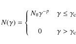
NIR spectroscopy has shown that a power-law fit,
![]() (where
(where ![]() ,
,
![]() and
and ![]() are
the flux, frequency and spectral index respectively), can describe
the observed spectrum of NIR flares. Although all the observations
agree with the fact that NIR flares show a soft spectrum
(
are
the flux, frequency and spectral index respectively), can describe
the observed spectrum of NIR flares. Although all the observations
agree with the fact that NIR flares show a soft spectrum
(![]() ), the value of the spectral index is still not well
determined. The first NIR spectroscopy observations in July 2004
(Eckart et al. 2004) proposed the
), the value of the spectral index is still not well
determined. The first NIR spectroscopy observations in July 2004
(Eckart et al. 2004) proposed the ![]() value to be
value to be
![]() during the peak of the flare. In 2006, Gillessen et al. (2006)
observed a correlation between flux and spectral index in their
observations. However, recent observations by Hornstein et al.
(2007) are consistent with a constant spectral index,
during the peak of the flare. In 2006, Gillessen et al. (2006)
observed a correlation between flux and spectral index in their
observations. However, recent observations by Hornstein et al.
(2007) are consistent with a constant spectral index,
![]() .
.
The actual value of the spectral index shows its importance in the
modeling of the physical process responsible for the flaring
emission. Some current models (Melia et al. 2001; Liu et al. 2006;
Yuan et al. 2007), predict that during flares a fraction of
electrons near the event horizon of the black hole are accelerated.
This can be described in the simplest form by a power law
distribution in the energy of radiating electrons,
![]() where
where
![]() and pare the energy distribution function of electrons, normalizing
constant, Lorentz factor of the electrons and the energy spectral
index respectively. For high values of
and pare the energy distribution function of electrons, normalizing
constant, Lorentz factor of the electrons and the energy spectral
index respectively. For high values of ![]() one will need a
sharp cut-off to the energy spectrum of electrons (
one will need a
sharp cut-off to the energy spectrum of electrons (
![]() ), while
a lower value of
), while
a lower value of ![]() (
(
![]() )
allows for a relatively
milder distribution in the energy of electrons. Liu et al. (2006)
have shown that simultaneous NIR and X-ray spectral measurements can
constrain the parameters of the emitting region well.
)
allows for a relatively
milder distribution in the energy of electrons. Liu et al. (2006)
have shown that simultaneous NIR and X-ray spectral measurements can
constrain the parameters of the emitting region well.
Before describing the details of our simulations, here we discuss
how the existing observations limit the possible range of free
parameters. Observationally it is proven that in the Sgr A* spectrum
a turn-over frequency in the sub-millimeter to NIR
range exists. By using the turn-over frequency relation,
![]() GHz, one can put an upper limit on
GHz, one can put an upper limit on
![]() ,
where B is the magnetic field strength in Gauss.
Here we have used
,
where B is the magnetic field strength in Gauss.
Here we have used
![]() and B=60G which give the best
fit to the NIR/X-ray models that already exist (Liu et al. 2006;
Eckart et al. 2008a).
and B=60G which give the best
fit to the NIR/X-ray models that already exist (Liu et al. 2006;
Eckart et al. 2008a).
In our simulations we first considered a scenario in which the main flare is caused by a local perturbation of intensity close to the marginally stable orbit (via magnetic reconnections, stochastic acceleration of electrons due to MHD waves, magneto rotational instabilities (MRI) etc.). These instabilities spread out and produce a temporary bright torus around the black hole. In this scenario, the mentioned variabilities are mainly due to relativistic flux modulations caused by the presence of an azimuthal asymmetry in the torus.
Simulations are dealing with two important velocities: radial
(![]() )
and azimuthal (
)
and azimuthal (![]() ). The radial velocity can be
parameterized in the following way:
). The radial velocity can be
parameterized in the following way:
![]() which depends on the ratio of the stress to the magnetic field energy
density,
which depends on the ratio of the stress to the magnetic field energy
density, ![]() ,
and the ratio of the magnetic energy density
to the thermal pressure,
,
and the ratio of the magnetic energy density
to the thermal pressure,
![]() (Melia 2007). The use of the typical
values of
(Melia 2007). The use of the typical
values of
![]() and
and ![]() from MHD simulations give us an
estimation (
from MHD simulations give us an
estimation (
![]() ). This leads to a radial
velocity of the order of
). This leads to a radial
velocity of the order of
![]() .
For
the azimuthal velocity, we assumed that above the marginally stable
orbit the plasma is in a Keplerian orbit,
.
For
the azimuthal velocity, we assumed that above the marginally stable
orbit the plasma is in a Keplerian orbit,
![]() where
where
![]() ,
and inside the plunging region the matter
experiences free fall with the same angular momentum as at the
marginally stable orbit.
,
and inside the plunging region the matter
experiences free fall with the same angular momentum as at the
marginally stable orbit.
Furthermore, two important time scales are at work: heating and
cooling time scales. The heating time scale strongly depends on the
physical processes which act as the engine of the whole event (MHD
instabilities, magnetic reconnections etc.), and one can just put an
observational constraint on that according to the averaged observed
rise time of the events (
![]() min). Cooling time is
mainly controlled by the Keplerian shearing and synchrotron loss
time,
min). Cooling time is
mainly controlled by the Keplerian shearing and synchrotron loss
time,
![]() min,
where B must be set in Gauss and
min,
where B must be set in Gauss and ![]() is in GHz.
is in GHz.
3.2 Hot spot model and fluctuations of the inner parts of the accretion disk
Since all these physical processes happen very close to the black hole and in a very strong gravitational regime, we must take into account the effects of curved space-time. To simulate the changes in paths and polarization properties of photons from the emitting electrons to the observer at infinity, we have used the KY ray-tracing code (Karas et al. 1992; Dovciak et al. 2004). KY is able to calculate all the effects of GR, like light bending and changes in the emission angle, changes in the polarization angle of photons, gravitational lensing and redshift, Doppler boosting (since matter inside the accretion disk is in orbit) and frame dragging (in case of Kerr black holes) in a thin disk approximation. In the geometrical optics approximation, photons follow null geodesics, and their propagation is not affected by spin-spin interaction with a rotating BH (Mashoon 1973). This means that wave fronts do not depend on the photon polarization, and so the ray tracing through the curved space-time is adequate to determine the observed signals. Since our analysis is focused on high frequency regimes, we have mainly ignored radiative transfer effects.
![\begin{figure}
\par\includegraphics[width=8cm,clip]{12473f14.eps}
\end{figure}](/articles/aa/full_html/2010/02/aa12473-09/img135.png)
|
Figure 14:
The geometry we considered in our emission model. The
accretion disk around the black hole lies on the
|
| Open with DEXTER | |
To make KY work, we must initialize the properties of radiated
photons at each point of the emitting region. The straightforward
way is to define the intrinsic emission of each point in the context
of the Stokes parameters. For the flux densities (mJy) and
source sizes (![]() as) of Sgr A*, optically thick synchrotron
emission in the NIR can safely be disregarded (see the discussion in
Eckart et al. 2009). Since in this report we focus only on the modeling
of the NIR flares, it is sufficient to pick up a model for the
energy distribution of non-thermal electrons, radiating in an
optically thin regime:
as) of Sgr A*, optically thick synchrotron
emission in the NIR can safely be disregarded (see the discussion in
Eckart et al. 2009). Since in this report we focus only on the modeling
of the NIR flares, it is sufficient to pick up a model for the
energy distribution of non-thermal electrons, radiating in an
optically thin regime:
which leads to the formulae for polarized emission:
| (8) | ||
| (9) | ||
| (10) | ||
| (11) |
where n,
|
(12) |
where we have picked the disk co-moving frame as the reference, so that the normal to the disk,
|
(13) |
where v is the four-velocity of matter in the disc.
|
(14) |
Having all the needed information at hand, by fixing free parameters like the spatial density distribution of the emitting electrons, magnetic field strength, flux spectral index, and the global configuration of the magnetic field, one can simulate the expected images that a distant observer will measure for different possible inclinations with respect to the black hole/accretion disk system. Here we will show how compact azimuthal anomalies inside a uniform density distribution of the emitting plasma can reproduce the observed behavior of Sgr A* in high frequency regimes.
The synchrotron cooling time at NIR frequencies is only of the order
of a few minutes, which is significantly shorter than the time scale
of the observed flares. One way that a spot can survive long enough
to be responsible for the observed
![]() time flux
modulations is that a SSC mechanism up-scatters the sub-mm seed
photons to the NIR and X-ray frequencies (Eckart et al. 2006a-c,
2008a). The other possibility is that the heating time of the orbiting NIR
component is related to the rise time of the main flare,
time flux
modulations is that a SSC mechanism up-scatters the sub-mm seed
photons to the NIR and X-ray frequencies (Eckart et al. 2006a-c,
2008a). The other possibility is that the heating time of the orbiting NIR
component is related to the rise time of the main flare,
![]() where the emissivity profile of the emitting
component follows
where the emissivity profile of the emitting
component follows
![]() .
.
The above discussion demonstrates that it is essential to consider
the gravitational shearing time scale as a variable in the
simulations. We have implemented this effect in our modeling by
introducing a dimensionless characteristic shearing time scale:
|
(15) |
where for the initial spatial distribution of the relativistic electrons we have used a spherical Gaussian distribution with its maximum being located at the radius
3.3 Results of the modeling
Figure 15 shows how a hot spot
is created and evolves in time for three different values of
![]() .
A comparison between the rows shows how pure Keplerian
shearing disrupts the initial shape of the spot and produces an
elongated spiral shape. Figure 16 shows the
apparent images of a spot with a mild shearing environment
(
.
A comparison between the rows shows how pure Keplerian
shearing disrupts the initial shape of the spot and produces an
elongated spiral shape. Figure 16 shows the
apparent images of a spot with a mild shearing environment
(
![]() )
for three different inclination angles. When we
look face-on at the event (
)
for three different inclination angles. When we
look face-on at the event (
![]() ), there are no
modulations by the relativistic effects. For higher inclination
angles (
), there are no
modulations by the relativistic effects. For higher inclination
angles (
![]() )
lensing and
boosting effects play major roles in the observed flux modulations.
Specially for high inclinations one can see how an Einstein arc
develops when the spot passes behind the black hole and how photons
coming from the accretion disk are blue-shifted on the left hand side of the
image according to Doppler boosting. This set-up allows us to
simulate light curves for a wide range of possible free parameters,
mainly by covering the range of all possible inclinations and
spins of the black hole. Figure 17 shows examples of light curves for different
values of inclination and shearing time scale.
)
lensing and
boosting effects play major roles in the observed flux modulations.
Specially for high inclinations one can see how an Einstein arc
develops when the spot passes behind the black hole and how photons
coming from the accretion disk are blue-shifted on the left hand side of the
image according to Doppler boosting. This set-up allows us to
simulate light curves for a wide range of possible free parameters,
mainly by covering the range of all possible inclinations and
spins of the black hole. Figure 17 shows examples of light curves for different
values of inclination and shearing time scale.
![\begin{figure}
{\includegraphics[width=18cm,clip]{12473f15.eps} }\end{figure}](/articles/aa/full_html/2010/02/aa12473-09/img170.png)
|
Figure 15:
Snapshots of orbiting anomalies inside the accretion disk
as they appear to a distant observer looking along a line of sight
inclined by |
| Open with DEXTER | |
![\begin{figure}
{\includegraphics[width=17.5cm,clip]{12473f16.eps} }
\end{figure}](/articles/aa/full_html/2010/02/aa12473-09/img171.png)
|
Figure 16:
Snapshots of an orbiting anomaly inside the accretion disk
as it appears to a distant
observer looking along a line of sight inclined by |
| Open with DEXTER | |
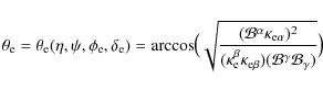
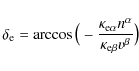
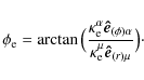
3.3.1 Pattern recognition analysis: signatures of lensing effects
Figure 18 shows the typical magnification of flux, polarization angle and degree of an orbiting spot emission as a function of time. Here we showed the spots located at different distances from the black hole. These plots indicate the typical behavior of light curves when the strong gravitational regime is prominent and the strong lensing and boosting is happening. As one can see, the sweep in the polarization angle precedes the peak in flux magnification, while the peak of the degree of polarization follows the magnification peak (see Broderick & Loeb 2006, for a detailed discussion). Figure 19 shows more clearly this typical behavior according to the position of the corresponding cross-correlation's peaks. It is particularly apparent that even with changing the position of the emitting source with respect to the black hole this effect remains more or less the same.
![\begin{figure}
{\includegraphics[width=8.5cm,clip]{12473f17.eps} }
\end{figure}](/articles/aa/full_html/2010/02/aa12473-09/img172.png)
|
Figure 17: Flux modulations of an evolving perturbation close to the marginally stable orbit of a Kerr black hole with spin parameter of 0.5. The light curves show how different values of shearing parameter and inclination affects the resultant light curve. |
| Open with DEXTER | |
![\begin{figure}
{\includegraphics[width=8cm,clip]{12473f18.eps} }
\vspace*{3mm}
\end{figure}](/articles/aa/full_html/2010/02/aa12473-09/img173.png)
|
Figure 18:
Flux modulation ( top), changes in polarization
angle ( middle) and degree ( bottom) for a spot on a circular orbit at
|
| Open with DEXTER | |
This constant behavior encouraged us to check whether or not this type of pattern is manifested in our NIR light curves of Sgr A*. For this purpose we used a simple pattern recognition algorithm mainly via a multiplication of different cross correlation functions. Similar pattern recognition algorithms are used to identify gravitational wave signals from noisy data (Pappa et al. 2003; Goggin 2008).
We derived a final pattern recognition coefficient product by multiplying two cross correlation functions
(namely
![]() and
and
![]() )
as below:
)
as below:
By applying this procedure for the cross correlation functions between the observed flux and the theoretical magnification light curve (
Figure 21 shows the result of our pattern
recognition analysis for the polarized flare events discussed in
this paper. In order to estimate how significant the peaks in the
![]() function are, we have repeated the same analysis for 104 random red noise light curves simulated with the same method
mentioned in Sect. 2.2.2. In all but one case the patterns shown in
Fig. 21 can be identified at the
function are, we have repeated the same analysis for 104 random red noise light curves simulated with the same method
mentioned in Sect. 2.2.2. In all but one case the patterns shown in
Fig. 21 can be identified at the
![]() to
to
![]() level. This shows that strong lensing patterns are
significantly manifested in our sample of NIR light curves.
The strong lensing pattern detected is a further indicator for the existence of
a (clumpy) accretion disk around Sgr A*.
level. This shows that strong lensing patterns are
significantly manifested in our sample of NIR light curves.
The strong lensing pattern detected is a further indicator for the existence of
a (clumpy) accretion disk around Sgr A*.
3.3.2 A spotted accretion disk?
Figure 22 shows a selected 100 min window of the
resultant light curves of the flux density, polarization degree and
angle for a spot with constant shape (
![]() ), orbiting
around a Kerr black hole (a=0.5) close to its marginally stable
orbit (
), orbiting
around a Kerr black hole (a=0.5) close to its marginally stable
orbit (
![]() ). The line of sight is inclined by 60 degrees (
). The line of sight is inclined by 60 degrees (
![]() ). Gaussian white noise has been added to the
simulated data in order to make the comparison of the periodicity
and cross correlation with corresponding observational results
easier. The level of the noise and the average error bars have been
set from the average rms of the corresponding observed light curves. The
surface brightness of the components follows a profile similar to
). Gaussian white noise has been added to the
simulated data in order to make the comparison of the periodicity
and cross correlation with corresponding observational results
easier. The level of the noise and the average error bars have been
set from the average rms of the corresponding observed light curves. The
surface brightness of the components follows a profile similar to
![]() with
with ![]() .
The maximum degree of polarization
which can be achieved via synchrotron mechanism is around 70%.
Since any kind of deviation from the ideal isotropic distribution of
electrons around the magnetic field lines will suppress the degree
of linear polarization, we set the initial value for the radiation
from the spot to be 50%. We assumed that the photons originating
from the non-flaring part of the accretion disk
are weakly polarized (
.
The maximum degree of polarization
which can be achieved via synchrotron mechanism is around 70%.
Since any kind of deviation from the ideal isotropic distribution of
electrons around the magnetic field lines will suppress the degree
of linear polarization, we set the initial value for the radiation
from the spot to be 50%. We assumed that the photons originating
from the non-flaring part of the accretion disk
are weakly polarized (![]() ), since the main population of its NIR photons have
thermal origin and relativistic electrons are randomly distributed
around the magnetic field lines.
), since the main population of its NIR photons have
thermal origin and relativistic electrons are randomly distributed
around the magnetic field lines.
Figure 23 shows the result from
autocorrelation and Lomb-Scargle analysis (similar to Figs. 3 and 5), and Fig. 24 shows the
results of the cross correlation analysis (similar to Fig. 8). The peaks close to the 0 min time-lag are of special
interest since they have the least dependency on the choice of free
parameters and are mainly related to the basic idea that the flux
modulations are caused by relativistic effects. Figures 23 and 24 show that an orbiting
spot is able to produce the same cross correlation pattern observed
in our sample, but the orbital frequency of the spot will be detected
to be mainly a quasi-periodical signal. The corresponding correlation functions of the 30 july
2005 observation are over-plotted in Fig. 24 for a
better comparison. The main peak close to ![]() coincides very
well for both observation and simulated cross-correlations.
coincides very
well for both observation and simulated cross-correlations.
Furthermore, we have simulated a spotted accretion disk. In
this case spots are born, evolve and finally fade away as a function
of time. These anomalies are distributed in the inner part of the
accretion disk in a belt between
![]() .
Radial and
azimuthal distribution of the anomalies are completely random and
their distribution in time follows a simple Poisson point process
(see Pechácek et al. 2008).
.
Radial and
azimuthal distribution of the anomalies are completely random and
their distribution in time follows a simple Poisson point process
(see Pechácek et al. 2008).
Figure 25 shows the snapshots of the spotted disk scenario as viewed by a distant observer from different inclination angles. The resulting magnification and polarimetric light curves are depicted in Fig. 26. White noise is added to all light curves in order to make the comparison between ZDCF and Lomb-Scargle results with the corresponding observational results easier. As can be seen in Fig. 27 the random distribution of the spots strongly suppresses the periodic signal in the Lomb-Scargle periodogram, while the cross correlation between the magnification and the changes in the polarized flux still carries a significant signal from the modulations influenced by strong gravity (Fig. 28). As a conclusion one can say that a general relativistic simulation of turbulences in the inner parts of an accretion disk resembles the observed behavior of Sgr A* very well.
One must note that for the simulated data, we have chosen typical values for spin and inclination (consistent with previous results by Eckart et al. 2006b and Meyer et al. 2006a,b), not trying to fit the actual data. As we can see, the data analysis and simulations show that even if there does exist a low-level activity physical process in Sgr A* which can be explained as random red-noise, the kind of observed correlations between the flux and polarization data cannot be produced via a completely random process (without taking into account relativistic effects). Actually, the similarity between Figs. 24 and 28 and what is already observed in at least three different Sgr A* flares (Figs. 5 and 8), supports the idea of orbiting matter around the galactic super-massive black hole.
![\begin{figure}
{\includegraphics[width=8cm,clip]{12473f19.eps} }\vspace*{7mm}
\end{figure}](/articles/aa/full_html/2010/02/aa12473-09/img184.png)
|
Figure 19:
Cross correlation between the changes in flux and
polarization angle ( top), and flux and polarization degree ( bottom)
for spot circular orbits at
|
| Open with DEXTER | |
3.4 Alternative models
As mentioned before, the strength of ZDCF's peaks in Fig. 3 seems to be correlated with the brightness of flare
events. This dependency on the brightness of the flares and also
the shape of the resulting ZDCFs are very similar to the expected
autocorrelation if the flux variations originate from geometric
``light echoes'' (Bursa et al. 2007; Fukumura et al. 2009). The
expected periodicities from these models are different from the ones
observed here, but their very close similarity keeps this issue open to
future discussions. If a more detailed modeling of random flares
happening at a distance from the black hole can show a possible
![]() min QPO, then the light curve observed on 15 and 17 may 2007 could be the first observation of second images created
from separated photon ``bunches'' (Fukumura 2009).
min QPO, then the light curve observed on 15 and 17 may 2007 could be the first observation of second images created
from separated photon ``bunches'' (Fukumura 2009).
Furthermore, shocks in relativistic jets can produce a correlated total flux and polarized intensity. There is a possibility that under special circumstances (e.g. special inclination, special magnetic field configuration etc.) a (episodic) relativistic outflow could produce the same correlation and pattern we have discovered in our observations.
4 Geometry of the emitting region
In this section we discuss the basic assumption of the existence of an azimuthal asymmetry in the accretion flow of Sgr A*. Recently, Falanga et al. (2007) and Karas et al. (2007) discussed that a global spiral pattern of disturbance, with an orbiting speed not directly associated with the underlying Keplerian velocity, can fit the observed NIR and X-ray modulations of Sgr A*. Their model has been used to fit the observed X-ray flare on 31 august 2004 (Falanga et al. 2007). Here we will show how a combination of polarimetric observations and the next generation of VLTI measurements can reveal the geometry of the emitting region of these high frequency photons.
![\begin{figure}
{\includegraphics[width=17.5cm,clip]{12473f20.eps} }
\end{figure}](/articles/aa/full_html/2010/02/aa12473-09/img187.png)
|
Figure 20:
A sketch showing how the pattern recognition
coefficient ( |
| Open with DEXTER | |
In order to reproduce the same density profile in the inner part of
the disk, we have used a spiral pattern, characterized by the
emissivity function given below:
|
(17) |
while the power-law index,
![\begin{figure}
{\includegraphics[width=17.5cm,clip]{12473f21.eps} }
\end{figure}](/articles/aa/full_html/2010/02/aa12473-09/img193.png)
|
Figure 21:
Pattern recognition coefficients as a function of
time for our sample of observations (13 June 2004 a); 30 July 2005
b); 1 June 2006 c); 15 May 2007 d); 17 May 2007 e) and 28 May
2008 f)). Dotted lines show the median (red), |
| Open with DEXTER | |
![\begin{figure}
{\includegraphics[width=8cm,clip]{12473f22.eps} }\end{figure}](/articles/aa/full_html/2010/02/aa12473-09/img194.png)
|
Figure 22:
A selected 100 min window of the white noise added
simulated light curves of an orbiting spot plus a temporary
variability in the accretion disk. The flux density is presented in
arbitrary units ( top). Middle and bottom panels show the changes in
the angle (degree) of polarization. The spin of the black hole is
set to be a=0.5 and the inclination fixed on
|
| Open with DEXTER | |
![\begin{figure}
{\includegraphics[width=8.5cm,clip]{12473f23.eps} }\end{figure}](/articles/aa/full_html/2010/02/aa12473-09/img195.png)
|
Figure 23:
Same as Figs. 3 and 5 for the
simulated light curves of Fig. 22. The top shows the
autocorrelation of the flux while the bottom shows the Lomb-Scargle
periodogram. The colored regions indicate the position of the
peaks corresponding to the
|
| Open with DEXTER | |
The main idea in our simulations is to include the polarimetric
radiation transfer in curved space-time, which provides the
possibility to compare the behavior of different geometrical
configurations. It seems that even though both of these geometrical
set-ups (spiral shape or compact spot) show the same behavior in
flux, the observed polarized flux will behave significantly
different. In order to reduce the effects of our specific
assumptions about the emission process and magnify the signatures
which result only from different geometrical structures, we have
chosen a toy model for the initial polarized emission:
![]() .
Figure 30 shows that the spiral
pattern is unable to produce strong changes in the polarization angle,
while a compact azimuthal source produces a highly variable
polarization angle. Due to abberation,
photons that come from different parts of the
disk are polarized differently, even for Schwarzschild black
holes. For the Kerr case, the rotation of the polarization vector
will be added because of gravitational frame dragging. The
dependency of these changes on the position of the emitted photon
is depicted in Fig. 31. The top panel of Fig. 31 shows how the polarization vector of the emitted photons
will be rotated due to the strong gravity of the central black hole.
As one can see, there is a clear knot visible in
this contour graph. If the radiating source passes through this
knot, the observed polarization angle will swing dramatically (for a
detailed discussion see Dovciak et al. 2008). As the bottom
panel of Fig. 31 shows, when a compact azimuthal source
orbiting around the black hole is close to its marginally stable orbit,
this nod will be passed. The amount of change in the polarization
angle depends on the compactness of the source, its position
relative to the black hole, the inclination of the observer and the
spin of the black hole. On the other hand, if the flare-emitting
region is a deformed pattern extending in both radial and azimuthal
directions, the swing in the polarization angle will not be strong.
It is because of the fact that in each point of the light curve the
polarization angle is the average of photons that come from
different parts of the disk and have a different polarization angle
(Fig. 31). As a result, the swings in the angles cancel each
other out, and no significant swing will be observed.
.
Figure 30 shows that the spiral
pattern is unable to produce strong changes in the polarization angle,
while a compact azimuthal source produces a highly variable
polarization angle. Due to abberation,
photons that come from different parts of the
disk are polarized differently, even for Schwarzschild black
holes. For the Kerr case, the rotation of the polarization vector
will be added because of gravitational frame dragging. The
dependency of these changes on the position of the emitted photon
is depicted in Fig. 31. The top panel of Fig. 31 shows how the polarization vector of the emitted photons
will be rotated due to the strong gravity of the central black hole.
As one can see, there is a clear knot visible in
this contour graph. If the radiating source passes through this
knot, the observed polarization angle will swing dramatically (for a
detailed discussion see Dovciak et al. 2008). As the bottom
panel of Fig. 31 shows, when a compact azimuthal source
orbiting around the black hole is close to its marginally stable orbit,
this nod will be passed. The amount of change in the polarization
angle depends on the compactness of the source, its position
relative to the black hole, the inclination of the observer and the
spin of the black hole. On the other hand, if the flare-emitting
region is a deformed pattern extending in both radial and azimuthal
directions, the swing in the polarization angle will not be strong.
It is because of the fact that in each point of the light curve the
polarization angle is the average of photons that come from
different parts of the disk and have a different polarization angle
(Fig. 31). As a result, the swings in the angles cancel each
other out, and no significant swing will be observed.
![\begin{figure}
{\includegraphics[width=8.5cm,clip]{12473f24.eps} }\end{figure}](/articles/aa/full_html/2010/02/aa12473-09/img197.png)
|
Figure 24: Top ( bottom): Cross correlation between the total flux and polarization angle (degree) of the simulated light curve (Fig. 22). Dotted lines indicate the corresponding cross correlation functions for the 30 july 2005 flare as the case most similar to the predictions of the hot spot model. |
| Open with DEXTER | |
The presence of changes in the degree of the NIR polarization and the swings in the observed polarization angle simultaneous to the flux magnifications supports the idea that the geometrical shape of the sources is dominated by compact azimuthal asymmetries rather than by radially extended spiral patterns (see also discussion in Sect. 6 about the differences in the centroid motions of these two types of geometries). Here we must note that as Tagger et al. (2006) have mentioned, a second initial configuration was used in their simulations (simulation no. 2, Tagger et al. 2006). In that set-up, a clump of matter starts spiraling towards the black hole and produces the spiral Rossby wave. There, the ratio of the surface brightness between the hot core moving radially inward and the tail which is produced plays a critical role in the resulting light curves. If the hot core is dramatically brighter than the tail, there is no practical difference between this scenario and the orbiting spot model. For a complete polarization study of Rossby wave instabilities, one needs simulated profiles of MHD surface densities as a function of time, which is beyond the scope of this paper.
5 Magnetic field structure and geometrical orientation of the system
In our simulations the structure of the magnetic field lines
according to the black hole/accretion disk system can be controlled
by a set of parameters [![]() ,
,
![]() ]. Of special interest are two
extreme configurations in which the envelope of the accelerated
electrons is located inside the accretion disk with a global
toroidal magnetic field (model I: [
]. Of special interest are two
extreme configurations in which the envelope of the accelerated
electrons is located inside the accretion disk with a global
toroidal magnetic field (model I: [
![]() ]) or inside a region with magnetic field lines
perpendicular to the disk (model II: [
]) or inside a region with magnetic field lines
perpendicular to the disk (model II: [
![]() ]). The
latter can be interpreted as the spot being located at the tip of a
jet with magnetic field lines aligned parallel to its symmetry axis
(see Fig. 32).
]). The
latter can be interpreted as the spot being located at the tip of a
jet with magnetic field lines aligned parallel to its symmetry axis
(see Fig. 32).
We assumed that the magnetic field inside the accretion disk is dominated by the toroidal component. This structure is compatible with the results of several MHD simulations (Hawley & Balbus 1991; Hirose et al. 2004; De Villiers et al. 2003). However, in our case it is not clear if the cloud of accelerated electrons is located inside the accretion disk, somewhere above it in the corona, or even inside the tip of a possible short jet/wind. In fact, there is a possibility that a source structure in which an accretion disk is associated with a short jet/collimated outflow can explain the multi-wavelength behavior of Sgr A* (Markoff et al. 2001; Yuan et al. 2002; Eckart et al. 2005, 2006a, 2008a-c). Here we discuss how different orientations of the magnetic field lines inside the emitting region affect the resultant physical parameters that one can extract via fitting the model to the observed data.
The KY code allows us to simulate light curves for a wide range of
free parameters, so one can fit the model parameters to the actual
observed data (Meyer et al. 2006a,b, 2007; Eckart et al. 2006a,b,
2008). For this purpose, simulations have been carried out, as they
cover a wide enough range of possible inclinations (
![]() ), the initial degree of linear polarization
(
), the initial degree of linear polarization
(
![]() ), possible combinations of
), possible combinations of ![]() and
and
![]() ,
and different orientations of the whole system on the sky
(
,
and different orientations of the whole system on the sky
(
![]() ). Here
). Here ![]() defines the
direction of the normal to the accretion disk projected on the sky.
The spot has an initial radius of
defines the
direction of the normal to the accretion disk projected on the sky.
The spot has an initial radius of
![]() and orbits very closely to
the marginally stable orbit of a Kerr black hole (a=0.5). The
dimensionless shearing time scale is fixed to be 2.0
(
and orbits very closely to
the marginally stable orbit of a Kerr black hole (a=0.5). The
dimensionless shearing time scale is fixed to be 2.0
(
![]() ), and the ratio of the surface brightness of the
spot to the torus is set to five. We have chosen these values according
to existing results of several fits to the NIR flares (Meyer et al. 2006a,b; Eckart et al. 2006b, 2008).
), and the ratio of the surface brightness of the
spot to the torus is set to five. We have chosen these values according
to existing results of several fits to the NIR flares (Meyer et al. 2006a,b; Eckart et al. 2006b, 2008).
As a first step, we focus on model I (
![]() ). In order to find the fit with best
). In order to find the fit with best
![]() we have carried out a grid search in a
(
we have carried out a grid search in a
(
![]() )
parameter space. The steps for i,
)
parameter space. The steps for i, ![]() and
and
![]() have been chosen to be
have been chosen to be ![]() ,
,
![]() and
and ![]() ,
respectively. The least
,
respectively. The least
![]() value was achieved for a high
inclination angle (
value was achieved for a high
inclination angle (
![]() ),
),
![]() and highly
polarized source (
and highly
polarized source (
![]() )
(see Fig. 33 and Table 2).
The grid search has been performed
on
)
(see Fig. 33 and Table 2).
The grid search has been performed
on
![]() ,
i and
,
i and ![]() for the models I and II. The free
parameters in model III are
for the models I and II. The free
parameters in model III are
![]() ,
i,
,
i, ![]() and
and ![]() .
Figure 34 shows the resultant possible range for the
orientation of the correlated outflow/wind in this scenario.
Interestingly, the observed position of the mini-cavity lies well
within this interval. Muzic et al. (2007) have shown how a
collimated outflow from the position of Sgr A* can describe the
observed motion of filamentary structures and the mini-cavity,
according to their observations in the NIR L'-band. This
observational evidence supports the idea that the NIR flares
actually originate in accelerated electrons within an accretion
disk.
.
Figure 34 shows the resultant possible range for the
orientation of the correlated outflow/wind in this scenario.
Interestingly, the observed position of the mini-cavity lies well
within this interval. Muzic et al. (2007) have shown how a
collimated outflow from the position of Sgr A* can describe the
observed motion of filamentary structures and the mini-cavity,
according to their observations in the NIR L'-band. This
observational evidence supports the idea that the NIR flares
actually originate in accelerated electrons within an accretion
disk.
![\begin{figure}
{\includegraphics[width=17.5cm,clip]{12473f25.eps} }
\end{figure}](/articles/aa/full_html/2010/02/aa12473-09/img211.png)
|
Figure 25:
Same as Fig. 16 for the
multi-component scenario. The observer's inclination is set to |
| Open with DEXTER | |
For model II ([
![]() ]), the envelope of relativistic
electrons has been located somewhere in the bottom of an outflow.
The least
]), the envelope of relativistic
electrons has been located somewhere in the bottom of an outflow.
The least
![]() achieved for this model and related
parameters are presented in Table 2. Possible directions of this jet
structure are depicted in Fig. 34. As one can see,
achieved for this model and related
parameters are presented in Table 2. Possible directions of this jet
structure are depicted in Fig. 34. As one can see,
![]() values and observational facts support the idea
that the NIR photons originate in the inner parts of an accretion
disk rather than in an outflow (Thorne 1994; Blandford 2001).
values and observational facts support the idea
that the NIR photons originate in the inner parts of an accretion
disk rather than in an outflow (Thorne 1994; Blandford 2001).
Table 2:
Final parameters resulting from the best
![]() fit
to the NIR flare observed on 30 july 2005.
fit
to the NIR flare observed on 30 july 2005.
One can also invert the question and try to constrain the magnetic
field structure of the emitting region by fixing the direction of
the outflow in the plane of the sky (model III). For this purpose, a
![]() search has been carried out, assuming that the
normal to the disk is fixed at
search has been carried out, assuming that the
normal to the disk is fixed at
![]() .
This is the
best value that can fit the observed position of the mini-cavity
(Muzic et al. 2007). By a good approximation, the best fit
is achieved for a toroidal magnetic field structure (see Table 2).
This shows that if any future observations reveal traces of an
outflow from Sgr A*, NIR polarimetry could be used as a tool to
constrain its magnetic field structure.
.
This is the
best value that can fit the observed position of the mini-cavity
(Muzic et al. 2007). By a good approximation, the best fit
is achieved for a toroidal magnetic field structure (see Table 2).
This shows that if any future observations reveal traces of an
outflow from Sgr A*, NIR polarimetry could be used as a tool to
constrain its magnetic field structure.
![\begin{figure}
{\includegraphics[width=8.5cm,clip]{12473f26.eps} }
\end{figure}](/articles/aa/full_html/2010/02/aa12473-09/img229.png)
|
Figure 26: Same as Fig. 22 but a selected 200 min-window of the multi component scenario. |
| Open with DEXTER | |
![\begin{figure}
{\includegraphics[width=8.5cm,clip]{12473f27.eps} }\end{figure}](/articles/aa/full_html/2010/02/aa12473-09/img230.png)
|
Figure 27: Same as Figs. 23 for the multi-component scenario (Fig. 26). |
| Open with DEXTER | |
![\begin{figure}
{\includegraphics[width=8.5cm,clip]{12473f28.eps} }
\end{figure}](/articles/aa/full_html/2010/02/aa12473-09/img231.png)
|
Figure 28: Same as Figs. 24 for the multi-component scenario (Fig. 26). |
| Open with DEXTER | |
6 Next generation of NIR interferometry
According to its proximity, Sgr A* is known as the best candidate
for studying the details of physical processes on the event horizon
scales (Falcke et al. 2000; Bromley et al. 2001). VLT and Keck
telescopes have already achieved angular resolutions as high as
40 mas in their imaging mode (Genzel et al. 2003; Eckart et al. 2004,
2006a,b; Ghez et al. 2005). In interferometric mode these telescopes
can observe with resolutions of the order of only a few mas. The
next generation of VLT Interferometer instrument, namely GRAVITY,
would be able to achieve resolutions of the order of 10 ![]() as in
its phase-reference tracking mode. GRAVITY will try to measure
the position of the lumicenter
of the flares with respect to a reference source. For such a measurement
the 1
as in
its phase-reference tracking mode. GRAVITY will try to measure
the position of the lumicenter
of the flares with respect to a reference source. For such a measurement
the 1![]() uncertainty is
uncertainty is ![]()
![]() as
with an integration time of five minutes on an assumed K=15 pointsource.
The real necessary integration time for that precision is of course directly dependent on the magnitude of the flare.
This resolution is high enough to track the
centroid motion of NIR images of Sgr A* with a resolution of the
order of one Schwarzschild radius (Eisenhauer et al. 2005, 2008;
Gillessen et al. 2006). These unique
features make the next generation of VLTI a perfect instrument for
high accuracy astrometry of the matter around Sgr A*. Recently,
Doeleman et al. (2008) proposed a VLBI configuration with a high
enough time resolution to possibly track the centroid motion
of sub-mm images of Sgr A* with even higher angular resolution. In
this section we present the results of our study on centroid motion
of the NIR image of Sgr A*.
as
with an integration time of five minutes on an assumed K=15 pointsource.
The real necessary integration time for that precision is of course directly dependent on the magnitude of the flare.
This resolution is high enough to track the
centroid motion of NIR images of Sgr A* with a resolution of the
order of one Schwarzschild radius (Eisenhauer et al. 2005, 2008;
Gillessen et al. 2006). These unique
features make the next generation of VLTI a perfect instrument for
high accuracy astrometry of the matter around Sgr A*. Recently,
Doeleman et al. (2008) proposed a VLBI configuration with a high
enough time resolution to possibly track the centroid motion
of sub-mm images of Sgr A* with even higher angular resolution. In
this section we present the results of our study on centroid motion
of the NIR image of Sgr A*.
Some predictions of the centroid motions related to the hot spot
model have already been studied by several authors (Broderick & Loeb 2006a,b; Paumard et al. 2006; Zamaninasab et al. 2008b; Hamaus et al. 2009). In previous works it has been mainly assumed that the
spots preserve their shape in time. This assumption has been
based mostly on the presence of strong magnetic field lines or ``unknown
mechanisms'' (Hamaus et al. 2009). We will show here that it
is actually very crucial that the effects of gravitational shearing inside
the accretion disk are taken into account, since the predicted
results can change dramatically. The other very important fact to
be considered in the simulations is due to the NIR photons which
come from the body of the accretion disk and confuse with the spot's
emission. Since GRAVITY can only achieve its 10 ![]() as resolution in
the phase-reference tracking mode and not in the imaging mode, even
a constant confusion from the (thermal) electrons inside the
accretion disk can not be reduced.
as resolution in
the phase-reference tracking mode and not in the imaging mode, even
a constant confusion from the (thermal) electrons inside the
accretion disk can not be reduced.
Figure 35 represents how these two
parameters mentioned can affect the expected centroid tracks and may present a
complication in detecting the plasma structure close to the event
horizon of Sgr A*. The simulated paths in Fig. 35
belong to a configuration where the observer is aligned
approximately face-on (
![]() ). This is the inclination
in which the clearest wobbling of the centroid is expected to be
seen. Figure 35a shows that the position wanders of
the center of the images are large enough to be detected easily if
GRAVITY could achieve its five minutes time-resolution (simulated
points). Panels b and c in Fig. 35 show how
gravitational shearing changes the centroid track. One
can see in particular that in the case of pure Keplerian shearing the change in the
center is detectable for approximately only six points. The second
row (Fig. 35, panels d)-f)) shows the result of
the simulated tracks including the effect of confusion due to the
NIR photons coming from the inner parts of the accretion disk.
). This is the inclination
in which the clearest wobbling of the centroid is expected to be
seen. Figure 35a shows that the position wanders of
the center of the images are large enough to be detected easily if
GRAVITY could achieve its five minutes time-resolution (simulated
points). Panels b and c in Fig. 35 show how
gravitational shearing changes the centroid track. One
can see in particular that in the case of pure Keplerian shearing the change in the
center is detectable for approximately only six points. The second
row (Fig. 35, panels d)-f)) shows the result of
the simulated tracks including the effect of confusion due to the
NIR photons coming from the inner parts of the accretion disk.
Figure 36 shows the centroid paths of spots
orbiting in a mild shearing environment (
![]() )
for three
different inclinations (
)
for three
different inclinations (
![]() )
in
presence of confusion from the torus. Panel c shows that the
detection of any position wander becomes even more difficult in the
case of a shearing spot observed at high inclinations.
The bottom row in Fig. 36 shows the centroid motion
resultant from simulations including several emitting components
(Fig. 25).
The photons originated from the spot are highly polarized, while the
radiation from the torus is weakly polarized. This fact may lead us
to a solution for compensating for this kind of confusion.
Figure 37 shows how different the apparent images of the
flares are when they are observed in total flux or two
orthogonal polarized channels. One sees that the different centroid
paths can be revealed if GRAVITY could achieve its 10
)
in
presence of confusion from the torus. Panel c shows that the
detection of any position wander becomes even more difficult in the
case of a shearing spot observed at high inclinations.
The bottom row in Fig. 36 shows the centroid motion
resultant from simulations including several emitting components
(Fig. 25).
The photons originated from the spot are highly polarized, while the
radiation from the torus is weakly polarized. This fact may lead us
to a solution for compensating for this kind of confusion.
Figure 37 shows how different the apparent images of the
flares are when they are observed in total flux or two
orthogonal polarized channels. One sees that the different centroid
paths can be revealed if GRAVITY could achieve its 10 ![]() as
resolution in the polarimetry mode Fig. 38.
as
resolution in the polarimetry mode Fig. 38.
To summarize the results of this section, one can say that a non-detection of a position wander in NIR images of Sgr A* will not rule out a spotted disk scenario. On the other hand, a clear detection of such a position wander by GRAVITY would lead us to strongly favor the spot model and would open a new era in studying the physics of high gravitational regimes.
7 Summary and conclusion
We used a sample of NIR flares of Sgr A* observed in polarimetry mode to study the nature of the observed variability. Using the z-transformed discrete correlation function algorithm, we found a significant correlation between changes in the measured polarimetric data and total flux densities. This provides evidence that the variations probably originate from inner parts of an accretion disk while a strong gravity's effects are manifested inside them.
In order to obtain this information polarization data is indispensable since the corresponding signals are very difficult or even impossible to extract from simple total intensity light curves only (Do et al. 2008). The presence of significant signals from orbiting matter then calls for detailed modeling of the NIR polarized light curves in order to analyze the distribution of the emitting material and the magnetic field structure within the accretion disk (e.g. Eckart et al. 2006a, 2008a; Meyer et al. 2006a,b, 2007).
![\begin{figure}
\includegraphics[width=18cm,clip]{12473f29.eps}
\end{figure}](/articles/aa/full_html/2010/02/aa12473-09/img235.png)
|
Figure 29:
Snapshots of the orbiting spiral pattern as they appear to
a distant observer looking along a line of sight inclined by
|
| Open with DEXTER | |
![\begin{figure}
{\includegraphics[width=8.5cm,clip]{12473f30.eps} }
\end{figure}](/articles/aa/full_html/2010/02/aa12473-09/img236.png)
|
Figure 30:
Light curves of the normalized flux ( top, black) and
polarization angle ( bottom, blue) observed at infinity, obtained
form general relativistic modulations associated with a spiral
pattern ( left) or a compact spot ( right). Light curves are shown for
three different inclinations:
|
| Open with DEXTER | |
![\begin{figure}
{\includegraphics[width=6.87cm,clip]{12473f31.eps} }
\end{figure}](/articles/aa/full_html/2010/02/aa12473-09/img238.png)
|
Figure 31:
Top: Contour graphs showing the changes in the polarization
angle due to general relativistic effects. Bottom: Spatial
emissivity distribution of a compact hot spot. The observer's
inclination is
|
| Open with DEXTER | |
In addition, the pattern recognition algorithm we employed in this paper is an efficient tool to search for flare events that carry the signature of strong gravity in light curves which are significantly longer than the orbiting time scale over which such an event can typically occur. Other methods that make simultaneous use of the entire light curve (like e.g. the Lomb-Scargle algorithm) tend to dilute these signals and lower the possibility for significant detections dramatically (Do et al. 2008; Meyer et al. 2009).
In order to constrain the physical properties of the emitting region we employed a relativistic disk model with azimuthal over-densities of relativistic electrons. A combination of a synchrotron mechanism and relativistic amplifications allows us to fit the real observed data and make predictions about astrometric parameters of the accretion disk around Sgr A*. The modeled light curves show the same correlation between the flux and polarimetric data as the one deduced from observations.
Simulations have been carried out in a way that they cover a wide range of parameters, including the effects of gravitational shearing inside the accretion disk, the heating and cooling time scales, the inclination and the spin of the black hole. It is discussed how the observed swings in the polarization angle support the idea of a compact source for the emission, instead of radially extended spiral shapes. Furthermore, we present a model in which the observed NIR polarization angle can lead to confining the expected region for the expected outflow/wind from Sgr A*. The model also predicts that when observations will be able to resolve the position of such an outflow, the magnetic field structure inside the accretion disk could be confined.
![\begin{figure}
\par\includegraphics[width=8.5cm,clip]{12473f32.eps}
\vspace*{9mm}
\end{figure}](/articles/aa/full_html/2010/02/aa12473-09/img239.png)
|
Figure 32:
A sketch of the model (not to scale) of two extreme cases
of global magnetic field configuration. Model I: the localized flare
happens inside the accretion disk, where the dominant component of
the magnetic field is toroidal ( |
| Open with DEXTER | |
![\begin{figure}
\includegraphics[width=8.8cm,clip]{12473f33.eps}
\vspace*{5mm}
\end{figure}](/articles/aa/full_html/2010/02/aa12473-09/img240.png)
|
Figure 33: Best fit achieved for the flux and polarization angle of the 30 july 2005 flare. The points and error bars represent the observation, red dashed lines show the model with Gaussian noise being added. The parameters are presented in Table 2. |
| Open with DEXTER | |
![\begin{figure}
\includegraphics[width=8.8cm,clip]{12473f34.eps}
\vspace*{7mm}
\end{figure}](/articles/aa/full_html/2010/02/aa12473-09/img242.png)
|
Figure 34:
The resulting orientations for the direction of possible
collimated outflow from Sgr A* ( |
| Open with DEXTER | |
Finally, the centroid paths of the NIR images are discussed. In comparison with the results by Broderick & Loeb (2006a,b) and Hamaus et al. (2009), we have shown that the geometrical structure of the emitting region (elongation of the spot according to the Keplerian shearing, multi-component structures, spiral arms, confusion caused by the radiation from the hot torus) can affect the expected centroid tracks. While all the mentioned geometries are able to fit the observed fluxes, we show how the future NIR interferometer GRAVITY on the VLT can break these degeneracies. The results of simulations propose that focusing GRAVITY observations on the polarimetry mode could reveal a clear centriod track of the spot(s). We conclude that even though a non-detection of centroid shifts can not rule out the multi-components model or spiral arms scenarios, a clear position wander in the center of NIR images during the flares will support the idea of bright long-lived spots orbiting occasionally around the central black hole. This possible detection opens a new window for testing the physics very close to the edge of infinity.
The authors would like to thank anonymous referee for helpful comments. Part of this work was supported by the German Deutsche Forschungsgemeinschaft, DFG via grant SFB 494. M. Zamaninasab, and D. Kunneriath are members of the International Max Planck Research School (IMPRS) for Astronomy and Astrophysics at the MPIfR and the Universities of Bonn and Cologne. N. Sabha acknowledges support from the Bonn-Cologne Graduate School of Physics and Astronomy (BCGS). V.K. and M.D. acknowledge the Czech Science Foundation (ref. 205/07/0052). RS acknowledges the Ramón y Cajal program of the Spanish Ministry of Science and Innovation.
![\begin{figure}
{\includegraphics[width=15.7cm,clip]{12473f35.eps} }\end{figure}](/articles/aa/full_html/2010/02/aa12473-09/img243.png)
|
Figure 35:
The centroid motion of NIR images viewed from
|
| Open with DEXTER | |
![\begin{figure}
\includegraphics[width=15.7cm,clip]{12473f36.eps}
\end{figure}](/articles/aa/full_html/2010/02/aa12473-09/img244.png)
|
Figure 36:
Similar to Fig. 35 where different
columns represent different values of inclination (from left to
right:
|
| Open with DEXTER | |
![\begin{figure}
{\includegraphics[width=17.5cm,clip]{12473f37.eps} }
\end{figure}](/articles/aa/full_html/2010/02/aa12473-09/img245.png)
|
Figure 37:
Apparent images of a flare event for a distant
observer looking along a line of sight inclined by |
| Open with DEXTER | |
![\begin{figure}
{\includegraphics[width=17.5cm,clip]{12473f38.eps} }
\end{figure}](/articles/aa/full_html/2010/02/aa12473-09/img246.png)
|
Figure 38: Centroid paths for the same inclinations as Fig. 37 in the total flux a), ordinary b) and extra-ordinary c) polarized channels. See also caption of Fig. 35. |
| Open with DEXTER | |
References
- Abramowicz, M. A., Bao, G., Lanza, A., & Zhang, X.-H. 1991, A&A, 245, 454 [NASA ADS] [Google Scholar]
- Abramowicz, M. A., Lanza, A., Spiegel, E. A., & Szuszkiewicz, E. 1992, Nature, 356, 41 [NASA ADS] [CrossRef] [Google Scholar]
- Adams, F. C., & Watkins, R. 1995, ApJ, v.451, 314 [Google Scholar]
- Alexander, T. 1997, ASSL, 218, 163 [Google Scholar]
- Armitage, P. J., & Reynolds, C. S. 2003, MNRAS, 341, 1041 [NASA ADS] [CrossRef] [Google Scholar]
- Baganoff, F. K., Bautz, M. W., Brandt, W. N., et al. 2001, Nature, 413, 45 [NASA ADS] [CrossRef] [PubMed] [Google Scholar]
- Bardeen, J. M., Press, W. H., & Teukolsky, S. A. 1972, ApJ, 178, 347 [NASA ADS] [CrossRef] [Google Scholar]
- Belanger, G., Terrier, R., de Jager, O. C., Goldwurm, A., & Melia, F. 2006, JPhCS, 54, 420 [Google Scholar]
- Blandford, R. D. 2001, Progress of Theoretical Physics Supplement, 143, 182 [NASA ADS] [CrossRef] [Google Scholar]
- Broderick, A. E., & Loeb, A. 2006a, ApJ, 636L, 109 [Google Scholar]
- Broderick, A. E., & Loeb, A. 2006b, MNRAS, 367, 905 [NASA ADS] [CrossRef] [Google Scholar]
- Bromley, B. C., Melia, F., & Liu, S. 2001, ApJ, 555L, 83 [Google Scholar]
- Bursa, M., 2007, IAUS, 238, 333 [NASA ADS] [Google Scholar]
- Cadez, A., Calvani, M., Gomboc, A., & Kostic, U. 2006, AIPC, 861, 566 [Google Scholar]
- Chan, C. 2009, ApJ, 704, 68 [NASA ADS] [CrossRef] [Google Scholar]
- Chan, C., Liu, S., Fryer, C. L., et al. 2006, ApJ, 701, 521 [Google Scholar]
- Cunningham, J. M., & Bardeen, C. T. 1973, ApJ, 183, 237 [NASA ADS] [CrossRef] [Google Scholar]
- Devillard, N. 1999, ASPC, 172, 333 [Google Scholar]
- De Villiers, J., & Hawley, J. F. 2003, ApJ, 589, 458 [NASA ADS] [CrossRef] [Google Scholar]
- Diolaiti, E., Bendinelli, O., Bonaccini, D., et al. 2000, ASPC, 216, 623 [NASA ADS] [Google Scholar]
- Do, T., Ghez, A. M., Morris, M. R., et al. 2009, ApJ, 691, 1021 [NASA ADS] [CrossRef] [Google Scholar]
- Doeleman, S. S., Fish, V. L., Broderick, A. E., Loeb, A., & Rogers, A. E. E. 2008, ApJ, 695, 59 [Google Scholar]
- Dovciak, M., Karas, V., & Yaqoob, T. 2004, ApJS, 153, 205 [NASA ADS] [CrossRef] [Google Scholar]
- Dovciak, M., Karas, V., Matt, G., & Goosmann, R. W. 2008a, MNRAS, 384, 361 [NASA ADS] [CrossRef] [Google Scholar]
- Dovciak, M., Muleri, F., Goosmann, R. W., Karas, V., & Matt, G. 2008b, MNRAS, 391, 32 [NASA ADS] [CrossRef] [Google Scholar]
- Eckart, A., & Genzel, R. 1996, Nature, 383, 415 [NASA ADS] [CrossRef] [Google Scholar]
- Eckart, A., & Genzel, R. 1997, MNRAS, 284, 576 [NASA ADS] [Google Scholar]
- Eckart, A., Genzel, R., Ott, T., & Schoedel, R. 2002, MNRAS, 331, 917 [NASA ADS] [CrossRef] [Google Scholar]
- Eckart, A., Baganoff, F. K., Morris, M., et al. 2004, A&A, 427, 1 [NASA ADS] [CrossRef] [EDP Sciences] [Google Scholar]
- Eckart, A., Baganoff, F. K., Schödel, R., et al. 2006a, A&A, 450, 535 [NASA ADS] [CrossRef] [EDP Sciences] [Google Scholar]
- Eckart, A., Schödel, R., Meyer, L., et al. 2006b, A&A, 455, 1 [Google Scholar]
- Eckart, A., Schödel, R., Meyer, L., et al. 2006c, ESO Messenger 125, 2 [Google Scholar]
- Eckart, A., Baganoff, F. K., Zamaninasab, M., et al. 2008a, A&A, 479, 625 [NASA ADS] [CrossRef] [EDP Sciences] [Google Scholar]
- Eckart, A., Schödel, R., Baganoff, F. K., et al. 2008b, JPhCS, 131a, 2002 [NASA ADS] [Google Scholar]
- Eckart, A., Schödel, R., García-Marín, M., et al. 2008c, A&A, 492, 337 [NASA ADS] [CrossRef] [EDP Sciences] [Google Scholar]
- Eckart, A., Baganoff, F. K., Morris, M. R. M., et al. 2009, A&A, 500, 935 [NASA ADS] [CrossRef] [EDP Sciences] [Google Scholar]
- Eisenhauer, F., Schödel, R., Genzel, R., et al. 2003, ApJ, 597, L121 [NASA ADS] [CrossRef] [Google Scholar]
- Eisenhauer, F., Genzel, R., & Alexander, T., 2005a, ApJ, 628, 246 [NASA ADS] [CrossRef] [Google Scholar]
- Eisenhauer, F., Perrin, G., Rabien, S., et al. 2005b, AN, 326, 561 [NASA ADS] [Google Scholar]
- Eisenhauer, F., Perrin, G., Brandner, W., et al. 2008, SPIE 7013E, 69 [Google Scholar]
- Falanga, M., Melia, F., Tagger, M., Goldwurm, A., & Bélanger, G., 2007, ApJ, 662L, 15 [Google Scholar]
- Falanga, M., Melia, F., Prescher, M., Bélanger, G., & Goldwurm, A. 2008, ApJ, 679L, 93 [Google Scholar]
- Falcke, H., Melia, F., & Agol, E. 2000, ApJ, 528L, 13 [Google Scholar]
- Fukumura, K., Kazanas, D., & Stephenson, G. 2009, ApJ, 695, 1199 [NASA ADS] [CrossRef] [Google Scholar]
- Genzel, R., Schödel, R., Ott, T., et al. 2003, Nature, 425, 934 [CrossRef] [PubMed] [Google Scholar]
- Ghez, A., Morris, M., Becklin, E. E., Tanner, A., & Kremenek, T. 2000, Nature, 407, 349 [NASA ADS] [CrossRef] [PubMed] [Google Scholar]
- Ghez, A. M., Salim, S., Hornstein, S. D., et al. 2005a, ApJ, 620, 744 [NASA ADS] [CrossRef] [Google Scholar]
- Ghez, A. M., Hornstein, S. D., Lu, J. R., et al. 2005b, ApJ, 635, 1087 [NASA ADS] [CrossRef] [Google Scholar]
- Gierlinski, M., Middleton, M., Ward, M., & Done, C. 2008, Nature, 455, 369 [NASA ADS] [CrossRef] [PubMed] [Google Scholar]
- Gillessen, S., Perrin, G., Brandner, W., et al. 2006, JPhCS, 54, 411 [NASA ADS] [Google Scholar]
- Gillessen, S., Eisenhauer, F., Trippe, S., et al. 2009, ApJ, 692, 1075 [NASA ADS] [CrossRef] [Google Scholar]
- Goggin, L. M. 2008, PhD Thesis, California Institute of Technology [Google Scholar]
- Hamaus, N., Paumard, T., Müller, T., et al. 2009, ApJ, 692, 902 [NASA ADS] [CrossRef] [Google Scholar]
- Hawley, J. F., & Balbus, S. A. 1991, ApJ, 376, 223 [NASA ADS] [CrossRef] [Google Scholar]
- Hirose, S., Krolik, J. H., De Villiers, J.-P., & Hawley, J. F., 2004, ApJ, 606, 1083 [NASA ADS] [CrossRef] [Google Scholar]
- Hollywood, J. M., Melia, F., Close, L. M., McCarthy, D. W. Jr., & Dekeyser, T. A., 1995, ApJ, 448L, 21 [Google Scholar]
- Hornstein, S. D., Matthews, K., Ghez, A. M., et al. 2007, ApJ, 667, 900 [NASA ADS] [CrossRef] [Google Scholar]
- Karas, V., & Bao, G. 1992, A&A, 257, 531 [NASA ADS] [Google Scholar]
- Karas, V., Vokrouhlicky, D., & Polnarev, A. G. 1992, MNRAS, 259, 569 [NASA ADS] [CrossRef] [Google Scholar]
- Karas V., Dovciak M., Eckart A., & Meyer L. 2007, in Proceedings of the Workshop on the Black Holes and Neutron Stars, ed. S. Hledík, Z. Stuchlík (Opava: Silesian University), 99 [arXiv:0709.3836] [Google Scholar]
- Krolik, J. H., & Hawley, J. F. 2002, ApJ, 573, 754 [NASA ADS] [CrossRef] [Google Scholar]
- Kostic, U., Cadez, A., Calvani, M., & Gomboc, A. 2009, A&A, 496, 307 [NASA ADS] [CrossRef] [EDP Sciences] [Google Scholar]
- Liu, S., & Melia, F. 2002, ApJ, 566L, 77 [Google Scholar]
- Liu, S., Melia, F., & Petrosian, V. 2006, ApJ, 636, 798 [NASA ADS] [CrossRef] [Google Scholar]
- Lyubarskii, Y. E. 1997, MNRAS, 292, 679 [NASA ADS] [CrossRef] [Google Scholar]
- Markoff, S., Falcke, H., Yuan, F., & Biermann, P. L. 2001, A&A, 379, L13 [NASA ADS] [CrossRef] [EDP Sciences] [Google Scholar]
- Marrone, D. P., Baganoff, F. K., Morris, M., et al. 2008, ApJ, 682, 373 [NASA ADS] [CrossRef] [Google Scholar]
- Mashoon, B. 1973, Phys. Rev. D 7, 2807 [NASA ADS] [CrossRef] [Google Scholar]
- Melia, F. 2007, The Galactic Supermassive Black Hole (Princeton University Press) [Google Scholar]
- Melia, F., Bromley, B. C., Liu, S., & Walker, C. K. 2001, ApJ, 554, 37 [Google Scholar]
- Meyer, L., Eckart, A., Schödel, R., et al. 2006a, A&A, 460, 15 [NASA ADS] [CrossRef] [EDP Sciences] [Google Scholar]
- Meyer, L., Schödel, R., Eckart, A., et al. 2006b, A&A, 458, L25 [NASA ADS] [CrossRef] [EDP Sciences] [Google Scholar]
- Meyer, L., Schödel, R., Eckart, A., et al. 2007, A&A, 473, 707 [NASA ADS] [CrossRef] [EDP Sciences] [Google Scholar]
- Muzic, K., Eckart, A., Schödel, R., Meyer, L., & Zensus, A. 2007, A&A, 469, 993 [NASA ADS] [CrossRef] [EDP Sciences] [Google Scholar]
- Nayakshin, S., Cuadra, J., & Sunyaev, R. 2004, A&A, 413, 173 [NASA ADS] [CrossRef] [EDP Sciences] [Google Scholar]
- Nishiyama, S., Tamura M., & Hatano, H. 2009, ApJL, 702, L56 [NASA ADS] [CrossRef] [Google Scholar]
- Nowak, M. A., & Lehr, D. E. 1998, npad.conf, 233 [Google Scholar]
- Papa, M. A., Schutz, B. F., & Sintes, A. M. 2000, Proceedings of the conference, Gravitational waves: a challenge to theoretical astrophysics, ICTP Lecture Notes Series [Google Scholar]
- Paumard, T., Eisenhauer, F., Genzel, R., et al. 2006, via conf., 257 [Google Scholar]
- Pechácek, T., Karas, V., & Czerny, B. 2008, A&A, 487, 815 [NASA ADS] [CrossRef] [EDP Sciences] [Google Scholar]
- Porquet, D., Predehl, P., Aschenbach, et al. 2003, A&A, 407, L17 [NASA ADS] [CrossRef] [EDP Sciences] [Google Scholar]
- Porquet, D., Grosso, N., Predehl, P., et al. 2009, A&A, 488, 49 [Google Scholar]
- Press, W. H., & Rybicki, G. B. 1989, ApJ, 338, 277 [NASA ADS] [CrossRef] [Google Scholar]
- Reid, M. J., Broderick, A. E., Loeb, A., Honma, M., & Brunthaler, A. 2008, ApJ, 682, 1041 [NASA ADS] [CrossRef] [Google Scholar]
- Schnittman, J. D., Krolik, J. H., & Hawley, J. F., 2006, ApJ, 651, 1031 [NASA ADS] [CrossRef] [Google Scholar]
- Schödel, R., Ott, T., Genzel, R., et al. 2002, Nature, 419, 694 [NASA ADS] [CrossRef] [PubMed] [Google Scholar]
- Schödel, R., Eckart, A., Alexander, T., et al. 2007, A&A, 469, 125 [NASA ADS] [CrossRef] [EDP Sciences] [Google Scholar]
- Schulz, M., & Mudelsee, M. 2002, Computers & Geosciences 28, 3 [Google Scholar]
- Tagger, M., & Melia, F. 2006, ApJ, 636L, 33 [Google Scholar]
- Timmer, J., & König, M. 1995, A&A, 300, 707 [NASA ADS] [Google Scholar]
- Thorne, K. S. 1994, Black holes and time warps : Einstein's outrageous legacy (Norton & Company) [Google Scholar]
- Vaughan, S., Edelson, R., Warwick, R. S., & Uttley, P. 2003, MNRAS, 345, 1271 [NASA ADS] [CrossRef] [Google Scholar]
- Yuan, F., Markoff, S., & Falcke, H. 2002, A&A, 383, 854 [NASA ADS] [CrossRef] [EDP Sciences] [Google Scholar]
- Yuan, F., Quataert, E., & Narayan, R. 2004, ApJ, 606, 894 [NASA ADS] [CrossRef] [Google Scholar]
- Yusef-Zadeh, F., Bushouse, H., Dowell, C. D., et al. 2006a, ApJ, 644, 198 [NASA ADS] [CrossRef] [Google Scholar]
- Yusef-Zadeh, F., Roberts, D., Wardle, M., Heinke, C. O., & Bower, G. C. 2006b, ApJ, 650, 189 [NASA ADS] [CrossRef] [Google Scholar]
- Yusef-Zadeh, F., Wardle, M., Cotton, W. D., Heinke, C. O., & Roberts, D. A. 2007, ApJ, 668, 47 [Google Scholar]
- Yusef-Zadeh, F., Wardle, M., Heinke, C., et al. 2008, ApJ, 682, 361 [NASA ADS] [CrossRef] [Google Scholar]
- Zamaninasab, M., Eckart, A., Kunneriath, D., et al. 2008a, MmSAI 79, 1054 [Google Scholar]
- Zamaninasab, M., Eckart, A., Meyer, L., et al. 2008b, JPhCS 131a [Google Scholar]
Footnotes
- ... Chile
![[*]](/icons/foot_motif.png)
- Based on observations at the Very Large Telescope (VLT) of the European Southern Observatory (ESO) on Paranal in Chile; Programs:075.B-0093 and 271.B-5019(A).
- ... telescope
- Based on data collected at Subaru Telescope, which is operated by the National Astronomical Observatory of Japan.
All Tables
Table 1: Observations log.
Table 2:
Final parameters resulting from the best
![]() fit
to the NIR flare observed on 30 july 2005.
fit
to the NIR flare observed on 30 july 2005.
All Figures
|
|
Figure 1:
Sgr A* as it was observed in NIR L'-band
(3.8 |
| Open with DEXTER | |
| In the text | |
|
|
Figure 2:
Our sample of light curves of Sgr A* flares
observed in NIR Ks band (2.2 |
| Open with DEXTER | |
| In the text | |
|
|
Figure 3:
ZDCF of the flux light curves of 13 june 2004 a);
30 july 2005 b); 1 june 2006 c); 15 may 2007 d); 17 may 2007 e)
and 28 may 2008 f). The vertical colored boxes indicate the
position of the closest peaks to the zero time lags. Dotted lines
show the median (red), |
| Open with DEXTER | |
| In the text | |
|
|
Figure 4:
ZDCF of 104 simulated red noise light curves
overplotted in one image a). The resulted average and standard
deviation as well as the median and percentile values are presented.
The distribution of the ZDCF values for different time lags ( |
| Open with DEXTER | |
| In the text | |
|
|
Figure 5:
Lomb-Scargle periodograms of the flux light curves
for 13 june 2004 a); 30 july 2005 b); 1 june 2006 c); 15 may 2007
d); 17 may 2007 e) and 28 may 2008 f). The dashed lines show the
median (red) and , |
| Open with DEXTER | |
| In the text | |
|
|
Figure 6:
Lomb-Scargle periodograms of the flux light curves
of our sample overplotted in the same plot a). Averaged result of
all periodograms b) and excluding the 13 june 2004 flare
c). Highlighted box shows the expected |
| Open with DEXTER | |
| In the text | |
|
|
Figure 7: Same as Fig. 6 but averaged for a band of frequencies with the same size as the highlighted region. |
| Open with DEXTER | |
| In the text | |
|
|
Figure 8:
Cross-correlation between the flux and polarization
angle (degree) light curves of Fig. 2 (13 june 2004 a);
30 july 2005 b); 1 june 2006 c); 15 may 2007 d); 17 may 2007 e)
and 28 may 2008 f)). In each panel, top (bottom) shows the
correlation between the flux and the polarization angle (degree of
linear polarization). Dashed lines indicate the position of the
median (red), 68.3% (green) and |
| Open with DEXTER | |
| In the text | |
|
|
Figure 9:
a) Simulated light curves of four different
polarimetric channels all showing white noise behavior ( |
| Open with DEXTER | |
| In the text | |
|
|
Figure 10:
Same as Fig. 9 for |
| Open with DEXTER | |
| In the text | |
|
|
Figure 11:
Same as Fig. 9 for |
| Open with DEXTER | |
| In the text | |
|
|
Figure 12:
a) Sketch showing how the cross-correlations of
Fig. 8 have been derived. A moving window of the size
|
| Open with DEXTER | |
| In the text | |
|
|
Figure 13:
Top: Probability that two sets of 104 simulated
red noise light curves show significant correlation between total
flux and polarization angle in a window of the size of |
| Open with DEXTER | |
| In the text | |
|
|
Figure 14:
The geometry we considered in our emission model. The
accretion disk around the black hole lies on the
|
| Open with DEXTER | |
| In the text | |
|
|
Figure 15:
Snapshots of orbiting anomalies inside the accretion disk
as they appear to a distant observer looking along a line of sight
inclined by |
| Open with DEXTER | |
| In the text | |
|
|
Figure 16:
Snapshots of an orbiting anomaly inside the accretion disk
as it appears to a distant
observer looking along a line of sight inclined by |
| Open with DEXTER | |
| In the text | |
|
|
Figure 17: Flux modulations of an evolving perturbation close to the marginally stable orbit of a Kerr black hole with spin parameter of 0.5. The light curves show how different values of shearing parameter and inclination affects the resultant light curve. |
| Open with DEXTER | |
| In the text | |
|
|
Figure 18:
Flux modulation ( top), changes in polarization
angle ( middle) and degree ( bottom) for a spot on a circular orbit at
|
| Open with DEXTER | |
| In the text | |
|
|
Figure 19:
Cross correlation between the changes in flux and
polarization angle ( top), and flux and polarization degree ( bottom)
for spot circular orbits at
|
| Open with DEXTER | |
| In the text | |
|
|
Figure 20:
A sketch showing how the pattern recognition
coefficient ( |
| Open with DEXTER | |
| In the text | |
|
|
Figure 21:
Pattern recognition coefficients as a function of
time for our sample of observations (13 June 2004 a); 30 July 2005
b); 1 June 2006 c); 15 May 2007 d); 17 May 2007 e) and 28 May
2008 f)). Dotted lines show the median (red), |
| Open with DEXTER | |
| In the text | |
|
|
Figure 22:
A selected 100 min window of the white noise added
simulated light curves of an orbiting spot plus a temporary
variability in the accretion disk. The flux density is presented in
arbitrary units ( top). Middle and bottom panels show the changes in
the angle (degree) of polarization. The spin of the black hole is
set to be a=0.5 and the inclination fixed on
|
| Open with DEXTER | |
| In the text | |
|
|
Figure 23:
Same as Figs. 3 and 5 for the
simulated light curves of Fig. 22. The top shows the
autocorrelation of the flux while the bottom shows the Lomb-Scargle
periodogram. The colored regions indicate the position of the
peaks corresponding to the
|
| Open with DEXTER | |
| In the text | |
|
|
Figure 24: Top ( bottom): Cross correlation between the total flux and polarization angle (degree) of the simulated light curve (Fig. 22). Dotted lines indicate the corresponding cross correlation functions for the 30 july 2005 flare as the case most similar to the predictions of the hot spot model. |
| Open with DEXTER | |
| In the text | |
|
|
Figure 25:
Same as Fig. 16 for the
multi-component scenario. The observer's inclination is set to |
| Open with DEXTER | |
| In the text | |
|
|
Figure 26: Same as Fig. 22 but a selected 200 min-window of the multi component scenario. |
| Open with DEXTER | |
| In the text | |
|
|
Figure 27: Same as Figs. 23 for the multi-component scenario (Fig. 26). |
| Open with DEXTER | |
| In the text | |
|
|
Figure 28: Same as Figs. 24 for the multi-component scenario (Fig. 26). |
| Open with DEXTER | |
| In the text | |
|
|
Figure 29:
Snapshots of the orbiting spiral pattern as they appear to
a distant observer looking along a line of sight inclined by
|
| Open with DEXTER | |
| In the text | |
|
|
Figure 30:
Light curves of the normalized flux ( top, black) and
polarization angle ( bottom, blue) observed at infinity, obtained
form general relativistic modulations associated with a spiral
pattern ( left) or a compact spot ( right). Light curves are shown for
three different inclinations:
|
| Open with DEXTER | |
| In the text | |
|
|
Figure 31:
Top: Contour graphs showing the changes in the polarization
angle due to general relativistic effects. Bottom: Spatial
emissivity distribution of a compact hot spot. The observer's
inclination is
|
| Open with DEXTER | |
| In the text | |
|
|
Figure 32:
A sketch of the model (not to scale) of two extreme cases
of global magnetic field configuration. Model I: the localized flare
happens inside the accretion disk, where the dominant component of
the magnetic field is toroidal ( |
| Open with DEXTER | |
| In the text | |
|
|
Figure 33: Best fit achieved for the flux and polarization angle of the 30 july 2005 flare. The points and error bars represent the observation, red dashed lines show the model with Gaussian noise being added. The parameters are presented in Table 2. |
| Open with DEXTER | |
| In the text | |
|
|
Figure 34:
The resulting orientations for the direction of possible
collimated outflow from Sgr A* ( |
| Open with DEXTER | |
| In the text | |
|
|
Figure 35:
The centroid motion of NIR images viewed from
|
| Open with DEXTER | |
| In the text | |
|
|
Figure 36:
Similar to Fig. 35 where different
columns represent different values of inclination (from left to
right:
|
| Open with DEXTER | |
| In the text | |
|
|
Figure 37:
Apparent images of a flare event for a distant
observer looking along a line of sight inclined by |
| Open with DEXTER | |
| In the text | |
|
|
Figure 38: Centroid paths for the same inclinations as Fig. 37 in the total flux a), ordinary b) and extra-ordinary c) polarized channels. See also caption of Fig. 35. |
| Open with DEXTER | |
| In the text | |
Copyright ESO 2010
Current usage metrics show cumulative count of Article Views (full-text article views including HTML views, PDF and ePub downloads, according to the available data) and Abstracts Views on Vision4Press platform.
Data correspond to usage on the plateform after 2015. The current usage metrics is available 48-96 hours after online publication and is updated daily on week days.
Initial download of the metrics may take a while.