| Issue |
A&A
Volume 510, February 2010
|
|
|---|---|---|
| Article Number | A104 | |
| Number of page(s) | 10 | |
| Section | Stellar structure and evolution | |
| DOI | https://doi.org/10.1051/0004-6361/200912328 | |
| Published online | 18 February 2010 | |
Atomic diffusion during red giant evolution
G. Michaud1,2 - J. Richer2 - O. Richard3
1 - LUTH, Observatoire de Paris, CNRS, Université Paris Diderot,
5 Place Jules Janssen, 92190 Meudon, France
2 - Département de Physique, Université de Montréal, Montréal, PQ, H3C 3J7, Canada
3 - Université Montpellier II - GRAAL, CNRS - UMR 5024, place Eugène Bataillon, 34095 Montpellier, France
Received 14 April 2009 / Accepted 15 December 2009
Abstract
Context. Atomic diffusion has been found to play a role during most stellar evolution stages.
Aims. Its effect is studied during the relatively rapid red
giant (RG) phase to determine the concentration variations it leads to
and at what accuracy level it can be safely neglected.
Methods. A model calculated with atomic diffusion to the helium
flash is compared to one calculated without any atomic diffusion and to
one calculated with atomic diffusion up to a point on the subgiant
branch well past the turnoff but without diffusion thereafter.
Results. For stars with a metallicity of Z=10-4, it was found that the mass of the helium core at which the He flash occurs is 0.0026
![]() larger in the presence of atomic diffusion. The difference decreases to 0.0017
larger in the presence of atomic diffusion. The difference decreases to 0.0017
![]() as metallicity is increased to Z
= 0.02. Radiative accelerations are found to play an interesting role
around the hydrogen burning shell. The atomic diffusion of 4He is also shown to lead to a larger
as metallicity is increased to Z
= 0.02. Radiative accelerations are found to play an interesting role
around the hydrogen burning shell. The atomic diffusion of 4He is also shown to lead to a larger ![]() inversion than 3He burning. Its potential role in mixing between the burning shell and the surface convection zone is investigated.
inversion than 3He burning. Its potential role in mixing between the burning shell and the surface convection zone is investigated.
Conclusions. Whether one may neglect atomic diffusion during the
RG phase depends on the required accuracy. It is not so negligible as
one may have expected but still only reduces by about 0.02 dex the
luminosity of the RG branch bump. The way it modifies the mass of the
core when the flash occurs depends on metallicity.
Key words: diffusion - stars: evolution - stars: Population II - stars: interiors - stars: abundances
1 Astrophysical context
In previous stellar evolution models including the effect of atomic
diffusion that were calculated to the end of the the red giant (RG)
phase (for instance Cassisi et al. 1997,1998; Proffitt & VandenBerg 1991)
it was usually not made clear what effect, if any, atomic diffusion has
during the RG phase itself. Those studies mainly looked at the end
effect and linked any effect of atomic diffusion mainly to what
happened before
the RG phase. However, is it necessary to take the trouble to include
atomic diffusion during the RG phase? Evolution on the giant branch is
less demanding when done with a non-Lagrangian method such as that
developed by Eggleton (1971); is it
necessary to include diffusion equations using that method? Furthermore
previous studies usually only included gravitational settling of He and
sometimes CNO and Fe assumed representative of all other metals. Most
previous calculations were done including the effect of composition
variations on opacity by interpolating in tables as a function of Y and Z.
To what extent is that justified when metal abundance depends on CNO
abundance, Fe, ... whose composition should vary independently and
modify opacity differently. The calculations described in this paper
are the first to include radiative accelerations (
![]() )
as well as the effect of the composition changes of individual metals
on opacity as they are affected by diffusion and nuclear reactions.
They also take into account the interaction between diffusing H, He and
metals. This is important around the H burning shell where nuclear
reactions tend to establish extreme composition gradients. As seen
below, the stronger electrostatic interaction between He and highly
ionized metals tends to drag metals with He diffusing from the He core.
One of our aims is to determine which terms are important in the
diffusion equation during the RG phase to justify what can be
neglected. Are
)
as well as the effect of the composition changes of individual metals
on opacity as they are affected by diffusion and nuclear reactions.
They also take into account the interaction between diffusing H, He and
metals. This is important around the H burning shell where nuclear
reactions tend to establish extreme composition gradients. As seen
below, the stronger electrostatic interaction between He and highly
ionized metals tends to drag metals with He diffusing from the He core.
One of our aims is to determine which terms are important in the
diffusion equation during the RG phase to justify what can be
neglected. Are
![]() ,
the dragging by metals, gravitational settling of He or of metals dominant?
,
the dragging by metals, gravitational settling of He or of metals dominant?
The effect of the gravitational settling of He and metals on the luminosity function bump has been carefully evaluated by Cassisi et al. (1997,1998). This is important in relation to age determinations of globular clusters. One may ask what effect a more complete treatment of atomic diffusion may have on it.
On the other hand, the origin of abundance variations on the red giant branch (RGB) is not yet explained satisfactorily.
Denissenkov & VandenBerg (2003) used observed Li, C and N surface abundances and C isotopic ratios to constrain
extra mixing processes in RGB stars. Sweigart & Mengel (1979) discussed the importance of a ![]() gradient
inversion around the H burning shell in order to understand the
abundance variations seen at the surface of RGB stars. They mainly
studied the effect of partial CNO burning above the H burning
shell and how this was a function of Z.
Such inversions modify the stability of the fluid and so the potential
penetration of mixing processes with nuclear processed material.
Indeed as the surface convection zone recedes after the first
dredge-up, the H burning shell moves slowly toward the surface.
When it reaches the region which had been homogenized by the convection
zone, Eggleton et al. (2008,2006) found in their 3-D simulation that a very small
gradient
inversion around the H burning shell in order to understand the
abundance variations seen at the surface of RGB stars. They mainly
studied the effect of partial CNO burning above the H burning
shell and how this was a function of Z.
Such inversions modify the stability of the fluid and so the potential
penetration of mixing processes with nuclear processed material.
Indeed as the surface convection zone recedes after the first
dredge-up, the H burning shell moves slowly toward the surface.
When it reaches the region which had been homogenized by the convection
zone, Eggleton et al. (2008,2006) found in their 3-D simulation that a very small ![]() gradient inversion caused by
gradient inversion caused by
![]() burning just above the hydrogen burning shell is sufficient to lead to instability and mixing. It is caused by 3He burning leading to an increase in the number of particles (Ulrich 1972) and so an inversion of the gradient of
burning just above the hydrogen burning shell is sufficient to lead to instability and mixing. It is caused by 3He burning leading to an increase in the number of particles (Ulrich 1972) and so an inversion of the gradient of ![]() .
The mixing was later discussed by Charbonnel & Zahn (2007a) in terms of thermohaline mixing.
Charbonnel & Zahn (2007b) argued that a magnetic field might suppress the turbulent transport caused by the
.
The mixing was later discussed by Charbonnel & Zahn (2007a) in terms of thermohaline mixing.
Charbonnel & Zahn (2007b) argued that a magnetic field might suppress the turbulent transport caused by the ![]() instability and be the cause of the observed variation of 3He concentration in some planetary nebulae.
The importance of this process has been questioned by Denissenkov & Pinsonneault (2008). Following Zahn (1992),
they postulate the presence of strong horizontal turbulence linked to
rotation and argue that it would wipe out the weak vertical turbulence
caused by the small
instability and be the cause of the observed variation of 3He concentration in some planetary nebulae.
The importance of this process has been questioned by Denissenkov & Pinsonneault (2008). Following Zahn (1992),
they postulate the presence of strong horizontal turbulence linked to
rotation and argue that it would wipe out the weak vertical turbulence
caused by the small ![]() inversion. They also argue that the systematics of abundance anomalies
on the RGB goes against the anomalies to be expected from this process.
inversion. They also argue that the systematics of abundance anomalies
on the RGB goes against the anomalies to be expected from this process.
![\begin{figure}
\par\mbox{\includegraphics[width=8.6cm,clip]{12328f1L.eps}\hspace{5mm}
\includegraphics[width=8.6cm,clip]{12328f1R.eps} }
\end{figure}](/articles/aa/full_html/2010/02/aa12328-09/img30.png)
|
Figure 1:
Left panel: HR diagram for
four models with Z = 0.004;
red: with diffusion, green: with diffusion and semi-convection during
dredge-up, gray: model without diffusion, blue: intermediate model. The
intermediate model parted from the models with diffusion past turnoff
at the point indicated by |
| Open with DEXTER | |
Our results are not able to settle this issue. In fact, they may
further complicate the situation: does atomic diffusion create ![]() inversions larger than created by 3He and what systematic variation would this lead to on the RGB?
inversions larger than created by 3He and what systematic variation would this lead to on the RGB?
After a brief description of the calculations (Sect. 2), global structural properties are described (Sect. 3) and then the effect of atomic diffusion on the luminosity function bump is evaluated (Sect. 4).
We next compare (Sect. 5)
the internal properties of the three models around the region where the
flash ignites and take a closer look at the transport processes around
the H burning shell (Sects. 6 and 7).
The extent to which atomic diffusion around and above the burning shell
is responsible for the development of an inverted ![]() gradient leading to the possibility of mixing between the burning shell
and the convection zone depends on the interaction between developing
anomalies and turbulent transport. How large does the turbulent
diffusion coefficient need to be in order to eliminate the small
gradient leading to the possibility of mixing between the burning shell
and the convection zone depends on the interaction between developing
anomalies and turbulent transport. How large does the turbulent
diffusion coefficient need to be in order to eliminate the small ![]() gradients that 3He burning and atomic diffusion lead to (Sect. 7.1)?
gradients that 3He burning and atomic diffusion lead to (Sect. 7.1)?
2 Calculations
Stellar evolution calculations were carried out to the
horizontal-branch (HB), starting from the pre-main-sequence, with
diffusion turned on at the zero age main-sequence, as described in Michaud et al. (2007). They were calculated from first principles with the mixing length calibrated using the Sun (Turcotte et al. 1998); all aspects of atomic diffusion transport are treated in detail. These models are called
models with diffusion as in Michaud et al. (2007). Using the same code, models were calculated without atomic diffusion and are called models without diffusion.
Another model was calculated with atomic diffusion from the zero age
main-sequence to a point on the subgiant branch well passed the turnoff
but without atomic diffusion after that phase. It is called intermediate model.
A few additional models were also calculated to evaluate the impact of
variations in input physics. A model with diffusion was calculated
forcing the surface convection zone to incorporate the tiny convection
zones that occur during dredge-up; this is approximately equivalent to
very efficient semi-convection. Another model was calculated with
atomic diffusion but without
![]() .
These two models are occasionally mentioned in the text but the main
models used are the models with diffusion, that without diffusion and
the intermediate model. Note that, in all models, the effect of
composition change on opacity is fully taken into account throughout.
For instance in the model without diffusion, the opacity increase
caused by the increasing C concentration is properly calculated as the
He flash leads to increasing C concentration.
.
These two models are occasionally mentioned in the text but the main
models used are the models with diffusion, that without diffusion and
the intermediate model. Note that, in all models, the effect of
composition change on opacity is fully taken into account throughout.
For instance in the model without diffusion, the opacity increase
caused by the increasing C concentration is properly calculated as the
He flash leads to increasing C concentration.
In preceding papers (Michaud et al. 2007, 2008) the evolution of a Pop II
![]() star with
Z = 10-4 was followed taking atomic diffusion into
account from the zero age main-sequence to the middle of the HB. The
red giant branch (RGB) was treated in detail. Similar calculations have
now also been performed for metallicities
star with
Z = 10-4 was followed taking atomic diffusion into
account from the zero age main-sequence to the middle of the HB. The
red giant branch (RGB) was treated in detail. Similar calculations have
now also been performed for metallicities![]() of
Z = 10-3, Z = 0.004 and Z = 0.02. They are illustrated below using mainly a
of
Z = 10-3, Z = 0.004 and Z = 0.02. They are illustrated below using mainly a
![]() star with Z = 0.004.
star with Z = 0.004.
3 Structural properties
In Fig. 1 are shown the Hertzsprung-Russell (HR) diagram and the
![]() evolution for
four models with M= 0.95
evolution for
four models with M= 0.95
![]() and Z = 0.004. The point where the intermediate model parts from the model with diffusion is indicated by
and Z = 0.004. The point where the intermediate model parts from the model with diffusion is indicated by ![]() .
Slightly past this point, there appear small convection zones just
below the surface convection zone. They are caused by a composition
discontinuity as the surface convection zone becomes more massive and
reaches where the concentration of metals increases because of the past
effect of their gravitational settling. In the model with diffusion,
the surface convection zone is assumed completely separate from those
small convection zones just below it. To evaluate the effect of that
assumption, the opposite assumption of complete mixing from the surface
down to the bottom of the deepest of the small convection zones was
used in the fourth model shown by the green line in Fig. 1.
The only noticible difference is in the circle in the inset of the left
panel. The green line extends approximately midway between the model
with diffusion and the intermediate model. This is a very small effect
and suggests that the uncertainty introduced here by semi-convection is
negligible.
At that point, it however becomes numerically very demanding to follow
the concentration of each metal precisely; consequently, in order to
simplify the calculations this is an obvious stage where one might
choose to stop including diffusion
.
Slightly past this point, there appear small convection zones just
below the surface convection zone. They are caused by a composition
discontinuity as the surface convection zone becomes more massive and
reaches where the concentration of metals increases because of the past
effect of their gravitational settling. In the model with diffusion,
the surface convection zone is assumed completely separate from those
small convection zones just below it. To evaluate the effect of that
assumption, the opposite assumption of complete mixing from the surface
down to the bottom of the deepest of the small convection zones was
used in the fourth model shown by the green line in Fig. 1.
The only noticible difference is in the circle in the inset of the left
panel. The green line extends approximately midway between the model
with diffusion and the intermediate model. This is a very small effect
and suggests that the uncertainty introduced here by semi-convection is
negligible.
At that point, it however becomes numerically very demanding to follow
the concentration of each metal precisely; consequently, in order to
simplify the calculations this is an obvious stage where one might
choose to stop including diffusion![]() .
In the HR diagram, the differences between the model with diffusion and
the intermediate model are hardly distinguishable. If one looks
closely, one may see, in the inset, a small difference in luminosity at
the bump. Apart from that point, it is difficult to separate the two
models in the HR diagram. The model without diffusion throughout is
easier to distinguish in particular around the turnoff and at the
bottom of the RGB. The differences between the model with diffusion and
the intermediate model are very small in the evolution of the
.
In the HR diagram, the differences between the model with diffusion and
the intermediate model are hardly distinguishable. If one looks
closely, one may see, in the inset, a small difference in luminosity at
the bump. Apart from that point, it is difficult to separate the two
models in the HR diagram. The model without diffusion throughout is
easier to distinguish in particular around the turnoff and at the
bottom of the RGB. The differences between the model with diffusion and
the intermediate model are very small in the evolution of the
![]() seen in the right panel. They are however visible during the first
dredge-up; we have verified that this small difference is not visible
in a plot of the evolution of L. To facilitate reading, in this paper, ages are often given with respect to
seen in the right panel. They are however visible during the first
dredge-up; we have verified that this small difference is not visible
in a plot of the evolution of L. To facilitate reading, in this paper, ages are often given with respect to
![]() which is defined in Fig. 1.
which is defined in Fig. 1.
![\begin{figure}
\par\includegraphics[width=9cm,clip]{12328f2.eps}
\end{figure}](/articles/aa/full_html/2010/02/aa12328-09/img33.png)
|
Figure 2:
Size of He core as a function of 3 |
| Open with DEXTER | |
In Fig. 2 is shown the evolution of the He core mass during the RG as a function of the He luminosity.
The He core mass has reached its final value at the end of the curves shown. The evolution is shown for models of 0.80
![]() ,
Z = 10-4 (two upper curves); 0.85
,
Z = 10-4 (two upper curves); 0.85
![]() ,
Z = 0.001;
,
Z = 0.001;
![]() 0.95
0.95
![]() ,
Z = 0.004 (three curves); and 1.0
,
Z = 0.004 (three curves); and 1.0
![]() ,
Z = 0.02. The results for the variation of the He core mass with
chemical composition of models without diffusion agree within 20% with
the variation obtained using Eq. (9) of Sweigart & Gross (1978).
The results for the difference in mass between models with and without
diffusion for the lowest metallicity models were discussed in Michaud et al. (2007) and are also compatible with Eq. (9) of Sweigart & Gross (1978) if one identifies the change in surface He abundance of our models with a change of Y
of non diffusing models. The rationale is that the remaining envelope
serves as a blanket to the He core and so its opacity influences the
growth of the core and so its mass.
As one considers higher metallicity models the difference between the
core mass of the model with diffusion and that without decreases
slightly. The mass difference of the He core decreases as metallicity
increases, from 0.0026
,
Z = 0.02. The results for the variation of the He core mass with
chemical composition of models without diffusion agree within 20% with
the variation obtained using Eq. (9) of Sweigart & Gross (1978).
The results for the difference in mass between models with and without
diffusion for the lowest metallicity models were discussed in Michaud et al. (2007) and are also compatible with Eq. (9) of Sweigart & Gross (1978) if one identifies the change in surface He abundance of our models with a change of Y
of non diffusing models. The rationale is that the remaining envelope
serves as a blanket to the He core and so its opacity influences the
growth of the core and so its mass.
As one considers higher metallicity models the difference between the
core mass of the model with diffusion and that without decreases
slightly. The mass difference of the He core decreases as metallicity
increases, from 0.0026
![]() at Z= 0.0001 to 0.0017
at Z= 0.0001 to 0.0017
![]() at Z= 0.02. The intermediate model was calculated only for the Z = 0.004 case and it has a marginally higher core mass (
at Z= 0.02. The intermediate model was calculated only for the Z = 0.004 case and it has a marginally higher core mass (
![]() )
than the model with diffusion
)
than the model with diffusion![]() . Applying Eq. (9) of Sweigart & Gross (1978) would lead to a much smaller metallicity dependent reduction of the core mass than 0.0017
. Applying Eq. (9) of Sweigart & Gross (1978) would lead to a much smaller metallicity dependent reduction of the core mass than 0.0017
![]() .
Stratification of the concentrations of He and CNO probably play a larger role.
.
Stratification of the concentrations of He and CNO probably play a larger role.
Since the relative size of the core mass between models with diffusion and models without diffusion is a function of metallicity, it can be affected by the diffusion of metals which will be investigated in Sects. 5 and 6.
4 Luminosity function bump
The effect of the atomic diffusion of He and metals on the position of the luminosity function bump on the RGB was studied by Cassisi et al. (1997,1998).
They estimate how this influences age determinations using the zero age
HB (ZAHB) luminosity and the RG luminosity function bump. They obtained
differences of 0.07 (for models with
![]() )
and 0.08 (for models with
)
and 0.08 (for models with
![]() )
in magnitude for the position of the bump between the models with and
without diffusion. Both metallicities led to a change of the same sign.
They relate that change to an opacity increase in the envelope caused
by the decrease of the He abundance there
)
in magnitude for the position of the bump between the models with and
without diffusion. Both metallicities led to a change of the same sign.
They relate that change to an opacity increase in the envelope caused
by the decrease of the He abundance there![]() .
They concluded that the effect of diffusion on the position of the bump
was smaller than observational uncertainties. Since the luminosity
function bump is caused by the passage of the hydrogen burning shell
through the composition discontinuity left after the first dredge-up,
the detailed treatment of metal diffusion and its effect on opacity has
some impact on the bump luminosity but by how much?
.
They concluded that the effect of diffusion on the position of the bump
was smaller than observational uncertainties. Since the luminosity
function bump is caused by the passage of the hydrogen burning shell
through the composition discontinuity left after the first dredge-up,
the detailed treatment of metal diffusion and its effect on opacity has
some impact on the bump luminosity but by how much?
![\begin{figure}
\par\includegraphics[width=8cm,clip]{12328f3.eps}\vspace{-2mm}
\vspace{-2mm}\end{figure}](/articles/aa/full_html/2010/02/aa12328-09/img39.png)
|
Figure 3:
Internal properties of three RG models at approximately the same He luminosity during the He flash. On panel a)
is seen the convection zone generated by the flash for the model with
diffusion (red lines), the model without diffusion (solid gray line)
and the intermediate model (dot-dashed blue line). As the flash begins,
the interior limit of the convection is at very nearly the same mass.
On panels b) and c) are shown respectively the Fe and 12C abundances. On the bottom panel, e),
is shown the He nuclear energy generation for the model with diffusion
for two different time steps (red lines) which bracket the energy
generation of the model without diffusion and of the intermediate
model. The dotted line is for the neutrino energy. On panel d),
one sees that outside the flash area, the opacity (here corrected for
conduction; the dotted black line represents conduction only) is nearly
the same in all models. In the zoomed inset, one may see that the
opacities of the model with diffusion (solid and dashed lines) and of
the intermediate model (dot-dashed blue line) are some 4% smaller than
that of the model without diffusion (solid gray line). Especially for
|
| Open with DEXTER | |
From Fig. 1, it is seen that the luminosity difference is small for the Z=
0.004 models. Referring to the inset, a comparison of the minima of the
hook luminosity shows that the model with diffusion has a luminosity
0.014 dex smaller than the model without diffusion. The largest
difference is between the model without diffusion and the intermediate
model, the latter having a luminosity 0.022 dex smaller than the
model without diffusion. The difference between the model without
diffusion and that with semi-convection is however in between the two,
0.018 dex. It has also been verified that the model with diffusion
but without
![]() has, at the quoted accuracy, the same luminosity at the hook as that with diffusion and
has, at the quoted accuracy, the same luminosity at the hook as that with diffusion and
![]() .
.
For Z= 0.001, the hook of the model without diffusion has a luminosity larger by 0.020 dex than that of the model with diffusion![]() .
For a given mass, ZAHB models without diffusion have a 0.01 to
0.03 dex larger luminosity but the difference is larger in the
cooler model we had, around 104 K.
.
For a given mass, ZAHB models without diffusion have a 0.01 to
0.03 dex larger luminosity but the difference is larger in the
cooler model we had, around 104 K.
On the HB, the Z=0.0001 models with diffusion of Michaud et al. (2007) have 0.01 to 0.02 lower ![]() than the corresponding model without diffusion (see their Fig. 4).
The hook of the model with diffusion has a luminosity smaller by
0.027 dex than that of the model without diffusion. The two
effects partly cancel if one uses the difference between the two.
than the corresponding model without diffusion (see their Fig. 4).
The hook of the model with diffusion has a luminosity smaller by
0.027 dex than that of the model without diffusion. The two
effects partly cancel if one uses the difference between the two.
At the four metallicities calculated, the effect of atomic diffusion on the luminosity of the bump is small (0.01 to 0.03 dex) and partly compensated by its effect on HB luminosities (0.02 dex) when the ratio of the two luminosities is used to factor out the uncertainty of the distance scale. Those differences are of similar size as those obtained by Cassisi et al. (1997,1998).
5 Properties around the flash
In Fig. 3 are shown
internal properties of the three models at the phase when He burning is
developing explosively off center and the He burning shell is becoming
convective. The difference between the adiabatic and radiative
gradients is shown in the top panel![]() . A convection zone develops during the flash. It is treated in our simulations by a turbulent diffusion coefficient
. A convection zone develops during the flash. It is treated in our simulations by a turbulent diffusion coefficient ![]() 106 cm2 s-1 which is approximately 106
times larger than the atomic diffusion coefficient of hydrogen there.
As may be seen from panels (b) and (c), Fe and C are only
partially mixed by the turbulent convection we impose.
106 cm2 s-1 which is approximately 106
times larger than the atomic diffusion coefficient of hydrogen there.
As may be seen from panels (b) and (c), Fe and C are only
partially mixed by the turbulent convection we impose.
![\begin{figure}
\par\includegraphics[width=9cm]{12328f4.eps}
\end{figure}](/articles/aa/full_html/2010/02/aa12328-09/img46.png)
|
Figure 4: Ratio of the Rosseland
opacity (here including the effect of conduction) evaluated without
including the spectrum of the element of atomic number Z
and of that obtained with the complete mix (24 elements). The
concentration of each remaining species is increased to maintain
normalization. It is shown at
|
| Open with DEXTER | |
Two time steps are shown for the model with diffusion in order to
bracket the evolutionary stage of the models without diffusion. The
first one (short dashed line) is just before the burning shell becomes
convective. On panel (e), while neutrinos, as shown by the dotted
lines, play a minor role, it is seen that the He burning luminosity of
the model without diffusion (solid gray line) and that of the
intermediate model (dot-dashed blue line) are between those of the
first (short dashed line) and second (solid line) models with
diffusion. Comparing the two time steps with diffusion shows that they
differ only by the intensity of He burning and its immediate effects on
the region around
![]() :
little difference is seen in the opacities (panel d) between the two time steps for
:
little difference is seen in the opacities (panel d) between the two time steps for
![]() nor for
nor for
![]() .
If one compares the opacities of the models with and without diffusion in the region
.
If one compares the opacities of the models with and without diffusion in the region
![]() ,
one then expects the differences between them to be caused by the
different physics included and not to differences in evolutionary
status.
,
one then expects the differences between them to be caused by the
different physics included and not to differences in evolutionary
status.
In the central region, opacity (panel d) is dominated by conduction. So, while metals (in particular Fe peak elements which
are not fully ionized according OPAL's equation of state![]() )
probably dominate the absorption or scattering of photons, this hardly
modifies energy transport in the central region. In the region
)
probably dominate the absorption or scattering of photons, this hardly
modifies energy transport in the central region. In the region
![]() ,
the effective opacity of the model without diffusion is about 2% larger
than that of the intermediate model as seen in the inset in panel (d)
of Fig. 3. It may also be seen in Fig. 4,
that metals dominate the opacity between the H burning shell and
the surface convection zone. However we have verified that they do not
dominate deeper in, presumably because of the large role of conduction.
It may seem surprising that C should not contribute more to opacity
where the flash is occuring since it seems to produce a signature in
panel (d). However the apparent signature of C is in fact a signature
of the change in conduction (dotted black line in panel d) brought
about by T and
,
the effective opacity of the model without diffusion is about 2% larger
than that of the intermediate model as seen in the inset in panel (d)
of Fig. 3. It may also be seen in Fig. 4,
that metals dominate the opacity between the H burning shell and
the surface convection zone. However we have verified that they do not
dominate deeper in, presumably because of the large role of conduction.
It may seem surprising that C should not contribute more to opacity
where the flash is occuring since it seems to produce a signature in
panel (d). However the apparent signature of C is in fact a signature
of the change in conduction (dotted black line in panel d) brought
about by T and ![]() variations caused by the flash.
variations caused by the flash.
Perhaps the most surprising differences are seen in panel (b). The Fe
concentration of the model without diffusion (gray line) is constant as
expected. The Fe concentrations in both the model with diffusion and
the intermediate model vary. In the model with diffusion it is about
11% larger in the center than for
![]() .
It is surprising that it should differ from the Fe concentration in the
intermediate model. Indeed both had exactly the same Fe concentration
passed turnoff. It is only beyond that evolutionary stage that they
differ.
.
It is surprising that it should differ from the Fe concentration in the
intermediate model. Indeed both had exactly the same Fe concentration
passed turnoff. It is only beyond that evolutionary stage that they
differ.
As the star climbs up the RGB, the surface convection zone becomes deeper until it reaches its deepest extension at
![]() .
On the other hand, the H burning shell is at
.
On the other hand, the H burning shell is at
![]() when the intermediate model parts from the model with diffusion. It moves progressively outwards to
when the intermediate model parts from the model with diffusion. It moves progressively outwards to
![]()
![]() (see Fig. 2)
when the flash occurs. As it moves outwards, it leaves behind different
metal concentrations. This is looked at in more detail in Sect. 6
at about the moment when the H burning shell crosses the
composition discontinuity which was left behind by the surface
convection zone at its deepest penetration. The role of He settling
between the burning shell and the bottom of the convection zone is
investigated in Sect. 7.
(see Fig. 2)
when the flash occurs. As it moves outwards, it leaves behind different
metal concentrations. This is looked at in more detail in Sect. 6
at about the moment when the H burning shell crosses the
composition discontinuity which was left behind by the surface
convection zone at its deepest penetration. The role of He settling
between the burning shell and the bottom of the convection zone is
investigated in Sect. 7.
6 Diffusion of metals around the H burning shell
The diffusion of metals is investigated as the H burning shell crosses the concentration discontinuity left by the first dredge-up because of the special interest of the luminosity bump that also occurs then. However diffusion has similar effects throughout the ascent on the RGB.
![\begin{figure}
\par\includegraphics[width=6cm]{12328f5a.eps}\includegraphics[width=6cm]{12328f5b.eps}\includegraphics[width=6cm]{12328f5c.eps}
\end{figure}](/articles/aa/full_html/2010/02/aa12328-09/img56.png)
|
Figure 5:
Mass fractions ( upper panels)
and drift velocities (central panels) of P (left panels), Cr (central
panels) and Fe (right panels) as a function of the mass interior
to r, shortly after the maximum inward extension of the
surface convection zone: more precisely when the H burning shell
crosses the concentration jump left by the convection zone. Two ages
are shown for the model with diffusion at -7.7 Myr (dashed brown
line) and -2.9 Myr (solid red line) with respect to
|
| Open with DEXTER | |
![\begin{figure}
\par\includegraphics[width=6cm]{12328f6a.eps}\includegraphics[width=6cm]{12328f6b.eps}\includegraphics[width=6cm]{12328f6c.eps}
\end{figure}](/articles/aa/full_html/2010/02/aa12328-09/img57.png)
|
Figure 6:
The upper panels are a zoom around the H burning shell of mass fractions of P, Cr and Fe shown in Fig. 5 at the same ages as on that figure where the curves are identified. The middle panels give (with
v0 = 10-9 cm/s) the total drift
velocity (black lines), the radiative acceleration contribution to the
drift velocity (brown dashed line and red solid line) and the front
velocity (see Eq. (1);
blue lines) which is approximately that of matter crossing a given
radius to replace H burned below. All three velocities are of the
same order. Radiative accelerations of Fe, Cr and P are shown on
the lower panels where dotted lines represent gravity. The
radiative accelerations are larger than gravity above the
H burning shell for the three elements. The
|
| Open with DEXTER | |
In Fig. 5 are shown on
the upper panels the concentrations for P, Cr and Fe as a function of
interior mass when the H burning shell (lower right panel) crosses
the concentration discontinuity (the discontinuity is visible in the
upper panels) left by the surface convection zone.
Iron is illustrated because of its importance for opacity (see
Fig. 4),
Cr shows that other iron peak elements have a similar behavior as Fe,
and P has a behavior typical of the species from Al to Ar. There are
differences in detail among species. For instance, phosphorus has a
particularly strong
![]() but those from Mg to Ar are all about equal to or slightly larger than gravity above the H burning shell.
but those from Mg to Ar are all about equal to or slightly larger than gravity above the H burning shell.
One first notes that the difference between X(P), X(Cr) and
![]() in the core of the model without diffusion and those with diffusion is
by about 10%. At the base of the RGB both the model with diffusion and
the intermediate model had the same concentration profiles. It is the
one shown here for the intermediate model since it did not vary during
giant branch evolution. However in the model with diffusion, the
concentration profiles vary significantly during RGB evolution and they
vary differently for different species which may seem surprising. All
metals increase their central concentration, due to gravitational
settling and thermal diffusion. However the concentration of metals is
smaller in the interval
in the core of the model without diffusion and those with diffusion is
by about 10%. At the base of the RGB both the model with diffusion and
the intermediate model had the same concentration profiles. It is the
one shown here for the intermediate model since it did not vary during
giant branch evolution. However in the model with diffusion, the
concentration profiles vary significantly during RGB evolution and they
vary differently for different species which may seem surprising. All
metals increase their central concentration, due to gravitational
settling and thermal diffusion. However the concentration of metals is
smaller in the interval
![]() in the model with diffusion than in the intermediate model and the
difference is not the same for all species as may be seen here by
comparing P, Cr and Fe. All metals included in the calculations show
slighty different patterns. These must be caused by diffusion during
the RGB evolution.
in the model with diffusion than in the intermediate model and the
difference is not the same for all species as may be seen here by
comparing P, Cr and Fe. All metals included in the calculations show
slighty different patterns. These must be caused by diffusion during
the RGB evolution.
Drift velocities are shown in the middle panels of Fig. 5.
The drift velocities vary from one atomic species to another and are of
course present only in the model with diffusion. The drift velocity of,
say, Fe includes all contributions to the diffusion velocity of Fe
except the purely diffusive term of Fe. It includes, in particular, the
contribution coming from the interaction between Fe and the diffusive
term of He. It so includes contributions from the interaction with the
very steep He and H abundance gradients but also from gravity,
thermal diffusion and radiative accelerations (shown on the lower
panels of Fig. 6), the
latter varying considerably from species to species. Drift velocities
are largest close to the H burning shell. The patterns seen, in
the upper panels of Fig. 5 around
![]() ,
have been generated while the H burning shell crossed that mass.
Though smaller very close to the center, drift velocities still play a
role there because the distances are much smaller than close to the
burning shell. Drift velocities are analyzed in more detail in
Fig. 6 where they are compared to a rough evaluation of the velocity of the H burning front,
,
have been generated while the H burning shell crossed that mass.
Though smaller very close to the center, drift velocities still play a
role there because the distances are much smaller than close to the
burning shell. Drift velocities are analyzed in more detail in
Fig. 6 where they are compared to a rough evaluation of the velocity of the H burning front,
![]() ,
given by:
,
given by:
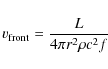
where f is the fraction of mass converted into energy by H burning and other symbols have their usual meaning. Above the front, this velocity is approximately that of matter crossing a given radius to replace H burned below. This velocity is then more properly an inward velocity of matter. The upward drift velocity reduces the flux of say Cr carried inward by matter coming from the surface convection zone, going though the H burning shell and then joining the core.
The Rosseland opacity, as modified by conduction, is shown in the lower left panel of Fig. 5. Slightly below the H burning shell, the opacity becomes dominated by conduction and so rapidly decreases. Close to the H burning shell metals contribute significantly to opacity as shown in Fig. 4.
A zoom of the particle transport around the H burning shell is shown in Fig. 6.
The concentrations are shown in the upper panels at the same two time steps as in Fig. 5.
In the model with diffusion, the strong He gradient created by the H burning shell causes He
to move outwards dragging metals along through an extra contribution to the drift velocity of metals![]() . This leads to the spikes of the drift velocities seen in the middle panels (black lines at
. This leads to the spikes of the drift velocities seen in the middle panels (black lines at
![]() ).
This leads in turn to the small drifting bulges seen in the upper
panels. At the same time, the spikes in the drift velocity reduce the
flux of metals, such as Fe, carried inwards through the burning shell
(at velocity
).
This leads in turn to the small drifting bulges seen in the upper
panels. At the same time, the spikes in the drift velocity reduce the
flux of metals, such as Fe, carried inwards through the burning shell
(at velocity
![]() )
leading to a small underabundance of metals below the shell. The metals
furthermore diffuse towards the center by gravitational settling (aided
by thermal diffusion, ...). Consequently the Fe concentration is
smaller in the model with diffusion than in the intermediate model for
the
)
leading to a small underabundance of metals below the shell. The metals
furthermore diffuse towards the center by gravitational settling (aided
by thermal diffusion, ...). Consequently the Fe concentration is
smaller in the model with diffusion than in the intermediate model for
the
![]() interval even if both models had the same diffusive transport for most
of the evolution, from the ZAMS to well past turnoff. In the model with
diffusion, gravitational settling led to an increase in
interval even if both models had the same diffusive transport for most
of the evolution, from the ZAMS to well past turnoff. In the model with
diffusion, gravitational settling led to an increase in
![]() for
for
![]() .
The concentration variations were calculated for all included species.
They are shown only for P, Cr and Fe but all species not involved in
CNO nor He burning have variations of the same order, though varying in
details.
.
The concentration variations were calculated for all included species.
They are shown only for P, Cr and Fe but all species not involved in
CNO nor He burning have variations of the same order, though varying in
details.
One notes that the diffusion velocity of P caused by
![]() (the red lines in the middle row of Fig. 6)
is very different from that of Cr close to the H burning shell.
For Cr and Fe, in front of the frontier of the He core, this velocity
very nearly equals
(the red lines in the middle row of Fig. 6)
is very different from that of Cr close to the H burning shell.
For Cr and Fe, in front of the frontier of the He core, this velocity
very nearly equals
![]() .
However the total drift velocity (the black lines in the middle row of Fig. 6) is opposite but slightly smaller than the velocity of matter feeding the H burning shell, or
.
However the total drift velocity (the black lines in the middle row of Fig. 6) is opposite but slightly smaller than the velocity of matter feeding the H burning shell, or
![]() .
This leads to a slight reduction of the Cr and Fe flux to the core. It
contributes to the differences seen in the upper panels between the
concentration profiles of the various species. Similar effects are seen
for the other atomic species, not shown in these figures.
.
This leads to a slight reduction of the Cr and Fe flux to the core. It
contributes to the differences seen in the upper panels between the
concentration profiles of the various species. Similar effects are seen
for the other atomic species, not shown in these figures.
Later in the evolution, as the star climbs the RGB, its luminosity increases and so
![]() increases since it is proportional to L (see Eq. (1)). Radiative accelerations also increase with L but not gravitational settling. On figures similar to Fig. 6
(not shown) we have verified this to be the case. The overall effect is
a reduction of the effect of diffusion closer to the He flash.
increases since it is proportional to L (see Eq. (1)). Radiative accelerations also increase with L but not gravitational settling. On figures similar to Fig. 6
(not shown) we have verified this to be the case. The overall effect is
a reduction of the effect of diffusion closer to the He flash.
![\begin{figure}
\par\includegraphics[width=9cm,clip]{12328f7.eps}
\end{figure}](/articles/aa/full_html/2010/02/aa12328-09/img66.png)
|
Figure 7:
Panel a) Inverted |
| Open with DEXTER | |
7  gradient inversion, diffusion and

The effects of concentration variations on ![]() as the H burning shell crosses the region of the concentration discontinuity left by the first dredge-up,
are looked at in detail in Figs. 7 and 8. Consider
as the H burning shell crosses the region of the concentration discontinuity left by the first dredge-up,
are looked at in detail in Figs. 7 and 8. Consider
![]() (where
(where ![]() is the reduced mass per nucleus, that is excluding electrons) defined as the difference between the value of
is the reduced mass per nucleus, that is excluding electrons) defined as the difference between the value of ![]() at a given time step from that at the time step immediately after the first dredge-up; it measures the extent of the
at a given time step from that at the time step immediately after the first dredge-up; it measures the extent of the ![]() inversion. In the upper panel of Fig. 7, at the maximum of
inversion. In the upper panel of Fig. 7, at the maximum of ![]() the value of
the value of
![]() in the model without diffusion (dotted red curve) is a factor of 4.1
smaller than in the model with diffusion (solid red curve). Since the
model with diffusion and the model without diffusion are affected in
the same way by 3He burning, this shows that the main cause of
in the model without diffusion (dotted red curve) is a factor of 4.1
smaller than in the model with diffusion (solid red curve). Since the
model with diffusion and the model without diffusion are affected in
the same way by 3He burning, this shows that the main cause of ![]() inversion when diffusion is properly taken into account is atomic diffusion.
inversion when diffusion is properly taken into account is atomic diffusion.
In panel b, are shown the values of ![]() in a model with diffusion calculated assuming complete ionization
(solid lines). The dot-dashed lines were calculated using ionization
from OPAL tables. The dotted lines were also calculated using
ionization from OPAL tables except that H was assumed completely
ionized showing that it is mainly responsible for the difference
between
in a model with diffusion calculated assuming complete ionization
(solid lines). The dot-dashed lines were calculated using ionization
from OPAL tables. The dotted lines were also calculated using
ionization from OPAL tables except that H was assumed completely
ionized showing that it is mainly responsible for the difference
between ![]() calculated assuming complete ionization and ionization from OPAL tables. The large variation of
calculated assuming complete ionization and ionization from OPAL tables. The large variation of ![]() around the 3He burning region shows that one must carefully calculate ionization if one is to use small
around the 3He burning region shows that one must carefully calculate ionization if one is to use small ![]() inversions to calculate instabilities.
inversions to calculate instabilities.
The advancing burning shell on the bottom panel of Fig. 7 can be linked to the advancing ![]() inversion of panel a and the advancing structures of Fe concentration (panel c).
These are not spurious but are explained by the analysis of
Figs. 5 and 6 in Sect. 6.
Fe underabundances precede the burning front (see the continuous dark
grey curve). The effects of atomic diffusion on the concentration of Fe
and other atomic species and so on
inversion of panel a and the advancing structures of Fe concentration (panel c).
These are not spurious but are explained by the analysis of
Figs. 5 and 6 in Sect. 6.
Fe underabundances precede the burning front (see the continuous dark
grey curve). The effects of atomic diffusion on the concentration of Fe
and other atomic species and so on ![]() can be perceived with difficulty on the continuous dark gray line of
panel a because of the limited resolution of the latter. They are
studied in more detail in Fig. 8.
For that study, it is important that, as one may note from the bottom
panel, most of the models represented by lines of similar color, one
with diffusion (solid) and one without (dotted), are at very nearly the
same evolutionary phase.
can be perceived with difficulty on the continuous dark gray line of
panel a because of the limited resolution of the latter. They are
studied in more detail in Fig. 8.
For that study, it is important that, as one may note from the bottom
panel, most of the models represented by lines of similar color, one
with diffusion (solid) and one without (dotted), are at very nearly the
same evolutionary phase.
![\begin{figure}
\par\mbox{\includegraphics[width=8.5cm]{12328f8a.eps}\hspace{1cm}
\includegraphics[width=8.5cm]{12328f8b.eps} }
\vspace{-1.5mm}\end{figure}](/articles/aa/full_html/2010/02/aa12328-09/img70.png)
|
Figure 8:
Upper left panel Interior profile of |
| Open with DEXTER | |
One may use Fig. 8 to analyze the roles of the atomic diffusion of metals and He as well as of 3He burning in causing small ![]() inversions.
The original discontinuity in the
inversions.
The original discontinuity in the ![]() curve was left over by the first dredge-up; it comes from previous
nuclear evolution and diffusion, mainly during main-sequence evolution.
One notes on the left panel b, the break in
curve was left over by the first dredge-up; it comes from previous
nuclear evolution and diffusion, mainly during main-sequence evolution.
One notes on the left panel b, the break in
![]() created by the mixing of the Fe concentration profile originally caused
by diffusion; it is absent on the right panel b, where diffusion is not
taken into account. For H and He the discontinuities in the
concentration profiles come from both diffusion and nuclear reactions
and are so present in both the model with diffusion and that without
diffusion.
created by the mixing of the Fe concentration profile originally caused
by diffusion; it is absent on the right panel b, where diffusion is not
taken into account. For H and He the discontinuities in the
concentration profiles come from both diffusion and nuclear reactions
and are so present in both the model with diffusion and that without
diffusion.
Proportionately, Fe and He concentrations are affected by diffusion by similar factors but since He is some 50![]() more abundant than metals, its variation is the main cause of variations of
more abundant than metals, its variation is the main cause of variations of ![]() .
Hydrogen and He are even more affected than Fe by diffusion, since the settling of the latter is reduced by
.
Hydrogen and He are even more affected than Fe by diffusion, since the settling of the latter is reduced by
![]() (Fe) (see Figs. 5 and 6)
(Fe) (see Figs. 5 and 6)![]() . Left of the vertical line, the variation of
. Left of the vertical line, the variation of ![]() ,
at the age represented by the green line, (-1.3 Myr) is mainly
caused by H burning while right of it, it is caused by both atomic
diffusion and 3He burning.
One notes in panel a that
,
at the age represented by the green line, (-1.3 Myr) is mainly
caused by H burning while right of it, it is caused by both atomic
diffusion and 3He burning.
One notes in panel a that ![]() decreases by a larger factor (or
decreases by a larger factor (or
![]() has a larger maximum) in the model with diffusion and that the changes
occur there earlier than in the model without diffusion. Indeed a
careful comparison of the right and left c and/or e panels shows that
the change of
has a larger maximum) in the model with diffusion and that the changes
occur there earlier than in the model without diffusion. Indeed a
careful comparison of the right and left c and/or e panels shows that
the change of
![]() and
and
![]() are first caused by atomic diffusion since,
in the interval
are first caused by atomic diffusion since,
in the interval
![]() ,
the dotted dark gray lines for H and He (right panels) are horizontal
while the corresponding full lines have respectively a maximum (left
panel e) and a minimum (left panel c) where they cross the vertical
line;
the increase of the H abundance between the bottom of the convection
zone and the vertical line is caused by atomic diffusion. At that age, 3He burning does contribute additional H but only for smaller values of
,
the dotted dark gray lines for H and He (right panels) are horizontal
while the corresponding full lines have respectively a maximum (left
panel e) and a minimum (left panel c) where they cross the vertical
line;
the increase of the H abundance between the bottom of the convection
zone and the vertical line is caused by atomic diffusion. At that age, 3He burning does contribute additional H but only for smaller values of
![]() .
It is only with the blue line that
.
It is only with the blue line that
![]() burning makes any dent on the H and
burning makes any dent on the H and
![]() concentrations beyond
concentrations beyond
![]() .
With the dotted green line the effect of 3He reaches
.
With the dotted green line the effect of 3He reaches
![]() .
Its effect is clearly seen on the right panels c and e. It leads to a maximum of
.
Its effect is clearly seen on the right panels c and e. It leads to a maximum of
![]() at
at
![]() (see the green dotted curve). This implies that the diffusion of metals and He are the first to cause a reduction of
(see the green dotted curve). This implies that the diffusion of metals and He are the first to cause a reduction of ![]() and, later, the nuclear reactions involving 3He add a contribution. In the model with diffusion, the effect is smaller for
and, later, the nuclear reactions involving 3He add a contribution. In the model with diffusion, the effect is smaller for
![]() but larger for H since for He the effects of diffusion and 3He burning partly cancel while they add for H.
but larger for H since for He the effects of diffusion and 3He burning partly cancel while they add for H.
7.1 Concentration gradients vs turbulence
The preceding results were obtained without any adjustable parameters. The instability created by the ![]() inversion can be simulated by turbulent diffusion.
It remains to determine what value of the turbulent diffusion coefficient starts modifying the results obtained above. Do the
inversion can be simulated by turbulent diffusion.
It remains to determine what value of the turbulent diffusion coefficient starts modifying the results obtained above. Do the ![]() suggested for instance by Charbonnel & Zahn (2007a) modify substantially the small concentration gradients of He and of metals caused by diffusion?
suggested for instance by Charbonnel & Zahn (2007a) modify substantially the small concentration gradients of He and of metals caused by diffusion?
In first approximation, one may write the diffusion velocity equation in the form:
![\begin{displaymath}v_D=(D_{ip}+\ensuremath{D_{\ensuremath{{\mbox{\scriptsize T}}...
...remath{{\mbox{\scriptsize rad}}}}} {}_{,i}-g)+... \right]\cdot
\end{displaymath}](/articles/aa/full_html/2010/02/aa12328-09/img82.png)
Within the first brackets on the right is the purely diffusive term which includes a contribution both from atomic diffusion, Dip, and from turbulent diffusion,

to each element's diffusion velocity, which tends to reduce its abundance gradient in a way very similar to the effect of
The concentration gradients of metals and of He (or H) are very small, yet it is only through those gradients that turbulence (
![]() )
has an effect, whereas atomic diffusion also acts through the much larger g and
)
has an effect, whereas atomic diffusion also acts through the much larger g and
![]() driving terms. Consequently,
driving terms. Consequently,
![]() can have an effect only if it is much larger than the atomic diffusion coefficient, Dip. But how much larger? To have a significant effect on the diffusion velocity,
can have an effect only if it is much larger than the atomic diffusion coefficient, Dip. But how much larger? To have a significant effect on the diffusion velocity,
![]() must lead to a contribution similar to the driving terms of atomic diffusion in Eq. (2). Turbulence then has an effect if
must lead to a contribution similar to the driving terms of atomic diffusion in Eq. (2). Turbulence then has an effect if
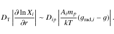
Equation (4) was evaluated roughly using drift velocities of He (similar to those for metals shown on the middle panels of Fig. 5) and the value of
The mixing caused by ![]() gradient inversion is a complex process (see for instance Proffitt 1989) leading to a non-linear diffusion equation since
gradient inversion is a complex process (see for instance Proffitt 1989) leading to a non-linear diffusion equation since
![]() is proportional to the inverted
is proportional to the inverted ![]() gradient. Following Proffitt's formalism, Proffitt & Michaud (1989)
give an approximation to the mixing (their Eqs. (2) to (5))
which is approximately equivalent to the values obtained by Kippenhahn (1974).
However, existing evaluations of
gradient. Following Proffitt's formalism, Proffitt & Michaud (1989)
give an approximation to the mixing (their Eqs. (2) to (5))
which is approximately equivalent to the values obtained by Kippenhahn (1974).
However, existing evaluations of
![]() in the literature, vary by orders of magnitude (see Vauclair 2004; Denissenkov & Pinsonneault 2008; Théado et al. 2009 for recent discussions) mainly because there is no agreement on the size and shape of blobs or fingers.
In their Fig. 2, Charbonnel & Zahn (2007a), using elongated fingers, obtain
in the literature, vary by orders of magnitude (see Vauclair 2004; Denissenkov & Pinsonneault 2008; Théado et al. 2009 for recent discussions) mainly because there is no agreement on the size and shape of blobs or fingers.
In their Fig. 2, Charbonnel & Zahn (2007a), using elongated fingers, obtain
![]() varying from 105 close to the burning shell to 1010 cm2/s
just below the surface convection zone; as mentioned in the last
paragraph of their Sect. 2, this is two orders of magnitude larger
than the estimate of Kippenhahn et al. (1980). They also give corresponding
varying from 105 close to the burning shell to 1010 cm2/s
just below the surface convection zone; as mentioned in the last
paragraph of their Sect. 2, this is two orders of magnitude larger
than the estimate of Kippenhahn et al. (1980). They also give corresponding
![]() as of order 10-5 (see their Fig. 1). We have verified that the
as of order 10-5 (see their Fig. 1). We have verified that the
![]() corresponding to the concentration gradients used to obtain our Fig. 9 are of order 10-4 or some ten times larger. From Eq. (4) reducing the
corresponding to the concentration gradients used to obtain our Fig. 9 are of order 10-4 or some ten times larger. From Eq. (4) reducing the ![]() gradient by a factor of 10 increases
gradient by a factor of 10 increases
![]() by a similar factor or between between 107 and 108 cm2/s. Given that these numbers are within the range of those obtained by
Charbonnel & Zahn (2007a), the settling of 4He could be just as important as 3He burning in creating instabilities between the H burning shell and the surface convection zone.
by a similar factor or between between 107 and 108 cm2/s. Given that these numbers are within the range of those obtained by
Charbonnel & Zahn (2007a), the settling of 4He could be just as important as 3He burning in creating instabilities between the H burning shell and the surface convection zone.
![\begin{figure}
\par\includegraphics[width=8cm]{12328f9.eps} \vspace{-2.5mm} \end{figure}](/articles/aa/full_html/2010/02/aa12328-09/img87.png)
|
Figure 9:
Turbulent diffusion coefficient required to reduce significantly the effect of atomic diffusion as determined from Eq. (4). The color coding is the same as used in the left panels of Fig. 8. Above the burning shell, turbulent diffusion coefficients need to be at least |
| Open with DEXTER | |
8 Conclusion
One would not a priori expect large effects of atomic diffusion in RGB stars. Evolution through that phase is relatively rapid and gravity is small in the atmosphere implying that distances are relatively large so that diffusion is unlikely to have time to modify element concentrations. Surface abundances are not modified by diffusion on the RGB. But while it is true that gravity is small at the surface of RGB stars, it is large around the H burning shell. That is where atomic diffusion ends up playing a role. It was studied most carefully around the luminosity bump (see Sect. 6). In Fig. 6 the drift velocity of metals is shown to be nearly equal to the velocity of the H burning front. Consequently atomic diffusion can modify their concentration. Perhaps the greatest surprise of the results is the relatively important role played by
The effect on the observable properties of RGB stars are however very
small. The most visible effect is at the so called bump region of the
RGB (see the inset in Fig. 1).
The He core mass at the flash of the model with diffusion is slightly
larger than that of the model without diffusion but the difference is
admittedly small: ![]() 0.003
0.003
![]() for the lowest metallicity considered,
Z = 0.0001, to
for the lowest metallicity considered,
Z = 0.0001, to ![]() 0.002
0.002
![]() at solar metallicity.
at solar metallicity.
The ![]() inversion caused by 3He
burning past the luminosity bump was suggested to be the main cause of
mixing between the H burning shell and the surface convection zone
(Eggleton et al. 2008; Charbonnel & Zahn 2007a; Eggleton et al. 2006).
The gravitational settling of He between the surface convection zone
and the H burning shell has been found to lead to a
inversion caused by 3He
burning past the luminosity bump was suggested to be the main cause of
mixing between the H burning shell and the surface convection zone
(Eggleton et al. 2008; Charbonnel & Zahn 2007a; Eggleton et al. 2006).
The gravitational settling of He between the surface convection zone
and the H burning shell has been found to lead to a ![]() gradient inversion larger by a factor of
gradient inversion larger by a factor of
![]() than the
than the ![]() inversion 3He burning leads to (see Sect. 7). It has also been shown to occur slightly earlier during evolution. However the inversion created by 3He burning is replenished on 3He burning time scale whereas the settling of H is determined by the atomic diffusion time scale.
inversion 3He burning leads to (see Sect. 7). It has also been shown to occur slightly earlier during evolution. However the inversion created by 3He burning is replenished on 3He burning time scale whereas the settling of H is determined by the atomic diffusion time scale.
The results presented in this paper were obtained entirely from first principles. We do not wish to imply that there is no
role for turbulence either from differential rotation or related to the appearance of inverse ![]() gradients. However
the comparison of the turbulent diffusion coefficients required to wipe out the effects of diffusion on the RGB (see Sect. 7.1)
puts limits on the values of turbulent transport and on its causes.
Atomic diffusion could be the main cause of the instability generated
by an inverted
gradients. However
the comparison of the turbulent diffusion coefficients required to wipe out the effects of diffusion on the RGB (see Sect. 7.1)
puts limits on the values of turbulent transport and on its causes.
Atomic diffusion could be the main cause of the instability generated
by an inverted ![]() gradient.
gradient.
As mentioned at the end of Sect. 6, settling becomes less important as the star approaches the He flash. Consequently the mixing He settling can lead to is also progressively reduced past the luminosity bump. This appears consistent with the observational result that mixing on the RGB seems to occur mainly immediately past the bump (see the Introduction of Denissenkov & VandenBerg 2003).
AcknowledgementsThis research was partially supported at the Université de Montréal by NSERC. We thank the Réseau québécois de calcul de haute performance (RQCHP) for providing us with the computational resources required for this work. We thank Don VandenBerg for useful discussions and a careful reading of the manuscript and Santi Cassisi for his constructive review of the paper.
References
- Cassisi, S., degl'Innocenti, S., & Salaris, M. 1997, MNRAS, 290, 515 [NASA ADS] [CrossRef] [Google Scholar]
- Cassisi, S., Castellani, V., degl'Innocenti, S., et al. 1998, A&AS, 129, 267 [Google Scholar]
- Charbonnel, C., & Zahn, J.-P. 2007a, A&A, 467, L15 [NASA ADS] [CrossRef] [EDP Sciences] [Google Scholar]
- Charbonnel, C., & Zahn, J.-P. 2007b, A&A, 476, L29 [NASA ADS] [CrossRef] [EDP Sciences] [Google Scholar]
- Denissenkov, P. A., & Pinsonneault, M. 2008, ApJ, 684, 626 [NASA ADS] [CrossRef] [Google Scholar]
- Denissenkov, P. A., & VandenBerg, D. A. 2003, ApJ, 593, 509 [NASA ADS] [CrossRef] [Google Scholar]
- Eggleton, P. P. 1971, MNRAS, 151, 351 [NASA ADS] [CrossRef] [Google Scholar]
- Eggleton, P. P., Dearborn, D. S. P., & Lattanzio, J. C. 2006, Sci, 314, 1580 [Google Scholar]
- Eggleton, P. P., Dearborn, D. S. P., & Lattanzio, J. C. 2008, ApJ, 677, 581 [NASA ADS] [CrossRef] [Google Scholar]
- Kippenhahn, R. 1974, in Late Stages of Stellar Evolution, ed. R. J. Tayler, & J. E. Hesser, 20 [Google Scholar]
- Kippenhahn, R., Ruschenplatt, G., & Thomas, H.-C. 1980, A&A, 91, 175 [NASA ADS] [Google Scholar]
- Michaud, G., Richer, J., & Richard, O. 2007, ApJ, 670, 1178 [NASA ADS] [CrossRef] [Google Scholar]
- Michaud, G., Richer, J., & Richard, O. 2008, ApJ, 675, 1223 [NASA ADS] [CrossRef] [Google Scholar]
- Proffitt, C. R. 1989, ApJ, 338, 990 [NASA ADS] [CrossRef] [Google Scholar]
- Proffitt, C. R., & Michaud, G. 1989, ApJ, 345, 998 [NASA ADS] [CrossRef] [Google Scholar]
- Proffitt, C. R., & VandenBerg, D. A. 1991, ApJS, 77, 473 [NASA ADS] [CrossRef] [Google Scholar]
- Richard, O., Michaud, G., & Richer, J. 2001, ApJ, 558, 377 [NASA ADS] [CrossRef] [Google Scholar]
- Richard, O., Michaud, G., Richer, J., et al. 2002, ApJ, 568, 979 [Google Scholar]
- Richer, J., Michaud, G., Rogers, F., et al. 1998, ApJ, 492, 833 [NASA ADS] [CrossRef] [Google Scholar]
- Rogers, F. J., & Iglesias, C. A. 1992a, ApJS, 79, 507 [NASA ADS] [CrossRef] [Google Scholar]
- Rogers, F. J., & Iglesias, C. A. 1992b, ApJ, 401, 361 [NASA ADS] [CrossRef] [Google Scholar]
- Rogers, F. J., Swenson, F. J., & Iglesias, C. A. 1996, ApJ, 456, 902 [NASA ADS] [CrossRef] [Google Scholar]
- Sweigart, A. V., & Gross, P. G. 1978, ApJS, 36, 405 [NASA ADS] [CrossRef] [Google Scholar]
- Sweigart, A. V., & Mengel, J. G. 1979, ApJ, 229, 624 [NASA ADS] [CrossRef] [Google Scholar]
- Théado, S., Vauclair, S., Alecian, G., et al. 2009, ApJ, 704, 1262 [NASA ADS] [CrossRef] [Google Scholar]
- Turcotte, S., Richer, J., Michaud, G., Iglesias, C., & Rogers, F. 1998, ApJ, 504, 539 [NASA ADS] [CrossRef] [Google Scholar]
- Ulrich, R. K. 1972, ApJ, 172, 165 [NASA ADS] [CrossRef] [Google Scholar]
- VandenBerg, D. A. 1992, ApJ, 391, 685 [NASA ADS] [CrossRef] [Google Scholar]
- VandenBerg, D. A., Swenson, F. J., Rogers, F. J., Iglesias, C. A., & Alexander, D. R. 2000, ApJ, 532, 430 [NASA ADS] [CrossRef] [Google Scholar]
- Vauclair, S. 2004, ApJ, 605, 874 [NASA ADS] [CrossRef] [Google Scholar]
- Zahn, J.-P. 1992, A&A, 265, 115 [NASA ADS] [Google Scholar]
Footnotes
- ... metallicities
![[*]](/icons/foot_motif.png)
- In this series of papers, the relative values of the
 elements are increased following VandenBerg
et al. (2000). Models are labeled according to their
original Z value calculated before the
correction. See also Table 1 of Richard et al. (2002).
This correction was not applied in the Z = 0.02
models.
elements are increased following VandenBerg
et al. (2000). Models are labeled according to their
original Z value calculated before the
correction. See also Table 1 of Richard et al. (2002).
This correction was not applied in the Z = 0.02
models.
- ... diffusion
- For instance, inspired by the method developed by Eggleton (1971), VandenBerg (1992) prefers to switch, as described in his Sect. 3, to a non-Lagrangian mesh for his RGB calculations.
- ... diffusion
- The model with semi-convection has a core mass
 larger and the model without
  ,
a core mass
smaller than the model with diffusion.
,
a core mass
smaller than the model with diffusion.
- ... there
- See the end of Sect. 2 of Cassisi et al. (1997).
- ... diffusion
- This is based on as yet unpublished calculations.
- ... panel
- The function ``linlog'' used in some of the figures is
defined by
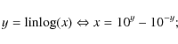
it is a kind of base 10 arcsinh function, useful for displaying both large and small, positive and negative values of the same function. For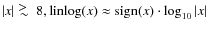 ,
and for
,
and for  ,
,
 .
.
- ... state
- In addition to the spectra they used to construct opacities, OPAL included the mean charge of each atomic species on its grid. See Richer et al. (1998); Rogers & Iglesias (1992a,b); Rogers et al. (1996).
- ... metals
- The effect of a steep He gradient of the drift velocity of metals is described in slightly more detail in the second paragraph of Sect. 3.1.3. of Richard et al. (2001).
- ...)
- This is an example where the inclusion of the gravitational
settling of metals improves the accuracy of the calculations only
if
are also included.
All Figures
|
|
Figure 1:
Left panel: HR diagram for
four models with Z = 0.004;
red: with diffusion, green: with diffusion and semi-convection during
dredge-up, gray: model without diffusion, blue: intermediate model. The
intermediate model parted from the models with diffusion past turnoff
at the point indicated by |
| Open with DEXTER | |
| In the text | |
|
|
Figure 2:
Size of He core as a function of 3 |
| Open with DEXTER | |
| In the text | |
|
|
Figure 3:
Internal properties of three RG models at approximately the same He luminosity during the He flash. On panel a)
is seen the convection zone generated by the flash for the model with
diffusion (red lines), the model without diffusion (solid gray line)
and the intermediate model (dot-dashed blue line). As the flash begins,
the interior limit of the convection is at very nearly the same mass.
On panels b) and c) are shown respectively the Fe and 12C abundances. On the bottom panel, e),
is shown the He nuclear energy generation for the model with diffusion
for two different time steps (red lines) which bracket the energy
generation of the model without diffusion and of the intermediate
model. The dotted line is for the neutrino energy. On panel d),
one sees that outside the flash area, the opacity (here corrected for
conduction; the dotted black line represents conduction only) is nearly
the same in all models. In the zoomed inset, one may see that the
opacities of the model with diffusion (solid and dashed lines) and of
the intermediate model (dot-dashed blue line) are some 4% smaller than
that of the model without diffusion (solid gray line). Especially for
|
| Open with DEXTER | |
| In the text | |
|
|
Figure 4: Ratio of the Rosseland
opacity (here including the effect of conduction) evaluated without
including the spectrum of the element of atomic number Z
and of that obtained with the complete mix (24 elements). The
concentration of each remaining species is increased to maintain
normalization. It is shown at
|
| Open with DEXTER | |
| In the text | |
|
|
Figure 5:
Mass fractions ( upper panels)
and drift velocities (central panels) of P (left panels), Cr (central
panels) and Fe (right panels) as a function of the mass interior
to r, shortly after the maximum inward extension of the
surface convection zone: more precisely when the H burning shell
crosses the concentration jump left by the convection zone. Two ages
are shown for the model with diffusion at -7.7 Myr (dashed brown
line) and -2.9 Myr (solid red line) with respect to
|
| Open with DEXTER | |
| In the text | |
|
|
Figure 6:
The upper panels are a zoom around the H burning shell of mass fractions of P, Cr and Fe shown in Fig. 5 at the same ages as on that figure where the curves are identified. The middle panels give (with
v0 = 10-9 cm/s) the total drift
velocity (black lines), the radiative acceleration contribution to the
drift velocity (brown dashed line and red solid line) and the front
velocity (see Eq. (1);
blue lines) which is approximately that of matter crossing a given
radius to replace H burned below. All three velocities are of the
same order. Radiative accelerations of Fe, Cr and P are shown on
the lower panels where dotted lines represent gravity. The
radiative accelerations are larger than gravity above the
H burning shell for the three elements. The
|
| Open with DEXTER | |
| In the text | |
|
|
Figure 7:
Panel a) Inverted |
| Open with DEXTER | |
| In the text | |
|
|
Figure 8:
Upper left panel Interior profile of |
| Open with DEXTER | |
| In the text | |
|
|
Figure 9:
Turbulent diffusion coefficient required to reduce significantly the effect of atomic diffusion as determined from Eq. (4). The color coding is the same as used in the left panels of Fig. 8. Above the burning shell, turbulent diffusion coefficients need to be at least |
| Open with DEXTER | |
| In the text | |
Copyright ESO 2010
Current usage metrics show cumulative count of Article Views (full-text article views including HTML views, PDF and ePub downloads, according to the available data) and Abstracts Views on Vision4Press platform.
Data correspond to usage on the plateform after 2015. The current usage metrics is available 48-96 hours after online publication and is updated daily on week days.
Initial download of the metrics may take a while.