| Issue |
A&A
Volume 510, February 2010
|
|
|---|---|---|
| Article Number | A94 | |
| Number of page(s) | 5 | |
| Section | Planets and planetary systems | |
| DOI | https://doi.org/10.1051/0004-6361/200912052 | |
| Published online | 17 February 2010 | |
Transit timing analysis of CoRoT-1b![[*]](/icons/foot_motif.png) (Research Note)
(Research Note)
Sz. Csizmadia1 - S. Renner2,3 - P. Barge4 - E. Agol5 - S. Aigrain6 - R. Alonso4,7 - J.-M. Almenara8 - A. S. Bonomo4,9 - P. Bordé10 - F. Bouchy11 - J. Cabrera1,12 - H. J. Deeg8 - R. De la Reza13 - M. Deleuil4 - R. Dvorak14 - A. Erikson1 - E. W. Guenther8,15 - M. Fridlund16 - P. Gondoin11 - T. Guillot17 - A. Hatzes15 - L. Jorda4 - H. Lammer18 - C. Lázaro11,19 - A. Léger10 - A. Llebaria4 - P. Magain20 - C. Moutou4 - M. Ollivier10 - M. Pätzold21 - D. Queloz7 - H. Rauer1,22 - D. Rouan23 - J. Schneider12 - G. Wuchterl15 - D. Gandolfi15
1 - Institute of Planetary Research, DLR, Rutherfordstr. 2,
12489 Berlin, Germany
2 -
Institut de Mécanique Céleste et de Calcul de Éphémérides,
UMR 8028 du CNRS, 77 avenue Denfert-Rochereau, 75014 Paris, France
3 -
Laboratoire d'Astronomie de Lille,
Université Lille 1, 1 impasse de l'observatoire, 59000 Lille, France
4 -
Laboratoire d'Astrophysique de Marseille,
UMR 6110, CNRS/Université de Provence, 38 rue F. Joliot-Curie, 13388
Marseille, France
5 -
Department of Astronomy, University of Washington, Box 351580, Seattle,
WA 98195, USA
6 -
School of Physics, University of Exeter, Stocker Road, Exeter EX4
4QL, UK
7 -
Observatoire de Genève, Université de Genève, 51 chemin des
Maillettes, 1290 Sauverny, Switzerland
8 -
Instituto de Astrofísica de Canarias, 38205 La Laguna, Tenerife,
Spain
9 -
INAF - Osservatorio Astrofisico di Catania, via S. Sofia 78,
95123 Catania, Italy
10 -
Institut d'Astrophysique Spatiale, Université Paris XI, 91405
Orsay, France
11 -
Institut d'Astrophysique de Paris, Université Pierre & Marie
Curie, 98bis Bd Arago, 75014 Paris, France
12 -
LUTH, Observatoire de Paris, CNRS, Université Paris Diderot, 5
place Jules Janssen, 92190 Meudon, France
13 -
Observatório Nacional, Rio de Janeiro, RJ, Brazil
14 -
University of Vienna, Institute of Astronomy, Türkenschanzstr. 17,
1180 Vienna, Austria
15 -
Thüringer Landessternwarte, Sternwarte 5, Tautenburg 5, 07778
Tautenburg, Germany
16 -
Research and Scientific Support Department, ESTEC/ESA, PO Box 299,
2200 AG Noordwijk, The Netherlands
17 -
Observatoire de la Côte d'Azur, Laboratoire Cassiopée, BP 4229,
06304 Nice Cedex 4, France
18 -
Space Research Institute, Austrian Academy of Science,
Schmiedlstr. 6, 8042 Graz, Austria
19 -
Departamento de Astrofísica, Universidad de La Laguna, 38205 La
Laguna, Tenerife, Spain
20 -
University of Liège, Allée du 6 août 17, Sart Tilman, Liège
1, Belgium
21 -
Rheinisches Institut für Umweltforschung an der Universität zu
Köln, Aachener Strasse 209, 50931 Köln, Germany
22 -
Center for Astronomy and Astrophysics, TU Berlin,
Hardenbergstr. 36, 10623 Berlin, Germany
23 -
LESIA, UMR 8109 CNRS, Observatoire de Paris, UVSQ, Université
Paris-Diderot, 5 place J. Janssen, 92195 Meudon, France
Received 12 March 2009 / Accepted 26 October 2009
Abstract
Context. CoRoT, the pioneer space-based transit search,
steadily provides thousands of high-precision light curves with
continuous time sampling over periods of up to 5 months. The
transits of a planet perturbed by an additional object are not strictly
periodic. By studying the transit timing variations (TTVs), additional
objects can be detected in the system.
Aims. A transit timing analysis of CoRoT-1b is carried out to constrain the existence of additional planets in the system.
Methods. We used data obtained by an improved version of the
CoRoT data pipeline (version 2.0). Individual transits were fitted to
determine the mid-transit times, and we analyzed the derived O-C
diagram. N-body integrations were used to place limits on secondary planets.
Results. No periodic timing variations with a period shorter
than the observational window (55 days) are found. The presence of
an Earth-mass Trojan is not likely. A planet of mass greater than ![]() 1
Earth mass can be ruled out by the present data if the object is in a
2:1 (exterior) mean motion resonance with CoRoT-1b. Considering
initially circular orbits: (i) super-Earths (less than 10 Earth-masses)
are excluded for periods less than about 3.5 days; (ii)
Saturn-like planets can be ruled out for periods less than about
5 days; (iii) Jupiter-like planets should have a minimum orbital
period of about 6.5 days.
1
Earth mass can be ruled out by the present data if the object is in a
2:1 (exterior) mean motion resonance with CoRoT-1b. Considering
initially circular orbits: (i) super-Earths (less than 10 Earth-masses)
are excluded for periods less than about 3.5 days; (ii)
Saturn-like planets can be ruled out for periods less than about
5 days; (iii) Jupiter-like planets should have a minimum orbital
period of about 6.5 days.
Key words: planetary systems - techniques: photometric - methods: numerical - occultations
1 Introduction
As a consequence of the gravitational perturbations, the mid-times of consecutive transits deviate from a linear ephemeris in a transiting exoplanet system (transit timing variation, hereafter TTV). Depending on the mass and the orbital configuration of the perturbing planet, this deviation can have amplitudes from a few seconds to days (e.g. Steffen 2006). Moreover, the duration, shape, and depth of the transits can also change. In extreme cases the transits can disappear and then reappear (Schneider 1994, 2004). Both the theoretical aspects and the observable effects have been studied in e.g. Miralda-Escudé (2002), Borkovits et al. (2003), Agol et al. (2005), Holman & Murray (2005), Ford & Holman (2007), Simon et al. (2007), Heyl & Gladman (2007), Nesvorný & Morbidelli (2008), Pál & Kocsis (2008) and Kipping (2009). Several transiting exoplanets were subject to this kind of analysis (Steffen & Agol 2005; Agol & Steffen 2007; Miller-Ricci et al. 2007; Alonso et al. 2009; Hrudková et al. 2008; Miller-Ricci et al. 2008a,b; Diaz et al. 2008; Coughlin et al. 2008; Rabus et al. 2009; Stringfellow et al. 2009).
| Figure 1: Top: a typical transit observation of CoRoT-1b by CoRoT in the 512 s sampling rate mode. Bottom: a typical transit observation of CoRoT-1b by CoRoT in the 32 s sampling rate mode. Abcissa is phase, ordinate is normalized intensity. The solid lines show the fit. |
|
| Open with DEXTER | |
In addition, stellar spots may affect the transit shape and, because of this, we have some difficulty in determining of the midtime of the transit. This effect may cause spurious periodic terms in the O-C diagram of exoplanets (Alonso et al. 2009; Pont et al. 2007).
Here we report the TTV analysis of CoRoT-1b based on data obtained by an
improved version of the CoRoT data pipeline. In this system a low-density
planet (mass: 1.03
![]() ,
radius: 1.49
,
radius: 1.49
![]() ,
average density:
0.38 g cm-3, semi-major axis: 5.46
,
average density:
0.38 g cm-3, semi-major axis: 5.46 ![]() ,
orbital period: 1.5089557 days) orbits a G2 main-sequence star (Barge et al. 2008). Thirty-six transits
were observed by CoRoT, 20 of them in 512 s and 16 with the 32 s
sampling rate mode. In total more than 68 000 data points were collected during
55 consecutive days (Barge et al. 2008). The operation of the satellite is
described in detail in the pre-launch book, and the reader can find useful
information about CoRoT in Baglin et al. (2007), Boisnard et al. (2006), and
Auvergne et al. (2009).
,
orbital period: 1.5089557 days) orbits a G2 main-sequence star (Barge et al. 2008). Thirty-six transits
were observed by CoRoT, 20 of them in 512 s and 16 with the 32 s
sampling rate mode. In total more than 68 000 data points were collected during
55 consecutive days (Barge et al. 2008). The operation of the satellite is
described in detail in the pre-launch book, and the reader can find useful
information about CoRoT in Baglin et al. (2007), Boisnard et al. (2006), and
Auvergne et al. (2009).
2 Methods of mid-transit point determination: effect of the sampling rate on the precision
If one uses the CoRoT data for TTV analysis, the main limiting factor
arises from the sampling rate. The typical length of the ingress/egress
phase of a hot Jupiter is on the order of 10-20 min (in the
particular case of CoRoT-1b, the ingress/egress time is 9.8 min)
CoRoT targets are observed with 512 or 32 s sampling rates (the
so-called undersampled/oversampled modes, see Fig. 1). Concerning a
typical 3 h transit, one can easily conclude that a transit
observation consists of only
![]() data
points. In the oversampled mode
we have typically over 300 data points per transit. The small
number of
data points in the undersampled mode may not be balanced by the very
good photometric precision of CoRoT (which is about 0.1% for a
13 mag star in white light for a 512 s exposure, see Auvergne
et al. 2009), therefore we chose to investigate this issue.
data
points. In the oversampled mode
we have typically over 300 data points per transit. The small
number of
data points in the undersampled mode may not be balanced by the very
good photometric precision of CoRoT (which is about 0.1% for a
13 mag star in white light for a 512 s exposure, see Auvergne
et al. 2009), therefore we chose to investigate this issue.
A second factor arises from the orbit of the satellite. The satellite periodically crosses the so-called South Atlantic Anomaly (SAA) region, which causes bad/uncertain data points and long data gaps (typically 10 min). This is significant only when the SAA-crossing occurs during the ingress or the egress phase. Therefore the following test was carried out. Using the exoplanet light curve model of Mandel & Agol (2002) and the parameters of the system (Barge et al. 2008), we simulated the light curve of CoRoT-1b. Then this curve was re-sampled to the same time-points as CoRoT observations. We added a Gaussian-like random noise to the points. The standard deviation of the noise term was chosen in such a way that we had the same signal-to-noise ratio as given in Barge et al. (2008) for the CoRoT-1 light curve. A constant orbital period was assumed.
![\begin{figure}
\par\includegraphics[width=7.2cm,clip]{12052_fig3.eps}\hspace*{8mm}
\includegraphics[width=6.6cm,clip]{12052_fig4.eps}
\end{figure}](/articles/aa/full_html/2010/02/aa12052-09/img7.png)
|
Figure 2: Top: the O-C diagram of CoRoT-1b obtained by the light curve fit of the individual transits. Bottom: the power spectrum of the Fourier-transform of the O-C diagram. Frequency is in cycles/day and amplitude is in seconds. |
| Open with DEXTER | |
Then we determined the mid-transit times in this simulated light curve,
fitting each individual transit separately. Again, we use the
Mandel & Agol (2002) model combined with the Amoeba algorithm (Press et al. 1992) to find the optimum fit. We assumed that the planet-to-stellar
radius ratio and the limb-darkening coefficients are known, so they were fixed.
The adjustable parameters are the mid-transit point, the inclination, and the
![]() ratio (a: semi-major axis,
ratio (a: semi-major axis, ![]() :
stellar radius).
:
stellar radius).
On average, the fits of the individual transits yield only a difference of 9 s between the real and the determined midtransit points in the undersampled mode, when there are data points in the ingress/egress part of the light curve. When the ingress or egress part is missing in the undersampled mode, the errors can be as large as 20-60 s, depending on the distribution of points during the transit. If both the ingress and egress parts are missing, the errors are 60-120 s, sometimes even more.
These optimistic error bars should be increased due to at least two different effects. First, we do not know a priori the exact value of the orbital period which leads to small uncertainties in the calculation of the phase. We estimate that for CoRoT-1b this is negligible. Second, the stellar activity is not included. However, the detailed discussion of these two effects goes beyond the purpose of the present investigation.
Since we use a constant period and assume e=0 during the simulation, we
expect a linear O-C curve with some scatter. To better
characterize this scatter we calculate the standard deviation of the
sample. We find that the mean ![]() scatter of the resulting overall
O-C diagram of this simulated light curve with a constant period
is 22 s. But it is 27 s for the undersampled part and
16 s
for the oversampled part.
scatter of the resulting overall
O-C diagram of this simulated light curve with a constant period
is 22 s. But it is 27 s for the undersampled part and
16 s
for the oversampled part.
3 TTV analysis of CoRoT-1b
We used the N2 level data points (Auvergne et al. 2009) processed by the 2.0 version of the pipeline (not yet realeased data for the public). The resulting light curve was manually checked: a few data points were noted by the pipeline to be affected by cosmic ray events in spite of it having no problems - we restored these data points. In addition, several outliers were removed by hand. Then we performed a TTV analysis by fitting all transits using the method described in the previous section. Transit No. 30 is excluded from this investigation because it is strongly affected by noise. Table 1 gives the midtransit times and their errors.
Table 1: Mid-transit times (HJD) and errors (days) of CoRoT-1b.
The overall O-C diagram and its Fourier-transform are given in Fig. 2.
This diagram is built using the observed light curve. It is prominent
that after switching on the 32 s sampling rate mode (after the 20th transit),
the ![]() scatter of the O-C diagram is reduced to only 18 s, compared to
the
scatter of the O-C diagram is reduced to only 18 s, compared to
the ![]() scatter of the 25 s observed in the undersampled mode. The
scatter of the 25 s observed in the undersampled mode. The
![]() scatter of the whole O-C diagram is 22 s. All these scatter
values are very close to the value we would expect in the case of a constant
orbital period (see previous section).
scatter of the whole O-C diagram is 22 s. All these scatter
values are very close to the value we would expect in the case of a constant
orbital period (see previous section).
Table 2: Amplitudes and periods of O-C variations in CoRoT-1b system.
No clear periodicity or trend can be identified in this diagram. We calculate
the Fourier-spectrum of the O-C curve by the Period04 software (Lenz & Breger 2005) to
search for any non-obvious periodicity. The power spectrum shows few peaks,
but none of them is above the noise level. The highest peak has only
![]() ,
so it is not regarded as a real signal.
,
so it is not regarded as a real signal.
We conclude that there are not any periodic TTVs in CoRoT-1b with a period
less than the observational window (55 days) and an amplitude larger than
about 1 min (=![]() detection level). We also note that there is no
significant change in the inclination and the
detection level). We also note that there is no
significant change in the inclination and the
![]() ratio during this
interval. Bean (2009) presents results about the TTV analysis of CoRoT-1b
based on the public data processed by an earlier version of the
pipeline. His O-C diagram shows a larger
ratio during this
interval. Bean (2009) presents results about the TTV analysis of CoRoT-1b
based on the public data processed by an earlier version of the
pipeline. His O-C diagram shows a larger ![]() -scatter (36 s
compared to our 22 s).
-scatter (36 s
compared to our 22 s).
4 Limits on secondary planets
4.1 Examples of simulated TTVs
We show in Table 2 which amplitudes and periods can typically be
expected in the O-C diagram of the CoRoT-1b system based on some
dynamical simulations. We include an Earth-mass planet at the L4Lagrangian point, an Earth in the 2:1 exterior mean motion resonance, a
nearby Neptune-like planet, or an outer eccentric Neptune. The stellar
mass, the mass of CoRoT-1b and its orbital elements are fixed to the
values given in Barge et al. (2008). We use the Mercury software
(Chambers 1999), with the Burlish-Stoer algorithm (accuracy parameter
![]() ). As one can see in Table 2, O-C variations on the
order of 60-150 s might occur on a short time scale (typically
10-150 orbital cycles of the transiting planet).
). As one can see in Table 2, O-C variations on the
order of 60-150 s might occur on a short time scale (typically
10-150 orbital cycles of the transiting planet).
Case 1: an Earth-mass Trojan planet librating with an amplitude of ![]() around
the L4 Lagrangian point would have an amplitude of 60 s in the O-C diagram with a
period of about 10 orbital cycles of the transiting planet (about 15 days, see Table 2).
The amplitude is close to our detection limit. There is a peak in
the Fourier-spectrum of the O-C diagram at the corresponding frequency with an amplitude
of about 11 s. However, the peak is not significant (
around
the L4 Lagrangian point would have an amplitude of 60 s in the O-C diagram with a
period of about 10 orbital cycles of the transiting planet (about 15 days, see Table 2).
The amplitude is close to our detection limit. There is a peak in
the Fourier-spectrum of the O-C diagram at the corresponding frequency with an amplitude
of about 11 s. However, the peak is not significant (
![]() only). Therefore,
an additional planet with similar parameters is not likely.
only). Therefore,
an additional planet with similar parameters is not likely.
![\begin{figure}
\includegraphics[width=8cm,clip]{12052_fig5.ps}
\end{figure}](/articles/aa/full_html/2010/02/aa12052-09/img17.png)
|
Figure 3: The simulated O-C diagram of CoRoT-1b if the transiting planet is perturbed by an Earth-mass planet initially on a circular orbit in 2:1 mean motion resonance. |
| Open with DEXTER | |
Case 2: an Earth-mass planet initially on a circular orbit and in 2:1 mean motion resonance with CoRoT-1b would have an amplitude of about 100 s in the O-C diagram with a period of about 150 transits (approximately 225 days, see Table 2 and Fig. 3). If the CoRoT observational window was around the maximum or the minimum of the O-C curve (see Fig. 3) then we would have no chance to discover this possible planet because the amplitude is on the order of the scatter. If the observational window matched the steepest part of the O-C diagram, we would observe a linear O-C curve that could be interpreted as a wrong period value. This gives a hint: if there are no observed period variations in a short observational window, this does not mean that we can give an upper limit for a hypothetical perturber object. It might be the case that we are on a linear part of the O-C curve. The observational window should be long enough to exclude similar cases.
Cases 3 and 4: simulations show that an outer 30 Earth-mass planet, close to CoRoT-1b ( P=2.772118632 days and e=0.05) or eccentric ( P=4.2679123 days and e=0.25), cause O-C variations of about 150 s, within approximately 15 and 30 orbital revolutions of the transiting planet, respectively (see Table 2). This is much greater than our detection limit, so outer planets in the CoRoT-1b system with similar orbital parameters can be excluded.
4.2 Detailed analysis
Using N-body integrations, we computed the maximum mass of a hypothetical
perturbing planet, with given initial orbital periods and eccentricities,
leading to TTVs compatible with the data. To calculate the transit times, we
used a bracketing routine from Agol et al. (2005). The orbits of CoRoT-1b and an
additional planet were computed over the timespan of the observations, using a
Burlish-Stoer integrator with an accuracy parameter
![]() .
The
equations of motion were integrated in a Cartesian reference frame centered on
the barycenter of the system. The transit times are subtracted from the data to
give the O-C residuals and
.
The
equations of motion were integrated in a Cartesian reference frame centered on
the barycenter of the system. The transit times are subtracted from the data to
give the O-C residuals and ![]() .
.
![\begin{figure}
\includegraphics[width=8cm,clip]{12052_fig6.ps}
\end{figure}](/articles/aa/full_html/2010/02/aa12052-09/img19.png)
|
Figure 4: Maximum allowed mass of a hypothetical perturbing object as a function of its orbital period for excentricities e=0 and 0.2. The 2:1 mean motion resonance is indicated. |
| Open with DEXTER | |
The masses of the central star and
CoRoT-1b are respectively fixed at 0.95 solar masses and 1.03 Jupiter masses
(Barge et al. 2008). The orbit of CoRoT-1b is initially circular with an orbital
period
P=1.5089557 d (Barge et al. 2008) and a true longitude
![]() deg. With these parameters and without any perturbation due to an additional body,
the first transit occurs at
T(HJD)=2454138.327840, and the residuals given by
the numerical integration are at their minimum (i.e. the same as the ones from the best constant
period fit, see Sect. 3) with the following values: zero mean, standard deviation
deg. With these parameters and without any perturbation due to an additional body,
the first transit occurs at
T(HJD)=2454138.327840, and the residuals given by
the numerical integration are at their minimum (i.e. the same as the ones from the best constant
period fit, see Sect. 3) with the following values: zero mean, standard deviation
![]() s,
s,
![]() .
.
The perturbing planet is assumed to be in the same plane as CoRoT-1b.
For given initial orbital parameters, we increase the mass of the test
planet, starting at 0.1 Earth masses, and calculate the standard
deviation of the O-C residuals. We store the mass value for which this
rms exceeds the observed scatter
![]() .
In this way we
determine the maximum planet's mass allowed. The results are shown in
Fig. 4 (respectively Fig. 5), which shows the maximum mass for a
perturbing object as a function of its initial orbital period (resp.
initial orbital period and eccentricity). In Fig. 4, the mass of the
secondary planet has been varied between 0.1 and 100 Earth masses (100
values on a log scale), and its initial orbital period between 2.8 and
7.6 days (with a step of 0.0015 days). For any given orbital
period, eccentricity, and mass value, the TTV-signal is computed over
the range of possible initial true anomaly and longitude of pericenter
values to minimize the resulting residuals. In Fig. 5,
the perturbing
planet is initially at its apocenter (fixed at 180 degrees from
CoRoT-1b), and the following grid of parameters has been used: (i)
masses between 0.1 and 100 Earth masses (100 values on a log
scale);
(ii) orbital periods between 2.8 and 7.6 days (with a step of
0.001333 days); (iii) eccentricities between 0 and 0.25 (100
values on a log
scale).
.
In this way we
determine the maximum planet's mass allowed. The results are shown in
Fig. 4 (respectively Fig. 5), which shows the maximum mass for a
perturbing object as a function of its initial orbital period (resp.
initial orbital period and eccentricity). In Fig. 4, the mass of the
secondary planet has been varied between 0.1 and 100 Earth masses (100
values on a log scale), and its initial orbital period between 2.8 and
7.6 days (with a step of 0.0015 days). For any given orbital
period, eccentricity, and mass value, the TTV-signal is computed over
the range of possible initial true anomaly and longitude of pericenter
values to minimize the resulting residuals. In Fig. 5,
the perturbing
planet is initially at its apocenter (fixed at 180 degrees from
CoRoT-1b), and the following grid of parameters has been used: (i)
masses between 0.1 and 100 Earth masses (100 values on a log
scale);
(ii) orbital periods between 2.8 and 7.6 days (with a step of
0.001333 days); (iii) eccentricities between 0 and 0.25 (100
values on a log
scale).
From Fig. 4, Saturn-like planets can be ruled out for periods less
than about 5 days if e=0 (respectively 6 days if e=0.2). As shown in the
figures, perturbing planets with eccentric orbits obviously cause larger
TTVs, hence have lower mass limits. Super-Earths are defined as
planets with 1-10 Earth masses (Valencia et al. 2007). Depending on the
initial eccentricity, such planets with orbital periods less than
3.4-4.1 days can be excluded. Planets with masses greater than 0.3-1.0
Earth masses can be ruled out by the data if they are in the 2:1
(exterior) mean motion resonance with CoRoT-1b. The data do
not allow strongly constraining the mass of perturbing planets near
higher order resonances. Finally, we estimate the minimum orbital
period for an outer Jupiter-mass planet. From Holman & Murray (2005),
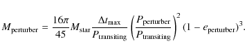
|
(1) |
When assuming a circular orbit and
![\begin{figure}
\includegraphics[angle=270,width=9cm,clip]{12052_fig7.ps}
\end{figure}](/articles/aa/full_html/2010/02/aa12052-09/img26.png)
|
Figure 5: Upper mass limits for a hypothetical second object in the CoRoT-1b system as a function of the perturber's orbital period and eccentricity. |
| Open with DEXTER | |
5 Summary
Our work shows that CoRoT allows study of the short time scale
(30 days for the Short Run fields, 150 days for the Long Run fields)
transit timing variations whose ![]() detection limit depends on the
sampling rate, and it is 22 s for CoRoT-1b. The comparison of the
O-C diagram of CoRoT-1b with numerical integrations leads to the
following results: (i) an Earth-mass planet at the L4 point is not
likely. If existing, its detectability would be close to the
detection limit depends on the
sampling rate, and it is 22 s for CoRoT-1b. The comparison of the
O-C diagram of CoRoT-1b with numerical integrations leads to the
following results: (i) an Earth-mass planet at the L4 point is not
likely. If existing, its detectability would be close to the ![]() detection limit, (ii) an outer Earth-mass planet in 2:1 resonance with
CoRoT-1b can be rejected, given our data set. However, a longer
observational window is required to fully assess the presence of such a
planet, (iii) super-Earths are excluded for periods less than about 3.5
days, (iv) Saturn-like planets are ruled out for periods less than about
5 days.
detection limit, (ii) an outer Earth-mass planet in 2:1 resonance with
CoRoT-1b can be rejected, given our data set. However, a longer
observational window is required to fully assess the presence of such a
planet, (iii) super-Earths are excluded for periods less than about 3.5
days, (iv) Saturn-like planets are ruled out for periods less than about
5 days.
Bean (2009) finds that there is no additional planet in the system with 4 Earth-mass or greater on an orbit with 2:1 mean motion resonance. Using an improved version of the CoRoT data pipeline, we confirm his result.
We also showed that TTV analyses of CoRoT data are promising for detecting additional objects in transiting systems observed by the satellite.
The team at IAC acknowledges support by grant ESP2007-65480-C02-02 of the Spanish Ministerio de Ciencia e Innovación. The German CoRoT Team (TLS and Univ. Cologne) acknowledges DLR grants 50OW0204, 50OW0603, and 50QP07011. E.A. thanks NSF for CAREER grant 0645416.
References
- Agol, E., & Steffen, J. 2007, MNRAS, 374, 941 [NASA ADS] [CrossRef] [Google Scholar]
- Agol, E., Steffen, J., Sari, R., & Clarkson, W. 2005, MNRAS, 359, 567 [NASA ADS] [CrossRef] [Google Scholar]
- Alonso, R., Aigrain, S., Pont, F., T., et al. 2009, in Transiting Planets, Proc. IAU Symp., 253, 91 [Google Scholar]
- Auvergne, M., Bodin, P., Boisnard, L., et al. 2009, A&A, 506, 411 [NASA ADS] [CrossRef] [EDP Sciences] [Google Scholar]
- Baglin, A., Auvergne, M., Barge, P., et al. 2007, in American Institute of Physics Conference Series, 895, ed. C. Dumitrache, N. A. Popescu, M. D. Suran, & V. Mioc, 201 [Google Scholar]
- Barge, P., Baglin, A., Auvergne, M., et al. 2008, A&A, 482, 17 [Google Scholar]
- Bean, L. J. 2009, A&A, 506, 369 [NASA ADS] [CrossRef] [EDP Sciences] [Google Scholar]
- Boisnard, L., Baglin, A., Auvergne, M., Deleuil, M., & Catala, C. 2006, in ESA SP, 1306, 465 [Google Scholar]
- Borkovits, T., Érdi, B., Forgács-Dajka, E., & Kovács, T. 2003, A&A, 398, 1091 [NASA ADS] [CrossRef] [EDP Sciences] [Google Scholar]
- Chambers, J. E. 1999, MNRAS, 304, 793 [NASA ADS] [CrossRef] [MathSciNet] [Google Scholar]
- Coughlin, J. L., Stringfellow, G. S., Becker, A. C., et al. 2008, ApJ, 689, 149 [Google Scholar]
- Díaz, R. E., Rojo, P., Melita, M., et al. 2008, ApJ, 682, 49 [NASA ADS] [CrossRef] [Google Scholar]
- Ford, E. B., & Holman, M. J. 2007, ApJ, 664, 51 [Google Scholar]
- Heyl, J. S., & Gladman, B. J. 2007, MNRAS, 377, 1511 [NASA ADS] [CrossRef] [Google Scholar]
- Holman, M. J., & Murray, N. W. 2005, Science, 307, 1288 [NASA ADS] [CrossRef] [PubMed] [Google Scholar]
- Hrudková, M., Skillen, I., Benn, Ch., et al. 2008, in Transiting Planets, Proceedings of the International Astronomical Union, IAU Symp., 253, 446 [Google Scholar]
- Kipping, D. M. 2009, MNRAS, 392, 181 [NASA ADS] [CrossRef] [Google Scholar]
- Lenz, P., & Breger, M. 2005, CoAst, 146, 53 [Google Scholar]
- Mandel, K., & Agol, E. 2002, ApJ, 580, 171 [Google Scholar]
- Miller-Ricci, E., Rowe, J. F., Sasselov, D., et al. 2007, ASPC, 366, 146 [Google Scholar]
- Miller-Ricci, E., Rowe, J. F., Sasselov, D., et al. 2008a, ApJ, 682, 586 [NASA ADS] [CrossRef] [Google Scholar]
- Miller-Ricci, E., Rowe, J. F., Sasselov, D., et al. 2008b, ApJ, 682, 593 [NASA ADS] [CrossRef] [Google Scholar]
- Miralda-Escudé, J. 2002, ApJ, 564, 1019 [NASA ADS] [CrossRef] [Google Scholar]
- Nesvorný, D., & Morbidelli, A. 2008, ApJ, 688, 636 [NASA ADS] [CrossRef] [Google Scholar]
- Pál, A., & Kocsis, B. 2008, MNRAS, 389, 191 [NASA ADS] [CrossRef] [Google Scholar]
- Pont, F., Gilliland, R. L., Moutou, C., et al. 2007, A&A, 476, 1347 [NASA ADS] [CrossRef] [EDP Sciences] [MathSciNet] [Google Scholar]
- Press, W. H., Teukolsky, S. A., Vetterling, W. T., & Flannery, B. P. 1992, Numerical recipes (Cambridge University Press) [Google Scholar]
- Rabus, M., Deeg, H. J., Alonso, R., Belmonte, J. A., & Almenara, J. M. 2009, A&A, 508, 1011 [NASA ADS] [CrossRef] [EDP Sciences] [Google Scholar]
- Schneider, J. 1994, P&SS, 42, 539 [Google Scholar]
- Schneider, J. 2004, ESASP, 538, 407 [NASA ADS] [Google Scholar]
- Simon, A., Szatmáry, K., & Szabó, Gy. M. 2007, A&A, 470, 727 [NASA ADS] [CrossRef] [EDP Sciences] [Google Scholar]
- Steffen, J. H. 2006, Ph.D. Thesis, University of Washington [Google Scholar]
- Steffen, J. H., & Agol, E. 2005, MNRAS, 364, 96 [Google Scholar]
- Stringfellow, G. S., Coughlin, J. L., López-Morales, M., et al. 2009, in Cool Stars, Stellar Systems and the Sun, Proceedings of the 15th Cambridge Workshop on Cool Stars, Stellar Systems and the Sun, AIP Conf. Proc., 1094, 481 [Google Scholar]
- Valencia, D., Sasselov D. D., & O'Connell, R. J. 2007, ApJ, 656, 545 [Google Scholar]
Footnotes
- ... CoRoT-1b
- Based on observations obtained with CoRoT, a space project operated by the French Space Agency, CNES, with participation of the Science Programs of ESA, ESTEC/RSSD, Austria, Belgium, Brazil, Germany, and Spain.
All Tables
Table 1: Mid-transit times (HJD) and errors (days) of CoRoT-1b.
Table 2: Amplitudes and periods of O-C variations in CoRoT-1b system.
All Figures
| |
Figure 1: Top: a typical transit observation of CoRoT-1b by CoRoT in the 512 s sampling rate mode. Bottom: a typical transit observation of CoRoT-1b by CoRoT in the 32 s sampling rate mode. Abcissa is phase, ordinate is normalized intensity. The solid lines show the fit. |
| Open with DEXTER | |
| In the text | |
|
|
Figure 2: Top: the O-C diagram of CoRoT-1b obtained by the light curve fit of the individual transits. Bottom: the power spectrum of the Fourier-transform of the O-C diagram. Frequency is in cycles/day and amplitude is in seconds. |
| Open with DEXTER | |
| In the text | |
|
|
Figure 3: The simulated O-C diagram of CoRoT-1b if the transiting planet is perturbed by an Earth-mass planet initially on a circular orbit in 2:1 mean motion resonance. |
| Open with DEXTER | |
| In the text | |
|
|
Figure 4: Maximum allowed mass of a hypothetical perturbing object as a function of its orbital period for excentricities e=0 and 0.2. The 2:1 mean motion resonance is indicated. |
| Open with DEXTER | |
| In the text | |
|
|
Figure 5: Upper mass limits for a hypothetical second object in the CoRoT-1b system as a function of the perturber's orbital period and eccentricity. |
| Open with DEXTER | |
| In the text | |
Copyright ESO 2010
Current usage metrics show cumulative count of Article Views (full-text article views including HTML views, PDF and ePub downloads, according to the available data) and Abstracts Views on Vision4Press platform.
Data correspond to usage on the plateform after 2015. The current usage metrics is available 48-96 hours after online publication and is updated daily on week days.
Initial download of the metrics may take a while.