| Issue |
A&A
Volume 510, February 2010
|
|
|---|---|---|
| Article Number | A77 | |
| Number of page(s) | 9 | |
| Section | Stellar structure and evolution | |
| DOI | https://doi.org/10.1051/0004-6361/200911988 | |
| Published online | 12 February 2010 | |
SGR-like flaring activity of the anomalous X-ray pulsar 1E 1547.0-5408
V. Savchenko - A. Neronov - V. Beckmann - N. Produit - R. Walter
ISDC Data Centre for Astrophysics, Ch. d'Ecogia 16, 1290 Versoix, Switzerland
Geneva Observatory, Ch. des Maillettes 51, 1290 Sauverny, Switzerland
Received 5 March 2009 / Accepted 24 November 2009
Abstract
Aims. We studied an exceptional period of activity of the
anomalous X-ray pulsar 1E 1547.0-5408 in January 2009, during which
about 200 hard X-ray / soft ![]() -ray bursts were detected by different instruments on board of ESA's
-ray bursts were detected by different instruments on board of ESA's ![]() -ray observatory INTEGRAL.
-ray observatory INTEGRAL.
Methods. The major activity episode (22 January 2009), which was detected by NASA's ![]() -ray telescope Swift, happened when the source was outside the field of view of all the INTEGRAL
instruments. But we were still able to study the statistical properties
as well as spectral and timing characteristics of 84 short
(100 ms-10 s) bursts from the source during this activity
period detected simultaneously by the anti-coincidence shield of the
spectrometer SPI on board of INTEGRAL and by the detector of the imager IBIS/ISGRI.
-ray telescope Swift, happened when the source was outside the field of view of all the INTEGRAL
instruments. But we were still able to study the statistical properties
as well as spectral and timing characteristics of 84 short
(100 ms-10 s) bursts from the source during this activity
period detected simultaneously by the anti-coincidence shield of the
spectrometer SPI on board of INTEGRAL and by the detector of the imager IBIS/ISGRI.
Results. We find that the luminosity of the 22 January 2009 bursts of 1E 1547.0-5408 was ![]() 1042 erg s-1 above
1042 erg s-1 above ![]() 80 keV.
This luminosity is comparable to that of the bursts of soft gamma
repeaters (SGR) and is at least two orders of magnitude larger than the
luminosity of the previously reported bursts from AXPs. Similarly to
the SGR bursts, the brightest bursts of 1E 1547.0-5408 consist of a
short spike of
80 keV.
This luminosity is comparable to that of the bursts of soft gamma
repeaters (SGR) and is at least two orders of magnitude larger than the
luminosity of the previously reported bursts from AXPs. Similarly to
the SGR bursts, the brightest bursts of 1E 1547.0-5408 consist of a
short spike of ![]() 100 ms
duration with a hard spectrum, followed by a softer extended tail of
1-10 s duration, which occasionally exhibits pulsations with the
source spin period of
100 ms
duration with a hard spectrum, followed by a softer extended tail of
1-10 s duration, which occasionally exhibits pulsations with the
source spin period of ![]() 2 s. The ``short spike + tail'' template is not valid for all the observed bursts. We also observe a certain amount of
2 s. The ``short spike + tail'' template is not valid for all the observed bursts. We also observe a certain amount of ![]() 1 s
duration bursts either without a spike or with a spike delayed with
respect to the onset of the burst. A third type of bursts is the
``flat-top'' burst of sub-second duration, which is similar to the
``precursors'' observed in the SGR flares. We find that the bursts of
1E 1547.0-5408 harden with increasing luminosity. Such a behavior is
opposite of those observed in SGR bursts, but is similar to the
hardness-luminosity relation observed in AXP 1E 2259+586. We confirm
the existence of a correlation between the burst fluences and durations
and the absence of a correlation between the burst fluence and the
waiting time between subsequent bursts, previously established for the
AXP 1E 2259+586.
1 s
duration bursts either without a spike or with a spike delayed with
respect to the onset of the burst. A third type of bursts is the
``flat-top'' burst of sub-second duration, which is similar to the
``precursors'' observed in the SGR flares. We find that the bursts of
1E 1547.0-5408 harden with increasing luminosity. Such a behavior is
opposite of those observed in SGR bursts, but is similar to the
hardness-luminosity relation observed in AXP 1E 2259+586. We confirm
the existence of a correlation between the burst fluences and durations
and the absence of a correlation between the burst fluence and the
waiting time between subsequent bursts, previously established for the
AXP 1E 2259+586.
Conclusions. The observation of AXP bursts with luminosities
comparable to the one of SGR bursts strengthens the conjecture that
AXPs and SGRs are different representatives of one and the same source
type, and that the AXP and SGR bursts are triggered by a similar type
of instabilities.
Key words: pulsars: individual: 1E 1547.0-5408 - gamma-rays bursts: general
1 Introduction
Anomalous X-ray pulsars (AXP) and soft gamma repeaters (SGR) are
believed to be young neutron stars with ultra-strong magnetic fields
exceeding the Schwinger magnetic field
![]() G (Thompson & Duncan 1995; Paczynski 1992; Mereghetti 2008; Duncan & Thompson 1992).
G (Thompson & Duncan 1995; Paczynski 1992; Mereghetti 2008; Duncan & Thompson 1992).
SGRs are known to exhibit periods of activity, during which they emit a large amount of short bursts with typical durations of ![]() 100 ms and a luminosity reaching
100 ms and a luminosity reaching ![]() 1042 erg s-1 (see Mereghetti 2008,
for a recent review). The bursting activity appears to be a random
process with a waiting time between the bursts distributed lognormally
and with no correlation between the waiting time and the burst
intensity (Hurley et al. 1994). The burst intensities follow a
power law distribution (Gögüs et al. 1999). Similar bursting activity is observed also in AXPs (Israel et al. 2007; Woods et al. 2005; Kaspi et al. 2003; Gavriil et al. 2002,2008,2004).
However, the AXP bursts detected up to now have much lower (by several
orders of magnitude) luminosities. Besides, contrary to the SGR bursts,
which exhibit spectral softening with increasing luminosity (Gögüs et al. 2001), the brighter AXP bursts appear to have harder spectra (Gavriil et al. 2004).
1042 erg s-1 (see Mereghetti 2008,
for a recent review). The bursting activity appears to be a random
process with a waiting time between the bursts distributed lognormally
and with no correlation between the waiting time and the burst
intensity (Hurley et al. 1994). The burst intensities follow a
power law distribution (Gögüs et al. 1999). Similar bursting activity is observed also in AXPs (Israel et al. 2007; Woods et al. 2005; Kaspi et al. 2003; Gavriil et al. 2002,2008,2004).
However, the AXP bursts detected up to now have much lower (by several
orders of magnitude) luminosities. Besides, contrary to the SGR bursts,
which exhibit spectral softening with increasing luminosity (Gögüs et al. 2001), the brighter AXP bursts appear to have harder spectra (Gavriil et al. 2004).
The lightcurves of the AXP bursts have a rich morphology. Woods et al. (2005) introduced a tentative classification for the AXP bursts, dividing them into short bursts with symmetric time profiles (type A) and longer fast-rise/slow-decay bursts with the decaying tails lasting tens to hundred seconds (type B). The ``type A'' bursts resemble the short bursts of SGRs (although with much lower luminosity), while the ``type B'' bursts are weak analogs of the so-called ``giant flares'' of SGRs which are usually characterized by a short spike followed by a longer pulsating tail lasting up to thousands of seconds. It is not clear if such a classification corresponds to physically different types of bursts (e.g. the bursts triggered by the fractures of the neutron star crusts (Thompson & Duncan 1995) and the bursts triggered by magnetic reconnection events (Lyutikov 2002) and whether it is exhaustive (i.e. all the bursts are either type A or type B). It is also not clear if the dramatically different luminosity of the SGR and AXP bursts reflects the difference of physical conditions in the two source classes or the difference in the mechanisms leading to the production of the bursts.
1E 1547.0-5408 was discovered by the Einstein satellite (Lamb & Markert 1981) in the search of an X-ray counterpart of a COS-B source and was recently identified as a magnetar in the center of the supernova remnant candidate SNR G327.24-0.13 (Gelfand & Gaeinsler 2007). A discovery of pulsed radio emission with a period ![]() s and period derivative
s and period derivative
![]() s-1 enabled the estimation of the magnetic field close to the neutron star
s-1 enabled the estimation of the magnetic field close to the neutron star
![]() G as well as of its distance
G as well as of its distance ![]() kpc (Camilo et al. 2007). The X-ray flux from the source is known to exhibit large variations in the range of
kpc (Camilo et al. 2007). The X-ray flux from the source is known to exhibit large variations in the range of
![]() erg cm-2 s-1 in the 1-8 keV energy band, which corresponds to variations of the source luminosity 1034 erg s
erg cm-2 s-1 in the 1-8 keV energy band, which corresponds to variations of the source luminosity 1034 erg s![]()
![]() erg s-1 (Halpern et al. 2008). The source spectrum in the soft X-rays is dominated by a quasi-thermal emission with the temperature
erg s-1 (Halpern et al. 2008). The source spectrum in the soft X-rays is dominated by a quasi-thermal emission with the temperature
![]() keV. Halpern et al. (2008) reported the discovery of X-ray pulsations from the source with the period being consistent with that of the radio pulsations.
keV. Halpern et al. (2008) reported the discovery of X-ray pulsations from the source with the period being consistent with that of the radio pulsations.
In this paper we report on a study of the episode of bursting activity of 1E 1547.0-5408 in January 2009. During this episode, about 200 bursts from the source (Savchenko et al. 2009; Mereghetti et al. 2009a) were detected by the Anti-Coincidence Shield (ACS) of the spectrometer SPI on board the INTEGRAL satellite (Winkler et al. 2003). The flaring activity of the source was initially discovered by Swift (Gronwall et al. 2009) and was also observed by the Fermi/GBM telescope (von Kienlin & Connaughton 2009; Connaughton & Briggs 2009). The source was not detected in the radio band during the peak of its high-energy activity (Camilo et al. 2009). Pulsed radio emission appeared about three days after the major activity episode (Burgay et al. 2009).
Major episodes of activity consisting of clusters of ![]() 10-102
bursts are typical for SGRs, but in the case of AXPs such activity was
detected only once, in the source 1E 2259+586 in 2003 (Gavriil et al. 2004).
Below we compare the characteristics of the bursting activity of 1E
1547.0-5408 with those of 1E 2259+586 and of SGRs. We find that
contrary to the 1E 2259+586 bursts, the luminosity of the 1E
1547.0-5408 bursts at the energies above
10-102
bursts are typical for SGRs, but in the case of AXPs such activity was
detected only once, in the source 1E 2259+586 in 2003 (Gavriil et al. 2004).
Below we compare the characteristics of the bursting activity of 1E
1547.0-5408 with those of 1E 2259+586 and of SGRs. We find that
contrary to the 1E 2259+586 bursts, the luminosity of the 1E
1547.0-5408 bursts at the energies above ![]() 80 keV
during the January 2009 activity period was comparable to the one of
SGR bursts and possibly reaching the luminosity scale of SGR giant
flares.
80 keV
during the January 2009 activity period was comparable to the one of
SGR bursts and possibly reaching the luminosity scale of SGR giant
flares.
Detection of the increased activity of the source on 22 January
2009 has led to a dedicated target-of-opportunity (TOO) observation of
the source during the period 24-29 January 2009. During the TOO
on-axis observation, the rate of bright bursts as well as the
luminosity of the individual bursts largely decreased. However, the
source was detected at an average flux level
![]() erg cm-2 s-1
in the 20-40 keV band, which is still two to three orders of
magnitude higher than the ``quiescent'' and ``flaring'' flux previously
measured by XMM-Newton at somewhat lower energies (den Hartog et al. 2009; Baldovin et al. 2009).
In spite of this decrease, the brightness of the bursts was enough to
saturate the telemetry of the imager IBIS/ISGRI on board of INTEGRAL,
because during the TOO observation the signal from the source was not
suppressed by the walls of the telescope. The analysis of the ISGRI
detector lightcurves and of the data of the anti-coincidence shield
(ACS) of the spectrometer SPI during the 22 January 2009 activity
period is still the best suited for the study of the spectral and
timing characteristics of the individual bursts/flares of the source as
well as for the statistical study of the properties of the bursts
during this exceptional activity period. Below we concentrate on this
analysis.
erg cm-2 s-1
in the 20-40 keV band, which is still two to three orders of
magnitude higher than the ``quiescent'' and ``flaring'' flux previously
measured by XMM-Newton at somewhat lower energies (den Hartog et al. 2009; Baldovin et al. 2009).
In spite of this decrease, the brightness of the bursts was enough to
saturate the telemetry of the imager IBIS/ISGRI on board of INTEGRAL,
because during the TOO observation the signal from the source was not
suppressed by the walls of the telescope. The analysis of the ISGRI
detector lightcurves and of the data of the anti-coincidence shield
(ACS) of the spectrometer SPI during the 22 January 2009 activity
period is still the best suited for the study of the spectral and
timing characteristics of the individual bursts/flares of the source as
well as for the statistical study of the properties of the bursts
during this exceptional activity period. Below we concentrate on this
analysis.
2 Data analysis
![\begin{figure}
\par\includegraphics[width=18cm]{11988fig1.eps}\vspace*{3.5mm}
\end{figure}](/articles/aa/full_html/2010/02/aa11988-09/img18.png)
|
Figure 1:
Top: the thick solid line is the rate of bursts detected both
in IBIS/ISGRI and SPI/ACS as a function of time on 22 January 2009. The
dashed blue histogram shows the cumulative burst distribution. The thin
straight solid historgam shows a fit with an exponentially rising burst
rate with rise time
|
| Open with DEXTER | |
The ACS consists of 91 bismuth germanate (BGO) scintillator crystals of a thickness of between 16 and 50 mm and with a total mass of 512 kg (von Kienlin et al. 2003). The ACS events are recorded as the overall detector count rate sampled in time intervals of 50 ms. No energy or directional information is available. The ACS is sensitive to photons above a low-energy threshold corresponding to approximately 80 keV. Dead time and saturation effects in the crystals and electronics are negligible (<1%) for total count rates smaller than a few times 105 cts s-1, but become essential for rates as high as 106 cts s-1 (Mereghetti et al. 2005), which is the case for the brightest bursts from 1E 1547.0-5408, reported in our paper.
The ISGRI detector (Lebrun et al. 2003) is part of the IBIS telescope on-board of INTEGRAL. It is an array of
![]() pixels
made of semiconductive CdTe, sensitive to photons between 15 keV
and 1 MeV. ISGRI works in photon-by-photon mode, so that
lightcurves with time bins as short as
pixels
made of semiconductive CdTe, sensitive to photons between 15 keV
and 1 MeV. ISGRI works in photon-by-photon mode, so that
lightcurves with time bins as short as ![]() s
can be produced. The walls of the collimator above the ISGRI detector
are made of lead and act as a shield to photons with energies of up to
200 keV. For geometrical reasons, the optical depth of the shield
is smaller for photons arriving at large off-axis angles. Hard photons
from off-axis sources can pass through the shield and reach the
detector, so that bright sources, such as
s
can be produced. The walls of the collimator above the ISGRI detector
are made of lead and act as a shield to photons with energies of up to
200 keV. For geometrical reasons, the optical depth of the shield
is smaller for photons arriving at large off-axis angles. Hard photons
from off-axis sources can pass through the shield and reach the
detector, so that bright sources, such as ![]() -ray bursts, can be detected also when they are formally outside the field of view (see e.g. Marcinkowski et al. 2006).
-ray bursts, can be detected also when they are formally outside the field of view (see e.g. Marcinkowski et al. 2006).
For our analysis we have extracted the ACS and ISGRI detector lightcurves from the data of INTEGRAL revolution 766, which covers a period from 2009-01-20T14:34 to 2009-01-23T04:23 UTC. We have used the Offline Science Analysis (OSA v. 7.0) package, provided by the ISDC (Courvoisier et al. 2003) to reduce the data.
During revolution 766 the INTEGRAL instruments were pointing toward the 3C 279 region, and 1E 1547.0-5408 was at ![]()
![]() off-axis angle, outside the field of view (FoV) of the INTEGRAL instruments. Using the ii_light
tool we have extracted ISGRI detector lightcurves in two energy bands,
20-60 keV and 60-200 keV. We have applied the barycentric
time correction using the barycent
off-axis angle, outside the field of view (FoV) of the INTEGRAL instruments. Using the ii_light
tool we have extracted ISGRI detector lightcurves in two energy bands,
20-60 keV and 60-200 keV. We have applied the barycentric
time correction using the barycent![]() .
To perform a comparison between the signals in ISGRI and ACS, we have
binned the ISGRI lightcurve into 50-ms long time bins in order to match
the bins of the ACS lightcurve.
.
To perform a comparison between the signals in ISGRI and ACS, we have
binned the ISGRI lightcurve into 50-ms long time bins in order to match
the bins of the ACS lightcurve.
To identify the individual bursts, we have used the ACS lightcurve,
which had significantly higher signal statistics. The bursts were
identified using the following algorithm. We have measured the
background count rate
via calculation of 10-s running mean of the ACS lightcurve. Next, we
have identified the moments of the on-set of individul bursts
as the moments when the count rate rises beyond the ![]() level above the background. The burst duration was determined as the
time interval between the moments when the count rate rises beyond the
level above the background. The burst duration was determined as the
time interval between the moments when the count rate rises beyond the ![]() level and the moment when the count rate drops below the
level and the moment when the count rate drops below the ![]() level above the background. The error on the burst duration was
calculated as the difference between the maximum and minimum estimates
of the
burst duration, which were defined as the time intervals between the
moments when the lightcurve crosses 6 and 4
level above the background. The error on the burst duration was
calculated as the difference between the maximum and minimum estimates
of the
burst duration, which were defined as the time intervals between the
moments when the lightcurve crosses 6 and 4![]() above the background rate for the maximal duration and 4 and 2
above the background rate for the maximal duration and 4 and 2![]() for the minimum duration, respectively. Additionally we have taken into
account the 50 ms systematic error determined by the fixed size of
the ACS time bin.
for the minimum duration, respectively. Additionally we have taken into
account the 50 ms systematic error determined by the fixed size of
the ACS time bin.
The ACS signal is known to occasionally contain short bursts of unidentified nature (possibly due to particle precipitations or due to electronics noise) of a duration of 50-100 ms. Such bursts could be confused with the real bursts from 1E 1547.0-5408. To separate the 1E 1547.0-5408 bursts from the possible instrumental effects, we have searched for each of the identified bursts for a counterpart of the burst in the ISGRI ligthcurve. Only the ACS bursts found simultaneously in ISGRI detector lightcurves with a significance higher than 3 sigma were accepted for the statistical studies. This selects 84 out of about 200 bursts detected in the ACS lightcurve during the analyzed period. Taking into account the smaller collection area of ISGRI, such a strict selection criterion rejects a large number of weaker bursts from 1E 1547.0-5408. However, it assures that all the burst data are ``instrumental background free'', which provides an advantage from the viewpoint of statistical studies and also selects the bursts for which information about the energies of the detected photons is available.
3 Results
3.1 The 22 January 2009 activity episode
Figure 1 shows the evolution of the source during the bursting activity period. The upper panel of the figure shows the evolution of the rate of bursts on 22 January 2009. The maximum of burst activity happened around UTC 22-01-09T06:40 with more than 40 bursts detected within half-an-hour. This major activity episode was preceded by several weaker episodes, with a growing peak burst rate. A fit of the evolution of the burst rate with an exponential function,The lower panel of Fig. 1
shows the evolution of the waiting time between the subsequent bursts
during the activity period. One can see that the exponential rise in
the burst rate during the precursors of the major activity episode was
accompanied by an exponential decrease of the minimal waiting time
between the subsequent bursts, down to ![]() 0.2 s
(which is much shorter than the inverse of the burst rate). After the
end of the major episode, the waiting time has increased abruptly to
0.2 s
(which is much shorter than the inverse of the burst rate). After the
end of the major episode, the waiting time has increased abruptly to ![]() 100 s and has continued to steadily increase on a time scale of several hours.
100 s and has continued to steadily increase on a time scale of several hours.
An expanded view of the ACS lightcurve during the major outburst is shown in Fig. 2. The brightest event during the activity period was the burst marked b in this figure, with the ACS count rate reaching
![]() cts s-1 (Savchenko et al. 2009). Several bursts of comparable strength were observed within an interval of about 2 h around the strongest event.
cts s-1 (Savchenko et al. 2009). Several bursts of comparable strength were observed within an interval of about 2 h around the strongest event.
3.2 Individual burst lightcurves
An expanded view of the strongest bursts, marked a, b, c and d in Fig. 2 is shown in Fig. 3. The upper panels of the figure show the evolution of the SPI/ACS (
![]() ,
measured in cts s-1) and ISGRI 20-60 keV (
R20-60, measured in cts cm-2 s-1) and 60-200 keV (
R60-200, measured in cts cm-2 s-1) count rates. The middle panel shows the evolution of the ISGRI-ISGRI hardness ratio
H1=R60-200/R20-60, while the lower panels shows the evolution of the ACS-ISGRI hardness ratio, defined as
,
measured in cts s-1) and ISGRI 20-60 keV (
R20-60, measured in cts cm-2 s-1) and 60-200 keV (
R60-200, measured in cts cm-2 s-1) count rates. The middle panel shows the evolution of the ISGRI-ISGRI hardness ratio
H1=R60-200/R20-60, while the lower panels shows the evolution of the ACS-ISGRI hardness ratio, defined as
![]() .
.
![\begin{figure}
\par\includegraphics[width=9cm]{11988fig2.eps}
\end{figure}](/articles/aa/full_html/2010/02/aa11988-09/img32.png)
|
Figure 2: SPI/ACS lightcurve during the main activity episode of 1E 1547.0-5408 between 6:30 and 7:00, 22 January 2009 (UTC). |
| Open with DEXTER | |
Remarkably, all the four strongest bursts which happened during the
main activity episode have qualitatively different time profiles. The
lightcurve of burst a has a ``flat top'' shape with a sharp rise and decay and a nearly constant flux ``plateau'' period of ![]() 1 s duration. This shape is similar to the one of the ``precursor'' to the bright flare of the SGR 1806-20 reported by Hurley et al. (2005). During the ``plateau'' phase the spectrum of the source does not vary, as one can see from the lower panel of Fig. 3a.
However, the width of the plateau seems to increase with decreasing
photon energy, as one can see from the evolution of the ISGRI-ISGRI and
ACS-ISGRI hardness ratios.
1 s duration. This shape is similar to the one of the ``precursor'' to the bright flare of the SGR 1806-20 reported by Hurley et al. (2005). During the ``plateau'' phase the spectrum of the source does not vary, as one can see from the lower panel of Fig. 3a.
However, the width of the plateau seems to increase with decreasing
photon energy, as one can see from the evolution of the ISGRI-ISGRI and
ACS-ISGRI hardness ratios.
The strongest burst shown in Fig. 3b consists of a bright short spike of ![]() 100 ms duration, and a
100 ms duration, and a ![]() 1 s long softer ``tail''. The peak count rate in the ACS detector is
1 s long softer ``tail''. The peak count rate in the ACS detector is ![]()
![]() cts s-1. This count rate is, in fact, close to the peak count rate observed in the giant flare of SGR 1820-06 by Mereghetti et al. (2005).
However, this does not necessarily mean that the peak fluxes of the two
events were comparable. The problem is that at such a high count rate
the ACS signal is known to be affected by saturation effects, so that,
independently of the real
cts s-1. This count rate is, in fact, close to the peak count rate observed in the giant flare of SGR 1820-06 by Mereghetti et al. (2005).
However, this does not necessarily mean that the peak fluxes of the two
events were comparable. The problem is that at such a high count rate
the ACS signal is known to be affected by saturation effects, so that,
independently of the real ![]() -ray flux, the count rate in the ACS detector is close to the maximum possible one.
-ray flux, the count rate in the ACS detector is close to the maximum possible one.
The uncertainty of the energy response of the ACS detector does not
allow a direct conversion of the observed count rate into physical flux
units. An order-of-magnitude estimate of the peak flux could be
obtained in the following way. For the moderate off-axis angles, the
effective area of the ACS detector rises from
![]() cm2 up to
cm2 up to
![]() cm2 in the energy range of 0.1-1 MeV (Mereghetti et al. 2005) (we use these numbers for an order-of-magnitude estimate, so that a factor of
cm2 in the energy range of 0.1-1 MeV (Mereghetti et al. 2005) (we use these numbers for an order-of-magnitude estimate, so that a factor of ![]() 1 difference in
1 difference in
![]() for the off-axis angles in the range
for the off-axis angles in the range
![]() can be neglected). The average energy threshold of the detectors is
can be neglected). The average energy threshold of the detectors is
![]() keV (von Kienlin et al. 2003).
To estimate the energy flux from below one can assume that all the
detected photons have an energy about the low-energy threshold,
keV (von Kienlin et al. 2003).
To estimate the energy flux from below one can assume that all the
detected photons have an energy about the low-energy threshold,
![]() MeV. Multiplying this energy by
MeV. Multiplying this energy by
![]() and dividing by the effective area one finds a lower limit on the flux
and dividing by the effective area one finds a lower limit on the flux![]()

|
![$\displaystyle \frac{E_\gamma R_{\rm ACS}}{A_{\rm eff,ACS}}\simeq 3\times 10^{-4}\left[\frac{E_\gamma}{0.1\mbox{ MeV}}\right]$](/articles/aa/full_html/2010/02/aa11988-09/img40.png)
|
||
![$\displaystyle \times ~\Bigg[\frac{R_{\rm ACS}}{2\times 10^6\mbox{ cts~s}^{-1}}\...
...{A_{\rm eff,ACS}}{10^3\mbox{ cm}}\right]^{-1} \mbox{erg~cm}^{-2}~\mbox{s}^{-1}.$](/articles/aa/full_html/2010/02/aa11988-09/img41.png)
|
(1) |
At the distance
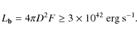
|
(2) |
This luminosity is several orders of magnitude larger than that of the bursts of the AXPs observed up to now (see Table 1). At the same time, the luminosity of the bursts of 1E 1547.0-5408 turns out to be comparable to the one of a typical SGR burst (see e.g. Mereghetti 2008).
The short initial spike of burst b is less pronounced in the ISGRI lightcurves. This might be due to the fact that in spite of the significant absorption of the signal from the source by the walls of the IBIS telescope, the signal in the ISGRI detector is strongly affected by saturation effects, while in the ACS detector the saturation is less pronounced. Otherwise, the difference in the strength of the spike in the ISGRI and ACS lightcurves could be due to the hardness of the spectrum of the spike. A ``hard spike plus soft extended tail'' morphology is typical for the SGR bursts (Gögüs et al. 2001; see, however, Ref. Ibrahim et al. 2001, who report a powerful SGR burst with a pulsating tail but without hard onset spike).
Table 1: Comparison of peak fluxes and luminosities of the AXP bursts.
![\begin{figure}
\par\includegraphics[width=18cm]{11988fig3.eps}
\end{figure}](/articles/aa/full_html/2010/02/aa11988-09/img54.png)
|
Figure 3:
The lightcurves of the bursts marked as ac) and d) in Fig. 2.
Red solid (black dotted) line shows the ISGRI detector lightcurve in
the 20-60 keV (60-200 keV) energy band, binned in 50 ms
time bins. The periods of zero count rate correspond to the gaps which
occurred because of the telemetry saturation. Blue dashed blue line
shows the SPI/ACS lightcurve. Signal oscillations visible in the long
burst c are with the period |
| Open with DEXTER | |
The two possibilities can be, in principle, distinguished via an analysis of the hardness ratio in the ISGRI detector alone. Indeed, the soft (20-60 keV) and hard (60-200 keV) band fluxes in ISGRI should be affected by saturation effects in a similar way, so that the hardness ratio does not change. The middle panels of Fig. 3 show the evolution of the ISGRI hardness ratio over the four brightest bursts. One can see that the spikes of the bursts b and c indeed have somewhat harder spectra than the afterglows. However, the jump in the ACS/ISGRI hardness ratio during the spike is more pronounced than in the ISGRI/ISGRI hardness ratio. This indicates that both the above mentioned effects might be present: the spectrum of the spike is harder than the one of the afterglow and the signal in ISGRI is much stronger affected by the saturation effects than that in the ACS.
Not only the bright spike, but also the afterglow lightcurve of burst b
in the ISGRI detector suffers from a saturation effect, which is
visible as an anomaly in the distribution of waiting times between
subsequent photons. This saturation effect results in the production of
short time gaps of ![]() 16,
32 or 64 ms duration, which appear in a quasi-periodic manner. We
have corrected the ISGRI lightcurve shown in Fig. 3b
for this effect by excluding the gaps from the analysis. We have
checked that this photon counting problem affects only the brightest
burst and that no anomalies of the waiting times between subsequent
photons are present in the spikes and afterglows of the other bursts.
16,
32 or 64 ms duration, which appear in a quasi-periodic manner. We
have corrected the ISGRI lightcurve shown in Fig. 3b
for this effect by excluding the gaps from the analysis. We have
checked that this photon counting problem affects only the brightest
burst and that no anomalies of the waiting times between subsequent
photons are present in the spikes and afterglows of the other bursts.
The 100 ms burst phase of the brightest event is followed
by a softer ``afterglow'' tail which is characterized by a power-law
decay profile
![]() with
with
![]() ms for the ACS and ISGRI 60-200 keV energy band and
ms for the ACS and ISGRI 60-200 keV energy band and
![]() ms in the ISGRI 20-60 keV energy band. The powerlaw decay ends abruptly
ms in the ISGRI 20-60 keV energy band. The powerlaw decay ends abruptly ![]() 1 s
after the start of the burst, which might indicate a more complicated
behavior of the afterglow emission, e.g. the presence of pulsations
(see below).
1 s
after the start of the burst, which might indicate a more complicated
behavior of the afterglow emission, e.g. the presence of pulsations
(see below).
A somewhat weaker burst shown in Fig. 3c exhibits a spike plus afterglow morphology similar to the one of burst b,
but with a much larger fraction of the power emitted during the
afterglow phase. Two gaps in the ISGRI detector light curve appear
because of the telemetry saturation. This prevents an analysis of the
spectral evolution during the afterglow phase, but, as one can see from
the lower panel of Fig. 3c,
the ISGRI count rate closely follows the ACS count rate, so that the
hardness ratio does not change over the time interval where ISGRI data
are available. In the ACS lightcurve of the burst, shown by the blue
dashed line, one can clearly identify the oscillations with the period ![]() 2 s, close to the period of rotation of the neutron star. These oscillations were previously reported by Mereghetti et al. (2009b).
2 s, close to the period of rotation of the neutron star. These oscillations were previously reported by Mereghetti et al. (2009b).
The burst d shown in the Fig. 3d consists of a single hard spike of the duration of ![]() 100 ms,
with almost no detectable afterglow. The ratio of the peak luminosity
of the spike to the peak luminosity of the afterglow in this burst and
the hardness of the spike emission are comparable to the one of the
strongest burst b.
100 ms,
with almost no detectable afterglow. The ratio of the peak luminosity
of the spike to the peak luminosity of the afterglow in this burst and
the hardness of the spike emission are comparable to the one of the
strongest burst b.
3.3 Statistical study of the burst properties
![\begin{figure}
\par\includegraphics[width=9cm]{11988fig4.eps}
\end{figure}](/articles/aa/full_html/2010/02/aa11988-09/img58.png)
|
Figure 4: Hardness as a function of ACS count rate during the main activity period of the source shown in Fig. 2. |
| Open with DEXTER | |
From Fig. 3 it is clear that the bright short spikes in the burst lightcurves are characterized by comparable ACS/ISGRI hardness ratios. It is not clear a priori if all the short spikes have comparably hard spectra, independent of their strength, or whether the hardness ratio of the spike/afterglow emission is determined by the burst luminosity. In order to distinguish between these two possibilities, we plot in Fig. 4 the hardness ratio as a function of the ACS count rate during the main activity period. From this figure one can see a correlation between the hardness and the count rate, which indicates that brighter bursts and afterglows also tend to have harder spectra. The value of the hardness of the brightest bursts is affected by the saturation effects in ISGRI and possibly also in the ACS detectors, but for the moderate flux values the observed flux-hardness correlation is robust. The dependence of the hardness of the spectrum on the luminosity was noticed in the bursts of 1E 2259+586 by (Gavriil et al. 2004). This type of dependence is the opposite of those observed in SGR bursts, for which a softening of the spectrum with increasing luminosity was observed (Gögüs et al. 2001).
![\begin{figure}
\par\includegraphics[width=9cm]{11988fig5.eps}
\end{figure}](/articles/aa/full_html/2010/02/aa11988-09/img59.png)
|
Figure 5: Burst duration as a function of the ACS peak rate ( top panel) and fluence ( botttom panel). Solid lines show the powerlaw fits to the data points. The error of the burst duration is assumed to be equal to the size of the ACS lightcurve time bin, 50 ms. Points shown as lower limits on the flux/fluence are those affected by possible saturation effects in ACS detector. |
| Open with DEXTER | |
Figure 5 shows
the dependence of the burst duration on the peak count rate and overall
fluence of the bursts in ACS. The burst duration is defined as the time
interval between the start and end of the burst, defined as explained
in Sect. 2. In our case this duration measure is equivalent to the
so-called ``T90'' (the duration of time interval in
which 90% of the burst fluence is contained). This is explained by the
fact that signal statistics in ACS are very high for all the bursts
retained for the statistical analysis. It is clear that if a
significant fraction of the burst fluence is emitted in the extended
afterglow, a correlation between the burst duration and the fluence is
expected, because the afterglows of stronger bursts remain detectable
during longer periods of time. On the other hand, if most of the burst
fluence is emitted in a short spike, no correlation between the burst
duration and the fluence would be present. Figure 5
indicates that in most of the bursts a significant contribution to the
total energy output comes from the afterglow emission. On the other
hand, one can see that the burst duration T is correlated with
the peak flux, i.e. bursts with stronger spikes possess on average
stronger afterglows. If the correlation of the burst durations with
burst fluxes and fluences are fit by power law, the best-fit powerlaw
dependences are
![]() and
and
![]() for the peak flux and fluence respectively. It is clear from Fig. 4 that the spread of the data points around the powerlaw model fit is quite large, which explains the very high reduced
for the peak flux and fluence respectively. It is clear from Fig. 4 that the spread of the data points around the powerlaw model fit is quite large, which explains the very high reduced
![]() values of the fit of the peak flux vs. duration correlation,
values of the fit of the peak flux vs. duration correlation,
![]() (for 82 d.o.f.). The fluence vs. duration correlation is somewhat
tighter and the quality of the powerlaw fit is somewhat better,
(for 82 d.o.f.). The fluence vs. duration correlation is somewhat
tighter and the quality of the powerlaw fit is somewhat better,
![]() (for 82 d.o.f.). The observed fluence-duration correlation is different from the one observed in 1E 2259+586 (
(for 82 d.o.f.). The observed fluence-duration correlation is different from the one observed in 1E 2259+586 (
![]() by Gavriil et al. 2004) and instead resembles more the fluence-duration relation of SGR bursts, e.g.
by Gavriil et al. 2004) and instead resembles more the fluence-duration relation of SGR bursts, e.g.
![]() in SGR 1900+14, (Gögüs et al. 1999) (note that the correlation F-T correlation is not very tight both in our case and in the case of SGR 1900+14, so that the two relations are consistent).
in SGR 1900+14, (Gögüs et al. 1999) (note that the correlation F-T correlation is not very tight both in our case and in the case of SGR 1900+14, so that the two relations are consistent).
From Fig. 3 it is clear that already in the forth-brightest burst d
the afterglow emission is difficult to detect because of the much lower
signal statistics. This means that for most of the weaker bursts,
visible in Fig. 2, only the bright spike is detectable. The duration of the spikes in the bursts b, c and d shown in Fig. 3 is 1-2 ACS time bins, i.e. ![]() 100 ms. One expects that the
100 ms. One expects that the ![]() 100 ms
spike duration should give a correct estimate of the typical durations
of the majority of the weaker bursts detected by the ACS during the
activity of the source. This is confirmed by Fig. 6
in which the distribution of durations of the bursts detected
simultaneously by the ACS and ISGRI detectors is shown, peaking at
100 ms. The 50 ms time resolution of the ACS detector does
not allow the measurement of details of the burst duration distribution
on shorter time scales. Fitting the distribution of burst durations
with a log-normal distribution we find a mean of
100 ms
spike duration should give a correct estimate of the typical durations
of the majority of the weaker bursts detected by the ACS during the
activity of the source. This is confirmed by Fig. 6
in which the distribution of durations of the bursts detected
simultaneously by the ACS and ISGRI detectors is shown, peaking at
100 ms. The 50 ms time resolution of the ACS detector does
not allow the measurement of details of the burst duration distribution
on shorter time scales. Fitting the distribution of burst durations
with a log-normal distribution we find a mean of
![]() ms and a scatter of 30 ms <T<155 ms.
The excess of longer duration bursts in the 0.5-10 s interval is
due to the presence of the extended afterglows and of several
``plateau'' like events, similar to burst a shown in Fig. 3a.
ms and a scatter of 30 ms <T<155 ms.
The excess of longer duration bursts in the 0.5-10 s interval is
due to the presence of the extended afterglows and of several
``plateau'' like events, similar to burst a shown in Fig. 3a.
![\begin{figure}
\par\includegraphics[width=9cm]{11988fig6.eps}
\end{figure}](/articles/aa/full_html/2010/02/aa11988-09/img68.png)
|
Figure 6: Distribution of burst durations in ACS. Thin solid curve shows the best fit log normal distribution. |
| Open with DEXTER | |
From the bottom panel of Fig. 1
it is clear that the main activity period of the source is
characterized by the extremely short intervals between subsequent
bursts. The waiting time decreases down to values comparable to the
burst durations at the peak of activity. Figure 7
shows the distribution of waiting times between the bursts for the
entire activity period on 22 January 2009. The waiting time
distribution can be fit by a wide log-normal distribution with a mean
![]() s and a scatter of
s and a scatter of
![]() s.
At the peak of activity, the waiting time between subsequent bursts
decreases to a time scale comparable to the duration of individual
spikes, so that the bursts can be considered as either separate events
or as parts of the ``multi-spike'' flares. This behavior is similar to
the one observed in SGR bursts (Gögüs et al. 1999). At the same time, the observed scatter of the waiting times is larger than the one found in the RXTE observations of 1E 2259+586 by Gavriil et al. (2004), who found that the waiting time between subsequent bursts is always larger than 1 s (
s.
At the peak of activity, the waiting time between subsequent bursts
decreases to a time scale comparable to the duration of individual
spikes, so that the bursts can be considered as either separate events
or as parts of the ``multi-spike'' flares. This behavior is similar to
the one observed in SGR bursts (Gögüs et al. 1999). At the same time, the observed scatter of the waiting times is larger than the one found in the RXTE observations of 1E 2259+586 by Gavriil et al. (2004), who found that the waiting time between subsequent bursts is always larger than 1 s (![]() 10
times longer than the typical burst duration). The difference between
the minimal waiting times between subsequent bursts in 1E 1547.0-5408,
reported here, and that of the bursts of 1E 2259+586, reported by Gavriil et al. (2004), could have four different explanations:
10
times longer than the typical burst duration). The difference between
the minimal waiting times between subsequent bursts in 1E 1547.0-5408,
reported here, and that of the bursts of 1E 2259+586, reported by Gavriil et al. (2004), could have four different explanations:
- 1.
- the bursts of 1E 2259+586 and of 1E 1547.0-5408 are physically different;
- 2.
- the RXTE observations of 1E 2259+586 missed the peak of the bursting activity of the source;
- 3.
- a gap between the minimal waiting time and burst duration in the 1E 2259+586 observations is related to the sensitivity limit of RXTE (weaker bursts remained undetected);
- 4.
- the definition of ``burst event'' used by Gavriil et al. (2004) slightly differs from the one used in our analysis
![[*]](/icons/foot_motif.png) .
.
![\begin{figure}
\par\includegraphics[width=9cm]{11988fig7.eps}
\end{figure}](/articles/aa/full_html/2010/02/aa11988-09/img72.png)
|
Figure 7: Distribution of the waiting times between subsequent bursts. |
| Open with DEXTER | |
The arrival times of bursts of AXPs are found to be correlated with the pulsed emission phase. In the case of 1E 1547.0-5408 this fact is difficult to verify, because the amplitude of the pulsed quiescent X-ray emission is just some 7% of the quiescent X-ray flux (Halpern et al. 2008). It is clear from Fig. 3c that the amplitude of the pulsed emission significantly increases during the afterglows of the bright bursts. To test if the arrival times of the individual bursts are correlated with the phase of the pulsed radio/X-ray emission, one can
- study the distribution of the phases of arrival of the short spikes and/or;
- compare the phases of the maxima of the pulsed tails of the brightest bursts.
Figure 8 shows a comparison of the afterglows of three bright bursts. The burst shown by the solid line is the brightest burst b, the burst shown by the dashed line is the second brightest burst c
and the burst shown by the dotted line is a somewhat weaker burst,
which happened two hours after the main activity episode. To shift the
lightcurves of the individual bursts by an integer number of periods,
we use the measurement of the period of 1E 1547.0-5408 reported by Kuiper et al. (2009).
From this figure one can notice that although the phases of the maxima
of the pulsed afterglow do not coincide exactly, they are rather close
to each other. If the afterglow is due to emission from the surface of
the neutron star, this might indicate that the afterglows of different
bursts are produced by one and the same ``hot spot'' on the neutron
star's surface or that the ``trapped fireball'' in the neutron star's
magnetosphere always appears at the same latitude/longitude. For
comparison, we show in the same figure the ACS lightcurve of the
brightest burst b. The phase of the sharp end of the afterglow of burst b is shifted by
![]() with respect to the phases of the maxima of the pulsed afterglow
emission of the other bursts. If the sharpness of the termination of
the afterglow of burst b
is ascribed to the presence of pulsations in the afterglow emission,
the location of the afterglow-emitting region of this burst should be
displaced. Otherwise, the difference in the strength and shift in the
phase between the afterglows of the bursts b and c could be due to different physical mechanisms of the afterglow production.
with respect to the phases of the maxima of the pulsed afterglow
emission of the other bursts. If the sharpness of the termination of
the afterglow of burst b
is ascribed to the presence of pulsations in the afterglow emission,
the location of the afterglow-emitting region of this burst should be
displaced. Otherwise, the difference in the strength and shift in the
phase between the afterglows of the bursts b and c could be due to different physical mechanisms of the afterglow production.
From Fig. 8
one can notice that, contrary to the pulsed afterglows, the short
spikes of different bursts do not arrive in phase. This is confirmed by
Fig. 9, which shows the distribution of the number of bursts as a function of the phase of the pulsed emission. The phase ![]() is assumed to be the phase of the sharp end of the afterglow of burst b. One can see that the phases of the bright spikes are randomly distributed over the pulse period.
is assumed to be the phase of the sharp end of the afterglow of burst b. One can see that the phases of the bright spikes are randomly distributed over the pulse period.
It is worth noting that the short spikes indeed seem to arrive at random times and that properties (flux, arrival time) of the spike are not correlated with the properties of the afterglows. For example, the burst shown by the green dotted line in Fig. 8 has a sharp start of the afterglow, but does not possess an initial spike at all. We have also found bursts in which the moment of arrival of the short spike is delayed compared to the moment of the onset of the ``afterglow-like'' emission.
![\begin{figure}
\par\includegraphics[width=9cm]{11988fig8.eps}
\end{figure}](/articles/aa/full_html/2010/02/aa11988-09/img76.png)
|
Figure 8:
Relative phases of the pulses of the burst afterglows. The green dotted
line shows a bust which occurred on January 22, 8:18 am. Black solid
line shows the brightest burst b shifted by 2671 periods forward in time. The blue dashed line shows the second-brightest burst c
shifted by 2589 periods. The count rate of this burst is multiplied by
a factor of three to highlight the similarity with the time profile of
the burst c. The vertical solid and dashed line shows the
phases of the maxima of the pulses of the burst afterglows. The
vertical solid lines are shifted by
|
| Open with DEXTER | |
![\begin{figure}
\par\includegraphics[width=9cm]{11988fig9.eps}
\end{figure}](/articles/aa/full_html/2010/02/aa11988-09/img77.png)
|
Figure 9: Distribution of the burst start times in terms of the phase of the pulsed emission. |
| Open with DEXTER | |
The large effective area of the ACS detector enables us to detect the
bursts with a fluence down to three orders of magnitude lower than the
one of the brightest bursts. The distribution of the burst fluences is
shown in Fig. 10. The fluence distribution follows a power law with an exponent
![]() over a dynamic range of
over a dynamic range of ![]() 3 decades in fluence. This behavior is similar to the one observed in the SGR bursts (Gögüs et al. 1999).
Deviation from the power-law behaviour at the low flux / fluence end of
the distribution is due to the limited sensitivity of the ISGRI
detector: the weaker bursts visible in the ACS fall below the
3 decades in fluence. This behavior is similar to the one observed in the SGR bursts (Gögüs et al. 1999).
Deviation from the power-law behaviour at the low flux / fluence end of
the distribution is due to the limited sensitivity of the ISGRI
detector: the weaker bursts visible in the ACS fall below the ![]() significance threshold which we have adopted for the burst selection in
ISGRI. It is interesting to note that if the luminosities of the
brightest bursts from 1E 1547.0-5408 are
significance threshold which we have adopted for the burst selection in
ISGRI. It is interesting to note that if the luminosities of the
brightest bursts from 1E 1547.0-5408 are ![]() 1042 erg s-1, the weakest bursts included in our analysis have luminosities
1042 erg s-1, the weakest bursts included in our analysis have luminosities ![]() 1039 erg s-1,
matching the luminosity of the brightest burst from AXPs detected
before. Comparing the distribution of the burst fluences in 1E
1547.0-5408 with the one of 1E 2259+586 (Gavriil et al. 2004), we find that in spite of significant differences in the luminosity of individual bursts (
1039 erg s-1,
matching the luminosity of the brightest burst from AXPs detected
before. Comparing the distribution of the burst fluences in 1E
1547.0-5408 with the one of 1E 2259+586 (Gavriil et al. 2004), we find that in spite of significant differences in the luminosity of individual bursts (![]() 1039 erg s-1 in 1E 2259+586 vs.
1039 erg s-1 in 1E 2259+586 vs. ![]() 1042 erg s-1 in 1E 1547.0-5408), both distributions have a power-law shape with approximately the same slopes (
1042 erg s-1 in 1E 1547.0-5408), both distributions have a power-law shape with approximately the same slopes (
![]() in the case of 1E 2259+586 vs.
in the case of 1E 2259+586 vs.
![]() in 1E 1547.0-5408). This indicates that the observed power-law behavior
of the distribution of burst strengths should be valid also for the
weaker bursts which are below the ISGRI detection limit. The
distribution of the burst peak count rates, shown in the top panel of
Fig. 10 has a smaller dynamical range. A powerlaw fit of this distribution, shown in the same panel, is characterized by a slope of
in 1E 1547.0-5408). This indicates that the observed power-law behavior
of the distribution of burst strengths should be valid also for the
weaker bursts which are below the ISGRI detection limit. The
distribution of the burst peak count rates, shown in the top panel of
Fig. 10 has a smaller dynamical range. A powerlaw fit of this distribution, shown in the same panel, is characterized by a slope of
![]() ,
flatter than that of the distribution of the burst fluxes in 1E 2259+586,
,
flatter than that of the distribution of the burst fluxes in 1E 2259+586,
![]() .
.
![\begin{figure}
\par\includegraphics[width=9cm]{11988fig10.eps}
\end{figure}](/articles/aa/full_html/2010/02/aa11988-09/img83.png)
|
Figure 10: Top panel: distribution of the ACS peak count rates of the bursts detected by both ACS and ISGRI detectors. Bottom panel: distribution of fluences of the bursts. The thin straight lines show powerlaw fits to the distributions. |
| Open with DEXTER | |
4 Discussion and conclusions
We have studied an exceptional period of activity of 1E 1547.0-5408 which occurred on 22 January 2009. During this activity period, about 200 bursts were detected by SPI/ACS and 84 of them were also detected by IBIS/ISGRI detector. The luminosity of the brightest of these bursts was comparable to the luminosity of the SGR bursts and/or giant flares. This is the first time that bursts of such strength are registered from an AXP. In spite of the fact that the source was outside of the field of view of the INTEGRAL instruments, we were able to study spectral and temporal characteristics of the bursts, because the signal was so strong that in spite of significant attenuation it was able to penetrate through the walls of the IBIS imager.
We have found that the activity of the source has exponentially
increased on the time scale of about one hour, reaching a peak at
around UTC 2009-22-01T06:40. The maximum of the activity was
characterized by a very high rate of bursts from the source, with the
minimum of the waiting time between subsequent bursts reaching
0.2 s, which is comparable to the typical burst duration. The
increase of the burst rate was accompanied by an increase of the
strength of the individual bursts. We were not able to measure the flux
of the brightest bursts because of saturation effects. However, we
estimate the lower limit on the peak luminosity of the brightest burst
to be
![]() erg s-1.
This luminosity is several orders of magnitude larger than that of the
previously detected bursts from other AXPs. Our study of the
statistical properties of the large amount of the 1E 1547.0-5408 bursts
reveals that the typical duration of the bursts is
erg s-1.
This luminosity is several orders of magnitude larger than that of the
previously detected bursts from other AXPs. Our study of the
statistical properties of the large amount of the 1E 1547.0-5408 bursts
reveals that the typical duration of the bursts is ![]() 100 ms. The distribution of the burst duration extends to
100 ms. The distribution of the burst duration extends to ![]() 10 s, see Fig. 6.
The typical and maximal burst durations correspond to the time scales
of the short spikes and of the extended afterglows of individual
bursts. We find that brighter bursts are characterized by longer
durations (Fig. 5) and by harder spectra (Fig. 4).
The extended afterglows of the brightest bursts exhibit pulsations with
a period equal to the rotation period of the neutron star. The phases
of the maxima of the pulsed afterglow emission of different bursts are
close to each other, which indicates that the region (a ``trapped
fireball'' in the magnetosphere, or a ``hot spot'' on the neutron star
surface) is located at the same place in different bursts. At the same
time, the bright short spikes of different bursts do not tend to arrive
at a preferred phase, which might indicate that the spikes are not
produced in the same region as the afterglow emission, as it is
expected e.g. in the magnetic reconnection model, in which the bursts
occur at high altitudes in the magnetosphere (Lyutikov 2002).
Otherwise, the absence of a correlation with the phase of the pulsed
tail emission could be explained by the fact that the emission of the
bright spikes is relativistically beamed. The beaming effects might
also explain the presence of the ``orphan'' afterglows without spikes
and the time delays between the onset of the afterglow and the spike
arrival time, observed in a number of 1E 1547.0-5408 bursts.
10 s, see Fig. 6.
The typical and maximal burst durations correspond to the time scales
of the short spikes and of the extended afterglows of individual
bursts. We find that brighter bursts are characterized by longer
durations (Fig. 5) and by harder spectra (Fig. 4).
The extended afterglows of the brightest bursts exhibit pulsations with
a period equal to the rotation period of the neutron star. The phases
of the maxima of the pulsed afterglow emission of different bursts are
close to each other, which indicates that the region (a ``trapped
fireball'' in the magnetosphere, or a ``hot spot'' on the neutron star
surface) is located at the same place in different bursts. At the same
time, the bright short spikes of different bursts do not tend to arrive
at a preferred phase, which might indicate that the spikes are not
produced in the same region as the afterglow emission, as it is
expected e.g. in the magnetic reconnection model, in which the bursts
occur at high altitudes in the magnetosphere (Lyutikov 2002).
Otherwise, the absence of a correlation with the phase of the pulsed
tail emission could be explained by the fact that the emission of the
bright spikes is relativistically beamed. The beaming effects might
also explain the presence of the ``orphan'' afterglows without spikes
and the time delays between the onset of the afterglow and the spike
arrival time, observed in a number of 1E 1547.0-5408 bursts.
A consistent interpretation of the burst timing and spectral properties observed in the 22 January 2009 activity episode of 1E 1547.0-5408 within the two main models of the magnetar flares, the ``crustal fracture'' and the ``magnetic reconnection'' models (Thompson & Duncan 1995; Lyutikov 2002), requires further theoretical investigation. It is not clear if the large variety of burst morphologies (which might be somewhat broader than the ``type A/B'' classification introduced by Woods et al. 2005) could be explained within one of the two mechanisms. In spite of the comparable luminosity, it is also not clear if the mechanism of production of the 1E 1547.0-5408 bursts is the same as that of the SGR bursts.
Observation of SGR-like bursts from an AXP adds additional argument in favor of the hypothesis that AXPs and SGRs form a unique source population, so that 1E 1547.0-5408 is an ``intermediate'' AXP/SGR representative of this population. Indeed, persistent X-ray emission of 1E 1547.0-5408 is characterized by typical AXP spectral characteristics (Halpern et al. 2008). At the same time 1E 1547.0-5408 is distinguished from other AXPs by the presence of pulsed radio emission (Camilo et al. 2007), which was otherwise only observed in the case of AXP XTE J1810-197 (Camilo et al. 2006). At the same time, contrary to most of the SGRs, it appears to have a clear supernova remnant association (Gelfand & Gaeinsler 2007). Presence of the ``various faces'' (radio pulsar/AXP/SGR) in various states of 1E 1547.0-5408 demonstrates that observational properties of AXPs and SGRs are determined by the same physical mechanisms.
AcknowledgementsWe would like to thank W. Collmar for providing us with access to the ISGRI data for the period of activity of 1E 1547.0-5408.
References
- Baldovin, C., Savchenko, V., Beckmann, V., et al. 2009, ATEL, 1908 [Google Scholar]
- Burgay, N., Israel, G. L., Possenti, A., et al. 2009, ATEL, 1913 [Google Scholar]
- Camilo, F., Ransom, S. M., Halpern, J. P., et al. 2006, Nature, 442, 892 [NASA ADS] [CrossRef] [PubMed] [Google Scholar]
- Camilo, F., Ransom, S. M., Halpern, J. P., & Reynolds, J. 2007, ApJ, 666, L93 [NASA ADS] [CrossRef] [Google Scholar]
- Camilo, F., Halpern, J. P., & Ransom, S. M. 2009, ATEL, 1907 [Google Scholar]
- Connaughton, V., & Briggs, M. 2009, GCN, 8835 [Google Scholar]
- Courvoisier, T. J.-L., Walter, R., Beckmann, V., et al. 2003, A&A, 411, L53 [NASA ADS] [CrossRef] [EDP Sciences] [Google Scholar]
- den Hartog, P. R., Kuiper, L., & Hermsen, W. 2009, ATEL 1922 [Google Scholar]
- Dib R., Kaspi, V. M., & Gavriil, F. P. 2008, [arXiv:0811.2659] [Google Scholar]
- Duncan, R. C., & Thompson, C. 1992, ApJ, 392, L9 [NASA ADS] [CrossRef] [Google Scholar]
- Gavriil, F. P., Kaspi, V. M., & Woods P. M. 2002, Nature, 419, 142 [NASA ADS] [CrossRef] [PubMed] [Google Scholar]
- Gavriil, F. P., Kaspi, V. M., & Woods P. M. 2004, ApJ, 607, 959 [NASA ADS] [CrossRef] [Google Scholar]
- Gavriil, F. P., Dib, R., & Kaspi, V. M. 2008, in 40 Years of Pulsars: Millisecond Pulsars, Magnetars and More, AIP Conf. Proc., [arXiv:0712.4186] [Google Scholar]
- Gelfand, J. D., & Gaensler, B. M. 2007, ApJ, 667, 1111 [NASA ADS] [CrossRef] [Google Scholar]
- Gögüs, E., Woods, P. M., Kouveliotou, C., et al. 1999, ApJ, 526, L93 [NASA ADS] [CrossRef] [PubMed] [Google Scholar]
- Gögüs, E., Kouveliotou, C., Woods, P. M., et al. 2001, ApJ, 558, 228 [NASA ADS] [CrossRef] [Google Scholar]
- Golenetskii, S., Aptekar, R., Mazets, E., et al. 2009, GCN 8913 [Google Scholar]
- Götz D., Mereghetti, S., Tiengo, A., & Esposito, P. 2006, A&A, 449, L31 [NASA ADS] [CrossRef] [EDP Sciences] [Google Scholar]
- Gronwall, C., Holland, S. T., Markwardt, C. B., et al. 2009, GCN, 8833 [Google Scholar]
- Halpern, J. P., Gotthelf, E. V., Reynolds, J., Ransom ,S. M., & Camilo F. 2008, ApJ, 676, 1178 [NASA ADS] [CrossRef] [Google Scholar]
- Hurley, K. J., McBreen, B., Rabbette, M., & Steel, S. 2004, A&A, 288, L49 [Google Scholar]
- Hurley, K., Boggs, S. E., Smith, D. M., et al. 2005, Nature, 434, 1098 [NASA ADS] [CrossRef] [PubMed] [Google Scholar]
- Israel, G. L., Campagna, S., Dall'Osso, S., et al. 2007, ApJ, 664, 448 [NASA ADS] [CrossRef] [Google Scholar]
- Ibrahim, A. I., Strohmayer, T. E., Woods, P. M., et al. ApJ, 558, 237 [Google Scholar]
- Kaspi, V. M., Gavriil, F. P., Woods, P. M., et al. 2003, ApJ, 588, L93 [NASA ADS] [CrossRef] [Google Scholar]
- Kouveliotou, C., von Kienlin, A., Fishman, G., et al., 2009, GCN, 8915 [Google Scholar]
- Kuiper, L., den Hartog, P. R., & Hermsen, W. 2009, ATEL, 1921 [Google Scholar]
- Lamb, R. C., & Markert, T. H. 1981, ApJ, 244, 94 [NASA ADS] [CrossRef] [Google Scholar]
- Lebrun, F., Leray, J. P., Lavocat, P., et al. 2003, A&A, 411, L141 [NASA ADS] [CrossRef] [EDP Sciences] [Google Scholar]
- Lyutikov, M. 2002, ApJ, 580, L65 [NASA ADS] [CrossRef] [Google Scholar]
- Marcinkowski, R., Denis, M., Bulik, T., et al. 2006, A&A, 452, 113 [NASA ADS] [CrossRef] [EDP Sciences] [Google Scholar]
- Mereghetti, S. 2008, A&ARv, 15, 225 [NASA ADS] [CrossRef] [Google Scholar]
- Mereghetti, S., Götz, D., von Kienlin, A., et al. 2005, ApJ, 624, L105 [NASA ADS] [CrossRef] [Google Scholar]
- Mereghetti, S., Götz, D., Weidenspointner, G., et al. 2009a, ApJ, 696, L74 [NASA ADS] [CrossRef] [Google Scholar]
- Mereghetti, S., Gotz, D., von Kienlin, A., et al. 2009b, GCN, 8841 [Google Scholar]
- Paczynski, B. 1992, Acta Astron., 42, 145 [NASA ADS] [Google Scholar]
- Savchenko, V., Beckmann, V., Neronov, A., et al. 2009, GCN, 8837 [Google Scholar]
- Thompson, C., & Duncan, R. C. 1995, MNRAS, 275, 255 [NASA ADS] [CrossRef] [Google Scholar]
- von Kienlin, A., & Connaughton, V. 2009, GCN, 8838 [Google Scholar]
- von Kienlin, A., Beckmann, V., Rau, A., et al. 2003, A&A, 411, L299 [NASA ADS] [CrossRef] [EDP Sciences] [Google Scholar]
- Winkler, C., Courvoisier, T. J.-L., Di Cocco, G., et al. 2003, A&A, 411, L1 [NASA ADS] [CrossRef] [EDP Sciences] [Google Scholar]
- Woods, P. M., Kouveliotou, C., Gavriil, F. P., et al. 2005, ApJ, 629, 985 [NASA ADS] [CrossRef] [Google Scholar]
Footnotes
- ... barycent
- barycent tool is a part of the INTEGRAL Offline Science Analysis (OSA) package distributed by ISDC (Courvoisier et al. 2003). tool and substituting the source coordinates found by Camilo et al. (2007).
- ... flux
- The analysis of Mereghetti et al. (2009a), which appeared after this paper was submitted, results in a comparable estimate of the lower limit on the source flux.
- ... analysis
- E.g. two individual bursts with short waiting time
 s
might have been considered as a single multi-peaked burst in the
analysis of Gavriil
et al.
(2004).
s
might have been considered as a single multi-peaked burst in the
analysis of Gavriil
et al.
(2004).
All Tables
Table 1: Comparison of peak fluxes and luminosities of the AXP bursts.
All Figures
|
|
Figure 1:
Top: the thick solid line is the rate of bursts detected both
in IBIS/ISGRI and SPI/ACS as a function of time on 22 January 2009. The
dashed blue histogram shows the cumulative burst distribution. The thin
straight solid historgam shows a fit with an exponentially rising burst
rate with rise time
|
| Open with DEXTER | |
| In the text | |
|
|
Figure 2: SPI/ACS lightcurve during the main activity episode of 1E 1547.0-5408 between 6:30 and 7:00, 22 January 2009 (UTC). |
| Open with DEXTER | |
| In the text | |
|
|
Figure 3:
The lightcurves of the bursts marked as ac) and d) in Fig. 2.
Red solid (black dotted) line shows the ISGRI detector lightcurve in
the 20-60 keV (60-200 keV) energy band, binned in 50 ms
time bins. The periods of zero count rate correspond to the gaps which
occurred because of the telemetry saturation. Blue dashed blue line
shows the SPI/ACS lightcurve. Signal oscillations visible in the long
burst c are with the period |
| Open with DEXTER | |
| In the text | |
|
|
Figure 4: Hardness as a function of ACS count rate during the main activity period of the source shown in Fig. 2. |
| Open with DEXTER | |
| In the text | |
|
|
Figure 5: Burst duration as a function of the ACS peak rate ( top panel) and fluence ( botttom panel). Solid lines show the powerlaw fits to the data points. The error of the burst duration is assumed to be equal to the size of the ACS lightcurve time bin, 50 ms. Points shown as lower limits on the flux/fluence are those affected by possible saturation effects in ACS detector. |
| Open with DEXTER | |
| In the text | |
|
|
Figure 6: Distribution of burst durations in ACS. Thin solid curve shows the best fit log normal distribution. |
| Open with DEXTER | |
| In the text | |
|
|
Figure 7: Distribution of the waiting times between subsequent bursts. |
| Open with DEXTER | |
| In the text | |
|
|
Figure 8:
Relative phases of the pulses of the burst afterglows. The green dotted
line shows a bust which occurred on January 22, 8:18 am. Black solid
line shows the brightest burst b shifted by 2671 periods forward in time. The blue dashed line shows the second-brightest burst c
shifted by 2589 periods. The count rate of this burst is multiplied by
a factor of three to highlight the similarity with the time profile of
the burst c. The vertical solid and dashed line shows the
phases of the maxima of the pulses of the burst afterglows. The
vertical solid lines are shifted by
|
| Open with DEXTER | |
| In the text | |
|
|
Figure 9: Distribution of the burst start times in terms of the phase of the pulsed emission. |
| Open with DEXTER | |
| In the text | |
|
|
Figure 10: Top panel: distribution of the ACS peak count rates of the bursts detected by both ACS and ISGRI detectors. Bottom panel: distribution of fluences of the bursts. The thin straight lines show powerlaw fits to the distributions. |
| Open with DEXTER | |
| In the text | |
Copyright ESO 2010
Current usage metrics show cumulative count of Article Views (full-text article views including HTML views, PDF and ePub downloads, according to the available data) and Abstracts Views on Vision4Press platform.
Data correspond to usage on the plateform after 2015. The current usage metrics is available 48-96 hours after online publication and is updated daily on week days.
Initial download of the metrics may take a while.