Properties of starspots on CoRoT-2

A. Silva-Valio; A. F. Lanza; R. Alonso; P. Barge

doi:10.1051/0004-6361/200911904

Home

All issues

Volume 510 (February 2010)

A&A, 510 (2010) A25

Full HTML

Free Access

Issue		A&A Volume 510, February 2010


Article Number		A25
Number of page(s)		6
Section		Stellar atmospheres
DOI		https://doi.org/10.1051/0004-6361/200911904
Published online		02 February 2010

A&A 510, A25 (2010)

Properties of starspots on CoRoT-2

A. Silva-Valio¹ - A. F. Lanza² - R. Alonso³ - P. Barge³

1 - CRAAM, Mackenzie University, Rua da Consolação, 896, 01302-907, São Paulo, Brazil
2 - INAF-Osservatorio Astrofisico di Catania, via S. Sofia, 78, 95123 Catania, Italy
3 - Laboratoire d'Astrophysique de Marseille, UMR 6110, CNRS/Université de Provence, Traverse du Siphon, 13376 Marseille, France

Received 20 February 2009 / Accepted 9 November 2009

Abstract
Context. As a planet eclipses its parent star, a dark spot on the surface of the star may be occulted, causing a detectable variation in the light curve.
Aims. We study these light curve variations during transits and infer the physical characteristics of the stellar spots.
Methods. A total of 77 consecutive transit light curves of CoRoT-2 were observed with a high temporal resolution of 32 s, corresponding to an uninterrupted period of 134 days. By analyzing small intensity variations in the transit light curves, it was possible to detect and characterize spots on the surface of the star. The model used simulates planetary transits and enables the inclusion of spots on the stellar surface with different sizes, intensities (i.e., temperatures), and positions. Fitting the data with this model, it is possible to infer the physical characteristics of the spots. Because what is observed is the stellar flux blocked by the spots, there is a degeneracy between the spot intensity and area, although the spot radius defines the shape and width of the signal in the light curve. The model allows up to 9 spots to be present on the stellar surface within the transit band.
Results. Before the modeling of the spots was performed, the planetary radius relative to the star radius was estimated by fitting the deepest transit to minimize the effect of spots. A slightly larger (3%) radius, 0.172 $R_{\rm star}$ , resulted instead in the previously reported 0.1667 $R_{\rm star}$ . The fitting of the transits yields spots, or spot groups, of sizes ranging from 0.2 to 0.7 planetary radius, $R_{\rm p}$ , with a mean of $0.46 \pm 0.11\ R_{\rm p}$ ( ${\sim} 100~000$ km), resulting in a stellar area covered by spots within the transit latitudes of 10-20%. The intensity varied from 0.3 to 0.8 of the disk center intensity, $I_{\rm c}$ , with a mean of $0.55 \pm 0.13\ I_{\rm c}$ , which can be converted to temperature by assuming black-body emission for both the photosphere and the spots. Considering an effective temperature of 5625 K for the stellar photosphere, the mean spot temperature is $4700 \pm 300$ K.
Conclusions. The spot model used here was able to estimate the physical characteristics of the spots on CoRoT-2, such as size and intensity. The spots on CoRoT-2 are larger and cooler than sunspots, maybe confirming the more active nature of this star with respect to the Sun. The results presented here are in agreement with those found for magnetic activity analysis from out of transit data of the same star.

Key words: stars: activity - starspots - planetary systems

1 Introduction

Four centuries ago, spots on the surface of the Sun were first detected by Galileo. Sunspots are cool regions of strong concentrations of magnetic fields on the photosphere of the Sun. Presently, observations of unprecedented photometric precision by the CoRoT satellite (Baglin et al. 2006), have detected spots on the surface of another star, that of CoRoT-2, a far more active star. This activity is probably a consequence of its young age, estimated to be 0.5 Gyr (Bouchy et al. 2008). CoRoT-2 is one of 7 stars with transiting planets detected so far by CoRoT.

Spot activity has been inferred in the past from the modulation observed in the light of stars. As the star rotates, different spots on its surface are brought into view. Because spots are cooler, and therefore darker, than the surrounding photosphere, the detected total light of the star diminishes as different spots of varying temperature and size face the observer. This periodic modulation enables the determination of the rotation period of the star.

The magnetic activity of CoRoT-2 star was studied in detail by Lanza et al. (2009) who analyzed its out-of-transit light curve with modulations of $\sim$ 6% of its total flux. Using maximum entropy regularized models, Lanza et al. (2009) modeled the light curve considering both the presence of sunspots and faculae (dark and bright regions, respectively). This study detected two active longitudes located in opposite hemispheres, and also found that these longitudes varied with time. The active longitudes are regions where the spots preferably form. The total area covered by the spots were seen to vary periodically with a period of $29 \pm 4$ days. The authors were also able to estimate an amplitude for the relative differential rotation of ${\leq} 0.7$ %.

Wolter et al. (2009) modeled a single spot on the surface of CoRoT-2, obtaining the radius of the spot for a certain spot intensity. The authors pointed out the existing degeneracy between spot radius and intensity, because what is measured is the stellar flux deficit caused by the spot. Nevertheless, the characteristics of that single spot were a spot radius of 4.8 $^\circ$ (in degrees of stellar surface) for an intensity of 30% the star disk center value.

Here we propose to study the same spots on CoRoT-2, but with a different approach. A transiting planet can also be used as a probe of the contrasting features in the photosphere of the star. When the planet occults a dark spot on the surface of its host star, small variations in the light curve may be detected (Silva-Valio 2008; Silva 2003; Pont et al. 2007). By modeling these variations, the properties of starspots can be determined, such as size, position, and temperature. Moreover, from the continuous and long duration observations provided by the CoRoT satellite, the temporal evolution of individual spots can be obtained.

The next section describes the observation performed by CoRoT, whereas the model used here is introduced in the following section. The main results are presented in Sect. 4. Finally, a discussion of the main results and the conclusions are listed in Sect. 5.

2 Observation of CoRoT-2

A planet around the star CoRoT-2 was detected during one of the long-run observations of a field toward the Galactic center performed by the CoRoT satellite, and is the second transiting planet discovered. The planet, a hot Jupiter, with a mass of $3.3\ M_{\rm Jup}$ and radius of $1.47\ R_{\rm Jup}$ , orbits its host star in just 1.73 day (Alonso et al. 2008). CoRoT-2 is a solar-like star of type G7 with $0.97~M_\odot$ and 0.902 $R_\odot$ that rotates with a period of 4.54 days (Alonso et al. 2008). The parameters of the star and the planet, plus the orbital ones, were determined from a combination of CoRoT photometric light curve data (Alonso et al. 2008) and ground-based spectroscopy (Bouchy et al. 2008).

The data analyzed here were reduced following the same procedure as Alonso et al. (2008). The white light curve was filtered from cosmic ray impacts and orbital residuals. This cleaned light curve was then folded by considering an orbital period of 1.743 day, from which the parameters of the planetary system were derived. Besides the planet orbital period of $P_{\rm o} = 1.743$ day and stellar rotation of $P_{\rm s} = 4.54$ days, the orbital parameters were inferred semi-major axis of a = 6.7 star radius ( $R_{\rm s}$ ) and inclination angle of $87.84^\circ$ .

A total of 77 transits were detected in the light curve with a high temporal resolution of 32 s, for a total of 134 days. The rms of this signal was estimated from the out-of-transit data points to be $\sigma = 6\times 10^{-4}$ in relative flux units. Small brightness variations were detected during the transits, usually with fluxes of between 3 and $10 \sigma$ above the flux of the transit model without spots, the largest variation reaching $18 \sigma$ . These intensity variations were interpreted as the signatures of star spots and thus modeled. Figure 1 shows the light curves from all transits, where the vertical extent of each data point represents the rms of the signal. We also plot in this figure the model transit considering that no spots are present on the stellar surface (gray curves).

$\begin{figure} \par\includegraphics[width=9cm,clip]{11904fg1.eps} \vspace{4mm} \end{figure}$	Figure 1: All the 77 light curves during the transit of CoRoT-2b in front of its spotted host star. The gray solid line represent the model of a spotless star. The error bars of the data points indicate the rms of 0.0006.
Open with DEXTER

3 The model

The physical characteristics of star spots are obtained by fitting the model described in Silva (2003). In the model adopted here, the star is a 2D image of intensity that decreases following a quadratic limb darkening law according to Alonso et al. (2008), whereas the planet is assumed to be a dark disk. The modeled light curve of the transit is obtained as follows. The planet position in its orbit is calculated every two minutes and the total flux is just the sum of all pixels in the image (star plus dark planet). This yields the light curve, that is, the relative intensity as a function of time during the transit. The model assumes that the orbit is circular, that is, of null eccentricity (consistent with the measured eccentricity of $0.003 \pm 0.003$ ), and that the orbital plane is aligned with the stellar equator. In the case of CoRoT-2, the latter is a good assumption since, by measuring the Rossiter-McLaughlin effect, Bouchy et al. (2008) found that the angle between the stellar rotation axis and the normal to the orbital plane is only $7.2 \pm 4.5^\circ$ . The orbital parameters were taken from Alonso et al. (2008), such as a period of 1.743 day and an orbital radius of 6.7 $R_{\rm star}$ .

The model also allows the star to have features on its surface such as spots. The round spots are modeled by three parameters: (i) intensity, as a function of stellar intensity at disk center, $I_{\rm c}$ (maximum value); (ii) size, or radius, measured in units of planet radius, $R_{\rm p}$ ; and (iii) position or latitude (restricted to the transit path) and longitude. During all the fitting, the latitude of the spots remained fixed and equal to the planetary transit line, which for an inclination angle of $87.84^\circ$ is $-14.6^\circ$ . This latitude was arbitrarily chosen to be south, thus the minus sign. The longitude of the spot is measured with respect to the central meridian of the star, which coincides with the line-of-sight and the planet projection at transit center.

When the spot is close to the limb, the effect of foreshortening is also featured in the model. However, this model does not account for faculae. Solar-like faculae have negligible contrast close to the disk center, having significant contrast only close to the limb. Since the facular-to-spotted area ratio for CoRoT-2 is only Q = 1.5 (Lanza et al. 2009), instead of 9 as in the Sun, and we limit our analysis to spots between -70 and $+70^\circ$ from the central meridian, the photometric effect of faculae is very small and can be safely neglected.

The blocking of a spot by the planet during a transit implies an increase in the light detected, because a region darker than the stellar photosphere is being occulted. Thus the effect of many spots on the stellar surface is to decrease the depth of the transit, as can be seen in Fig. 1. This in turn will influence the determination of the planet radius, since a shallower transit depth results in a smaller estimate of the planet diameter when spots are ignored (Silva-Valio 2010).

In this work, to estimate the best-fit model parameters for the planet and its orbit, we searched for the deepest transit. Of all the 77 transits, the 32nd transit displays the smallest light variation (see Fig. 1). This was interpreted as the star with the minimum number of spots on its surface within the transit latitudes during the whole period of observation (134 days). The 32nd transit is shown in Fig. 2 as black crosses, for comparison, the fifth transit (gray crosses, red crosses in the color version) is also shown in the same figure.

$\begin{figure} \par\includegraphics[width=9cm,clip]{11904fg2.eps} \vspace*{-2mm} \end{figure}$

Figure 2:

Top: examples of transit light curves of CoRoT-2. The black crosses represent the 32nd transit assumed to occur when the star has minimum spot activity within the transit latitudes, whereas the gray (red crosses in the color version) data points represent a typical transit (the fifth one). The model light curve without any spots is shown as the thick solid curve. Bottom: residual from the subtraction of the data minus the model for a star with no spots for the 5th (gray/red) and 32nd (black) transits. The vertical bars in both panels represent the estimated uncertainty of 0.0006 from out of transit data.

Open with DEXTER

A light curve obtained from a model without any spot is shown as a thick solid curve on the figure. However, to obtain this model light curve it was necessary to use a planet radius of 0.172 stellar radius, instead of the 0.1667 stellar radius quoted in Table 1 of Alonso et al. (2008), which represents an increase of about 3%. We note that this may not be a difference in the true radius but rather an artifact due to the uneven spot coverage on the total surface of the star during that specific transit. Nevertheless, this implies that star spots can affect the exact size estimate of a planet by making the transit light curve shallower than it would otherwise be (Silva-Valio 2010).

$\begin{figure} \par\includegraphics[width=8cm]{11904fg3.eps} \end{figure}$	Figure 3: Top: top view of the star and the planet in its orbit. A spot at 45 $^\circ$ longitude on the stellar surface is depicted. Bottom: light curve obtained from a star with a spot at 45 $^\circ$ longitude. The dotted line represents a model for a transit in front of a spotless star.
Open with DEXTER

The true radius of the planet may very well be 0.1667 $R_{\rm star}$ , since this was calculated from phase folded and averaged light curve. Supposing that the average area of the star covered by spots does not change during the whole period of observation (134 days), then when there are few spots along the transit line band (e.g. 32nd transit), there should be more spots across the remainder of the star.

3.1 Spot modeling

As mentioned in the previous section, the spots can be modeled by three basic parameters: intensity, radius, and longitude (the latitude is fixed at $-14.6^\circ$ ). All the fits were performed using the AMOEBA routine (Press et al. 1992). The longitude of the spot, is defined by the timing of the light variation within the transit. For example, the small ``bump" seen in the fifth transit (gray/red crosses in Fig. 2) slightly to the left of the transit center, at approximately 0.1 h, is interpreted as being cause by a spot at a longitude of $5.6^\circ$ , where 0 longitude corresponds to the line-of-sight direction, taken to be the central meridian of the star. According to the diagram shown in Fig. 3, the longitude of a spot may be estimated as

$\begin{displaymath}\theta = \sin^{-1} \left( \sin\beta {a \over R_{\rm s}} \cos\... ... {\rm where} \quad \beta = 2 \pi {{(t/24)} \over P_{\rm o}} , \end{displaymath}$

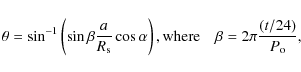
(1)

where t is the time, measured with respect to the transit center, and given in hours, $P_{\rm o}$ is the orbital period in days, and $\alpha$ is the latitude of the transit. The above equation is used to estimate the initial spot longitude, which was one of the parameters to be determined from the model fit to the data.

The next step was to decide the maximum number of spots that were needed to fit each transit. Models with a maximum of 7, 8, and 9 spots on the stellar surface during each transit were tried. The results obtained from each run were qualitatively similar in all cases. It was found that in the case of 9 spots, the residuals were smaller than the uncertainty of the data (0.0006). Therefore, the results reported here are those from the fits for up to a total of nine different spots per transit.

4 The physical parameters of spots

CoRoT-2 is a very active star, and many intensity variations were identified in each transit (see Fig. 1), implying that there are many spots present on the surface of the star at any given time. Beside its longitude, the spot signature also depends on its intensity and size: the flux perturbation caused by the spot is indeed the product of the spot intensity and its area. Thus there is a degeneracy between the values of the radius and intensity determined for a given spot. However, the shape of the signal depends on the radius of the spot. Smaller spots display a slightly narrower feature with a more triangular shape.

Despite allowing the longitude to be a free parameter (determined from the fit), the spot latitude remained constant at $-14.6^\circ$ (the transit latitude). The longitude considered here is the topocentric longitude, that is, the zero angle is defined to be that of the line-of-sight, or transit center, when star, planet, and Earth are aligned.

The light curve was modeled by a star with 9 spots, each with three free parameters (radius, intensity, and longitude) that were obtained from the fit. An example of the fitting is shown in Fig. 4 for the 7th transit. The top panel represents the synthesized star with spots of varying intensity (with respect to $I_{\rm c}$ ) and radius (in units of $R_{\rm p}$ ). The residuals of the data minus the fit are shown in the bottom panel of the figure, and is basically less than the data noise of 0.0006 throughout the transit (within the two vertical dotted lines).

$\begin{figure} \par\includegraphics[width=8cm,clip]{11904fg4.eps} \end{figure}$	Figure 4: Top: example of the model synthesized star with 9 spots for transit 7. Bottom: residuals of the fit minus the data.
Open with DEXTER

The spot contrast is taken to be $1-f_{\rm i}$ , where $f_{\rm i}$ is the relative intensity of the spot with respect to the disk center intensity, $I_{\rm c}$ . A quantity that can be estimated is the total flux subtracted from the star by the presence of spots. This relative flux deficit for a single spot is the product of the spot contrast and its area, that is, $F \propto (1-f_{\rm i}) R_{\rm spot}^2$ . For each transit, the total flux deficit associated with spots was calculated by summing the flux of all individual spots. Figure 5 shows the total relative flux calculation for each transit.

$\begin{figure} \par\includegraphics[width=9cm,clip]{11904fg5.eps} \end{figure}$	Figure 5: Temporal evolution of the total relative flux deficit from all spots per transit.
Open with DEXTER

However, not all spots obtained by the fit produce a significant signal in the light curve. By significant, we mean that the maximum relative flux deficit caused by the spot is above the data noise of 0.0006. From the analysis of the results from simulations of single spots with varying radius and intensity, it was found that a signal in the light curve was higher than 0.0006 only when the spot flux was above 0.02 (dotted line of Fig. 5). Therefore, only those spots with flux above the threshold of 0.02 are considered in the results presented below.

4.1 Spot longitudes

A histogram of the spot longitudes is shown in the top panel of Fig. 6. These are topocentric longitudes, that is, they are not the ones located on the rotating frame of the star, but rather are measured with respect to an external reference frame. To obtain the longitudes in the stellar rotating frame, one needs an accurate period for the star. Alonso et al. (2008) report a 4.54 days period, whereas Lanza et al. (2009) obtain a period of $4.52 \pm 0.14$ days when fitting the rotational modulation of the out-of-transit data. A more precise estimate of the period is needed before analyzing the spot results. A detailed investigation of the rotational longitudes and the spot lifetime is underway and will be reported in an accompanying paper (Silva-Valio & Lanza 2010, A&A, in prep.).

$\begin{figure} \par\includegraphics[width=9cm,clip]{11904fg6.eps} \end{figure}$	Figure 6: Histograms with the spot parameters obtained from the fits to the light curve transits: a) longitude, b) radius in units of $R_{\rm p}$ , c) intensity in units of $I_{\rm c}$ , and d) temperature.
Open with DEXTER

4.2 Spot radius

The distribution of spot radius obtained from the fits to all transit data is shown in Fig. 6b. The results show that the radius of the modeled spots varies from 0.2 to 0.7 $R_{\rm p}$ , with a mean value of $0.46 \pm 0.11\ R_{\rm p}$ . Assuming a planet of $1.465\ R_{\rm Jup}$ , these size estimates are equivalent to spots with diameters of 40 to 150 Mm, with a mean value of about 100 Mm.

4.3 Spot intensity and temperature

Spots with lower intensity values, or higher contrast spots, are spots cooler than those with intensity values close to $I_{\rm c}$ . The spot intensities obtained from the model are shown in Fig. 6c. The figure shows that the spot intensities range from 0.3 to 0.8 $I_{\rm c}$ with an average value of $0.55 \pm 0.13$ of the stellar central intensity. The value of $0.665~I_{\rm c}$ used by Lanza et al. (2009), which is the mean value of spots on the Sun, is within the mean spot intensity of CoRoT-2 and its uncertainty.

These intensities can be converted to spot temperature by assuming blackbody emission for both the photosphere and the spots. The temperature is estimated to be

$\begin{displaymath}T_{\rm spot} = {{h \nu} \over K_{\rm B}} \left[ \ln \left( 1 ... ...m eff}}}\right)} - 1} \over f_{\rm i}} \right) \right]^{-1}\!, \end{displaymath}$

(2)

where $K_{\rm B}$ and h are the Boltzmann and Planck constants, respectively, $\nu$ is the frequency associated with a wavelength of 600 nm, $f_{\rm i}$ is the fraction of spot intensity with respect to the central stellar intensity $I_{\rm c}$ , and $T_{\rm eff}$ is the effective temperature of the star. Considering $T_{\rm eff}=5625$ K (Alonso et al. 2008), the spot temperatures range from 4000 to 5300 K, which are 300-1600 K cooler than the remainder of the disk. The mean temperature of spots on CoRoT-2 is $4700 \pm 300$ K, about 1000 K cooler than the photosphere.

4.4 Stellar surface area covered by spots

By considering only the spots with fluxes above 0.02, the number of spots on the surface of the star during each transit varied from 2 to 9 spots, with an average number of $8 \pm 1$ . The transit with the smallest number of spots (2) corresponds to the 32nd transit discussed before. A histogram of the number of spots per transit is shown in the top panel of Fig. 7.

$\begin{figure} \par\includegraphics[width=9cm,clip]{11904fg7.eps} \end{figure}$	Figure 7: Top: distribution of the number of spots detected on each planetary transit. Middle: histogram of the stellar surface area covered by spots within the transit latitudes. Bottom: temporal evolution of the stellar surface area covered by spots in each transit.
Open with DEXTER

The mean surface area covered by the spots during each transit is the sum of the area of all spots detected in that transit divided by the total area occulted by the passage of the planet (see the diagram in Fig. 8). The total area, $A_{\rm tot}$ , of the transit band occulted by the planet is calculated to be

$\displaystyle A_{\rm tot} = 2 R_{\rm p} {7 \over 9} \pi \ {(x_1 + x_2) \over 2} R_{\rm s},$

(3)

$\displaystyle {\rm where} \quad x_1$	=	$\displaystyle \sqrt{1-\left[ \sin\alpha - {R_{\rm p} \over R_{\rm s}}\right]^2} ,$	(4)
x₂	=	$\displaystyle \sqrt{ 1-\left[ \sin\alpha + {R_{\rm p} \over R_{\rm s}}\right]^2 \cdot}$	(5)

The 7/9 factor arises because in this fit, only spots between longitudes $-70^\circ$ and $+70^\circ$ are considered because of the difficulties in fitting spots too close to the limb, where the light curve is very steep.

$\begin{figure} \par\includegraphics[width=6cm,clip]{11904fg8.eps} \vspace*{2mm} \end{figure}$	Figure 8: Diagram of the total area of the star occulted by the planet transit, represented by the hatched region.
Open with DEXTER

The star surface area covered by spots is the sum of the area of all spots, that is, $\Sigma\ \pi R_{\rm spot}^2$ , where $R_{\rm spot}$ is the radius of the spot obtained from the fits. The surface area covered by spots on each transit, taking into account only the area of the transit band, of course, computed from the above equation is shown in the bottom panels of Fig. 7 as a histogram, and the temporal evolution. The average value of the stellar surface area covered by spots is $16 \pm 5$ %, shown as a dashed line in the bottom panel of Fig. 7.

5 Discussion and conclusions

CoRoT-2 star is a young and reasonably active star. Spots on the surface of the star can influence the determination of the orbital parameters of a planet by distorting the transit light curve in two ways (Silva-Valio 2010). One is the presence of spots on the limb of the star which will cause the transit duration to be shorter than it really is. The other distortion involves making the transit shallower if there are many spots on the surface of the star. This would cause the planet radius estimate to be smaller than its real value. The latter effect was observed in the dataset analyzed here, where the spot model applied yielded a radius of 0.172 $R_{\rm star}$ instead of the 0.1667 $R_{\rm star}$ listed in Alonso et al. (2008). In this case, we do not believe that this represents a real difference in the planet radius, but rather an artifact of the spot distribution on the surface of the star at any given time.

Here the star was modeled as having up to 9 round spots at any given time on its surface at certain positions (latitude and longitude) during the uninterrupted 134 days of observation by the CoRoT satellite. For each transit, the longitudes of the spots were obtained from a fit of the model to the data. Also obtained from the fit, the other free parameters were the spot radius and its intensity. On every transit, there were, on average, 7 to 9 spots on the visible stellar hemisphere within longitudes of $\pm 70^\circ$ , considering only spots with flux above 0.02.

The spot radius ranged from 0.2 to 0.7 $R_{\rm p}$ , with a mean value of $0.46 \pm 0.11\ R_{\rm p}$ , whereas the intensity was between 0.3 and 0.8 $I_{\rm c}$ with an average of $0.55 \pm 0.13\ I_{\rm c}$ . This mean intensity is close to the value of $0.665~I_{\rm c}$ used by Lanza et al. (2009), which is the same as the sunspot bolometric contrast (Chapman et al. 1994). From these intensities, the mean temperature of the spots was estimated to be $4700 \pm 300$ K by considering black-body emission for both the stellar photosphere and spots. These spots are about 1000 K cooler than the surrounding photosphere ( $T_{\rm eff}=5625$ ).

Wolter et al. (2009) modeled a single spot on one transit (here transit 54 of Fig. 1). The authors modeled the spot with different intensities, analogous to our procedure, and obtained a spot radius of $4.8^\circ$ (in degrees of stellar surface) for $0.3\ I_{\rm c}$ . This specific feature, a ``bump" on the light curve transit wasreproduced more successfully by our model with two spots at longitudes of 2 and 15 $^\circ$ , of radius of 0.49 and $0.54~R_{\rm p}$ and spot intensity of 0.6 $I_{\rm c}$ for both spots (half the contrast of the single Wolter 2009, spot). These radii are equivalent to 4.9 and $5.4^\circ$ , very similar to the results obtained by Wolter et al. (2009) which also confirm the spot degeneracy between size and contrast. Spots of smaller contrast (higher intensity relative to the photosphere) need to be larger to account for the detected flux deficit.

The spots on CoRoT-2, with diameters of the order of $\sim$ 100 000 km, are much larger than sunspots, being about 10 times the size of a large sunspot (10 Mm). The mean surface area of the star covered by spots within the transit latitudes is in the range 10-20%. This is larger than the 7 to 9% of the total spotted area found by Lanza et al. (2009). However, these values were estimated by considering the whole star, that is, also the pole areas, where there are no spots in the case of the Sun. The values obtained here only are for the transit latitudes, which span approximately $20^\circ$ and are close to the equator. In this case, the latitudes coincide with the so-called royal latitudes of the Sun, where the majority of sunspots occurs.

Long-term observations such as the one provided by CoRoT are paramount to understanding the physics of star spots. The model applied here to the CoRoT-2 data is capable of determining the physical properties of spots with the advantage of following their temporal evolution, as will be described in an accompanying paper (Silva-Valio & Lanza 2010, A&A, in prep.). It will be very interesting to perform similar analyzes on data from other stars with planetary transits observed by the CoRoT satellite, especially for stars that are not solar-like.

Acknowledgements

We would like to thank the referee, G. A. Wade, for useful suggestions that helped improve the paper. Also, the authors are grateful to everyone involved in the planning and operation of the CoRoT satellite which made these observations possible. A.S.V. acknowledges partial financial support from the Brazilian agency FAPESP (grant number 2006/50654-3).

Note added in proof. It is reassuring to see that analyses of the same data by Czesla et al. (A&A, 2009, 505, 1277) and Huber et al. (A&A, 2009, 508, 901) corroborate the results presented here.

References

Alonso, R., Auvergne, A., Baglin, A., et al. 2008, A&A, 482, L21 [NASA ADS] [CrossRef] [EDP Sciences] [Google Scholar]
Baglin, A., Auvergne, M., Boirnard, L., et al. 2006, 36th COSPAR Scientific Assembly, 36, 3749 [Google Scholar]
Blanter, E. M., Mouël, J.-L., Le, Perrier, F., & Shnirman, M. G. 2006, Sol. Phys., 237, 329 [NASA ADS] [CrossRef] [Google Scholar]
Bouchy, F., Queloz, D., Deleuil, M., et al. 2008, A&A, 482, L25 [NASA ADS] [CrossRef] [EDP Sciences] [Google Scholar]
Chapman, G. A., Cookson, A. M., & Dobias, J. J. 1994, ApJ, 432, 403 [NASA ADS] [CrossRef] [Google Scholar]
Hathaway, D. H., & Choudhary, D. P. 2008, Sol. Phys., 250, 269 [NASA ADS] [CrossRef] [Google Scholar]
Lanza, A. F., Pagano, I., Leto, G., et al. 2009, A&A, 493, 193 [NASA ADS] [CrossRef] [EDP Sciences] [Google Scholar]
Petrovay, K., & van Driel-Gesztelyi, L. 1997, Sol. Phys., 176, 249 [NASA ADS] [CrossRef] [Google Scholar]
Pont, F., Gilliland, R. L., Moutou, C., et al. 2007, A&A, 476, 1347 [NASA ADS] [CrossRef] [EDP Sciences] [MathSciNet] [Google Scholar]
Press, W. J., Teukolsky, S. A., Vetterling, W. T., & Flannery, B. P. 1992, Numerical recipes in FORTRAN, The art of scientific computing, 2nd edition (Cambridge: University Press) [Google Scholar]
Silva, A. V. R. 2003, ApJ, 585, L147 [NASA ADS] [CrossRef] [Google Scholar]
Silva-Valio, A. 2008, ApJ, 683, L179 [NASA ADS] [CrossRef] [Google Scholar]
Silva-Valio, A. 2010, in Solar and Stellar Variability Impact on Earth and Planets, 3-7 August 2009, Rio de Janeiro, Brazil, Proc. IAU Symp., 264, in press [Google Scholar]
Wolter, U., Schmitt, J. H. M. M., Huber, K. F., et al. 2009, A&A, 504, 561 [NASA ADS] [CrossRef] [EDP Sciences] [Google Scholar]

Footnotes

... CoRoT-2: CoRoT is a space project operated by the French Space Agency, CNES, with participation of the Science Programme of ESA, ESTEC/RSSD, Austria, Belgium, Brazil, Germany, and Spain.

All Figures

$\begin{figure} \par\includegraphics[width=9cm,clip]{11904fg1.eps} \vspace{4mm} \end{figure}$	Figure 1: All the 77 light curves during the transit of CoRoT-2b in front of its spotted host star. The gray solid line represent the model of a spotless star. The error bars of the data points indicate the rms of 0.0006.
Open with DEXTER
In the text

$\begin{figure} \par\includegraphics[width=9cm,clip]{11904fg2.eps} \vspace*{-2mm} \end{figure}$	Figure 2: Top: examples of transit light curves of CoRoT-2. The black crosses represent the 32nd transit assumed to occur when the star has minimum spot activity within the transit latitudes, whereas the gray (red crosses in the color version) data points represent a typical transit (the fifth one). The model light curve without any spots is shown as the thick solid curve. Bottom: residual from the subtraction of the data minus the model for a star with no spots for the 5th (gray/red) and 32nd (black) transits. The vertical bars in both panels represent the estimated uncertainty of 0.0006 from out of transit data.
Open with DEXTER
In the text

$\begin{figure} \par\includegraphics[width=8cm]{11904fg3.eps} \end{figure}$	Figure 3: Top: top view of the star and the planet in its orbit. A spot at 45 $^\circ$ longitude on the stellar surface is depicted. Bottom: light curve obtained from a star with a spot at 45 $^\circ$ longitude. The dotted line represents a model for a transit in front of a spotless star.
Open with DEXTER
In the text

$\begin{figure} \par\includegraphics[width=8cm,clip]{11904fg4.eps} \end{figure}$	Figure 4: Top: example of the model synthesized star with 9 spots for transit 7. Bottom: residuals of the fit minus the data.
Open with DEXTER
In the text

$\begin{figure} \par\includegraphics[width=9cm,clip]{11904fg5.eps} \end{figure}$	Figure 5: Temporal evolution of the total relative flux deficit from all spots per transit.
Open with DEXTER
In the text

$\begin{figure} \par\includegraphics[width=9cm,clip]{11904fg6.eps} \end{figure}$	Figure 6: Histograms with the spot parameters obtained from the fits to the light curve transits: a) longitude, b) radius in units of $R_{\rm p}$ , c) intensity in units of $I_{\rm c}$ , and d) temperature.
Open with DEXTER
In the text

$\begin{figure} \par\includegraphics[width=9cm,clip]{11904fg7.eps} \end{figure}$	Figure 7: Top: distribution of the number of spots detected on each planetary transit. Middle: histogram of the stellar surface area covered by spots within the transit latitudes. Bottom: temporal evolution of the stellar surface area covered by spots in each transit.
Open with DEXTER
In the text

$\begin{figure} \par\includegraphics[width=6cm,clip]{11904fg8.eps} \vspace*{2mm} \end{figure}$	Figure 8: Diagram of the total area of the star occulted by the planet transit, represented by the hatched region.
Open with DEXTER
In the text

Current usage metrics show cumulative count of Article Views (full-text article views including HTML views, PDF and ePub downloads, according to the available data) and Abstracts Views on Vision4Press platform.

Data correspond to usage on the plateform after 2015. The current usage metrics is available 48-96 hours after online publication and is updated daily on week days.

Initial download of the metrics may take a while.

[1] Alonso, R., Auvergne, A., Baglin, A., et al. 2008, A&A, 482, L21 [NASA ADS] [CrossRef] [EDP Sciences] [Google Scholar]

[2] Baglin, A., Auvergne, M., Boirnard, L., et al. 2006, 36th COSPAR Scientific Assembly, 36, 3749 [Google Scholar]

[3] Blanter, E. M., Mouël, J.-L., Le, Perrier, F., & Shnirman, M. G. 2006, Sol. Phys., 237, 329 [NASA ADS] [CrossRef] [Google Scholar]

[4] Bouchy, F., Queloz, D., Deleuil, M., et al. 2008, A&A, 482, L25 [NASA ADS] [CrossRef] [EDP Sciences] [Google Scholar]

[5] Chapman, G. A., Cookson, A. M., & Dobias, J. J. 1994, ApJ, 432, 403 [NASA ADS] [CrossRef] [Google Scholar]

[6] Hathaway, D. H., & Choudhary, D. P. 2008, Sol. Phys., 250, 269 [NASA ADS] [CrossRef] [Google Scholar]

[7] Lanza, A. F., Pagano, I., Leto, G., et al. 2009, A&A, 493, 193 [NASA ADS] [CrossRef] [EDP Sciences] [Google Scholar]

[8] Petrovay, K., & van Driel-Gesztelyi, L. 1997, Sol. Phys., 176, 249 [NASA ADS] [CrossRef] [Google Scholar]

[9] Pont, F., Gilliland, R. L., Moutou, C., et al. 2007, A&A, 476, 1347 [NASA ADS] [CrossRef] [EDP Sciences] [MathSciNet] [Google Scholar]

[10] Press, W. J., Teukolsky, S. A., Vetterling, W. T., & Flannery, B. P. 1992, Numerical recipes in FORTRAN, The art of scientific computing, 2nd edition (Cambridge: University Press) [Google Scholar]

[11] Silva, A. V. R. 2003, ApJ, 585, L147 [NASA ADS] [CrossRef] [Google Scholar]

[12] Silva-Valio, A. 2008, ApJ, 683, L179 [NASA ADS] [CrossRef] [Google Scholar]

[13] Silva-Valio, A. 2010, in Solar and Stellar Variability Impact on Earth and Planets, 3-7 August 2009, Rio de Janeiro, Brazil, Proc. IAU Symp., 264, in press [Google Scholar]

[14] Wolter, U., Schmitt, J. H. M. M., Huber, K. F., et al. 2009, A&A, 504, 561 [NASA ADS] [CrossRef] [EDP Sciences] [Google Scholar]