| Issue |
A&A
Volume 510, February 2010
|
|
|---|---|---|
| Article Number | A106 | |
| Number of page(s) | 9 | |
| Section | Stellar structure and evolution | |
| DOI | https://doi.org/10.1051/0004-6361/200811438 | |
| Published online | 18 February 2010 | |
The nature of p-modes and granulation in HD 49933 observed by CoRoT![[*]](/icons/foot_motif.png)
T. Kallinger1,2 - M. Gruberbauer1,3 - D. B. Guenther3 - L. Fossati1 - W. W. Weiss1
1 - Institute for Astronomy (IfA), University of Vienna, Türkenschanzstrasse 17, 1180 Vienna, Austria
2 -
Department of Physics and Astronomy, University of British Columbia, 6224 Agricultural Road, Vancouver, BC V6T 1Z1, Canada
3 - Institute for Computational Astrophysics, Department of
Astronomy and Physics, Saint Marys University, Halifax, NS B3H 3C3,
Canada
Received 28 November 2008 / Accepted 20 November 2009
Abstract
Context. Recent observations of HD 49933 by the space-photometric mission CoRoT provide photometric
evidence of solar type oscillations in a star other than our Sun. The
first published reduction, analysis, and interpretation of the CoRoT
data yielded a spectrum of p-modes with l = 0, 1, and 2.
Aims. We present our own analysis of the CoRoT data in an
attempt to compare the detected pulsation modes with eigenfrequencies
of models that are consistent with the observed luminosity and surface
temperature.
Methods. We used the Gruberbauer et al. frequency set
derived based on a more conservative Bayesian analysis with ignorance
priors and fit models from a dense grid of model spectra. We also
introduce a Bayesian approach to searching and quantifying the best
model fits to the observed oscillation spectra.
Results. We identify 26 frequencies as radial and dipolar modes.
Our best fitting model has solar composition and coincides within the
error box with the spectroscopically determined position of
HD 49933 in the H-R diagram. We also show that lower-than-solar Z
models have a lower probability of matching the observations than the
solar metallicity models. To quantify the effect of the deficiencies in
modeling the stellar surface layers in our analysis, we compare
adiabatic and nonadiabatic model fits and find that the latter
reproduces the observed frequencies better.
Key words: stars: late-type - stars: oscillations - stars: fundamental parameters - stars: individual: HD 49933 - techniques: photometric
1 Introduction
CoRoT (Convection, Rotation, and planetary Transits) is a space
mission focusing on asteroseismology and the detection of exoplanetary
transits. See Boisnard & Auvergne (2006) for an overview of the technical details and Baglin et al. (2006) for a review of the asteroseismology aspects of the mission.
HD 49933 (F5 V, mV=5.77) is a main sequence star with an effective temperature of about 6500 K,
![]()
![]() ,
,
![]() ,
and
,
and
![]() .
The determination of these values is described in our Sect. 2.
HD 49933 is similar to Procyon, except with a lower metal
abundance. HD 49933 was observed during the initial run of CoRoT
from February 6 to April 7, 2007, only little more than one month after
launch of CoRoT on December 27, 2006.
.
The determination of these values is described in our Sect. 2.
HD 49933 is similar to Procyon, except with a lower metal
abundance. HD 49933 was observed during the initial run of CoRoT
from February 6 to April 7, 2007, only little more than one month after
launch of CoRoT on December 27, 2006.
The reduction of the CoRoT photometry to the N2 data format is described in Appourchaux et al. (2008). They also provide the first frequency determination, a preliminary echelle diagram, and a mode identification for HD 49933. Because their conclusions differ from ours we review their procedure here highlighting areas where we have adopted a different set of premises. They use a maximum likelihood estimator technique to fit Lorentzian mode profiles to the observed power spectrum with symmetric rotational splitting components included with the non-radial modes. In order to reduce the number of free parameters, they assume the same line width for modes of the same radial order, and they assume the mode heights are related to each other by fixed ratios. For the rotational splitting components, they assume the splitting is symmetric in frequency with the split-mode height ratios determined from the inclination angle parameter.
Our approach to identifying frequencies (Gruberbauer et al. 2009, hereafter Paper I) is distinct, in that we emphasize the reliability of the frequency detections over the quantity of detected frequencies. Without prejudging the identity of a mode, we first simply ask if a mode is statistically visible in the data. Then when we have ascertained its existence above some statistical measure, we try to fit stellar models to the resultant list of frequencies. When comparing observed frequencies with stellar model frequencies, even a few incorrectly identified frequencies can significantly complicate the analysis or even lead to a misinterpretation.
In Paper I we describe the fitting of solar-type p-modes as a parameter estimation problem without the need to give preference to any specific model. A Markov-Chain, Monte Carlo technique for a Bayesian analysis of Lorentzian profiles was used rather than fitting complex models to the observations. Specifically, we did not make any assumptions about mode heights, knowing that noise in the data, itself, can affect the observed heights of individual modes. Rather, we used our fits to the mode heights compared to the noise level to characterize the viability of the mode being detected. We, therefore, only assumed the Lorentzian profiles have the same line width. This assumption might distort the correct determination of the mode height and line width parameters, because it is known, e.g., for the Sun (e.g. Chaplin et al. 2005), that the mode lifetime is a function of frequency. To fix the mode line widths to a single parameter, however, should not (or only marginally) influence the determination of the mode frequencies, which is the parameter we are most interested in. We extracted a number of radial and l = 1 modes. We found no evidence in the CoRoT data of statistically signifiant l = 2 modes or for rotationally split components. If they exist, of course, these components are below the threshold of our mode-height-detection criterion. We argue that the Appourchaux et al. (2008) approach is too restrictive in that it presumes specific characteristics of the modes identity. At this early stage in the analysis of such stars, we are not comfortable making any assumptions about the modes even at the expense of identifying fewer modes.
In Sect. 2 we re-examine the fundamental parameter determinations of HD 49933. In Sect. 3 we describe two methods for searching large grids of stellar models for a best fit between observed and model frequencies. One of the methods, again a Bayesian approach, allows us to estimate the statistical likelihood of the fit compared to other models in our grids. Our best fitting model has solar composition and is located in the H-R diagram within the spectroscopically determined error box of HD 49933.
2 Fundamental parameters
Eight different values for the effective temperature, based on spectroscopy and photometry and ranging from 6467 K to 6780 K are cited by Gillon & Magain (2006). Blackwell & Lynas-Gray (1998) determined the effective temperature to be 6512 K by using the IR flux method. In their paper on the CoRoT asteroseismic observations of HD 49933, Appourchaux et al. (2008) adopt an effective temperature of 6780In February 2006, 10 high-resolution spectra (
![]() )
were obtained for HD 49933 with the HARPS spectrograph at the
ESO-LaSilla 3.6 m telescope. We retrieved these spectra from the
ESO archive and increased the signal-to-noise ratio (
)
were obtained for HD 49933 with the HARPS spectrograph at the
ESO-LaSilla 3.6 m telescope. We retrieved these spectra from the
ESO archive and increased the signal-to-noise ratio (![]() 500
in a 0.5 Å continuum bin around 5000 Å) by co-adding. The
continuum normalization was done with a low order polynomial fit to
regions free of visible spectral lines.
500
in a 0.5 Å continuum bin around 5000 Å) by co-adding. The
continuum normalization was done with a low order polynomial fit to
regions free of visible spectral lines.
![\begin{figure}
\par\includegraphics[width=9cm,clip]{11438fig1.eps} \vspace*{5mm}
\end{figure}](/articles/aa/full_html/2010/02/aa11438-08/img16.png)
|
Figure 1:
Observed H |
| Open with DEXTER | |
To derive a consistent and reliable value for
![]() we compared the observed hydrogen line profiles with synthetic spectra computed with S YNTH3 (Kochukhov 2007). In the given temperature range the hydrogen lines are very sensitive to temperature variations, are less sensitive to
we compared the observed hydrogen line profiles with synthetic spectra computed with S YNTH3 (Kochukhov 2007). In the given temperature range the hydrogen lines are very sensitive to temperature variations, are less sensitive to
![]() variations, and depend on the metallicity of the atmosphere. We calculated model atmospheres with LL MODELS (Shulyak et al. 2004),
an LTE code that uses direct sampling of the line opacities and allows
models to be computed with an individualized abundance pattern. Mg I line wings (
variations, and depend on the metallicity of the atmosphere. We calculated model atmospheres with LL MODELS (Shulyak et al. 2004),
an LTE code that uses direct sampling of the line opacities and allows
models to be computed with an individualized abundance pattern. Mg I line wings (
![]() 5167 5172, 5183 Å; Fuhrmann et al. 1997)
and the ionization equilibrium of several additional elements were used
to determine the gravity. We started our model atmosphere iteration
with the most convincing value of
5167 5172, 5183 Å; Fuhrmann et al. 1997)
and the ionization equilibrium of several additional elements were used
to determine the gravity. We started our model atmosphere iteration
with the most convincing value of
![]() ,
based on models with solar abundances, and a surface gravity derived
from photometry. We derived the abundances of several elements from
equivalent widths and then determined
,
based on models with solar abundances, and a surface gravity derived
from photometry. We derived the abundances of several elements from
equivalent widths and then determined
![]() from a set of models using the previously obtained
from a set of models using the previously obtained
![]() and abundances. With this value for the gravity we determined anew the abundances and used them to improve
and abundances. With this value for the gravity we determined anew the abundances and used them to improve
![]() .
After two iterations we converged to
.
After two iterations we converged to
![]() K and
K and
![]() ,
which is significantly cooler than the value adopted by Appourchaux et al. (2008). The small error in
,
which is significantly cooler than the value adopted by Appourchaux et al. (2008). The small error in
![]() can be explained by the high temperature sensitivity of the hydrogen line profiles (see left panel of Fig. 1). Regardless, for the following considerations we adopt a more conservative error for the effective temperature of
can be explained by the high temperature sensitivity of the hydrogen line profiles (see left panel of Fig. 1). Regardless, for the following considerations we adopt a more conservative error for the effective temperature of ![]() 75 K.
The atomic line parameters were taken from the VALD database (Piskunov et al. 1995; Ryabchikova et al. 1999; Kupka et al. 1999), except for the Van der Waals broadening constants, which were taken from Fuhrmann et al. (1997). The quoted error for
75 K.
The atomic line parameters were taken from the VALD database (Piskunov et al. 1995; Ryabchikova et al. 1999; Kupka et al. 1999), except for the Van der Waals broadening constants, which were taken from Fuhrmann et al. (1997). The quoted error for
![]() is similar to other stars with comparable effective temperatures, such as Procyon (Fuhrmann et al. 1997), and using the same method.
is similar to other stars with comparable effective temperatures, such as Procyon (Fuhrmann et al. 1997), and using the same method.
It is useful in asteroseismic modeling to know the metallicity of the
star. According to our spectroscopic analysis the atmospheric
metallicity is
![]() where iron is under abundant compared to the Sun (Grevesse et al. 1996),
in agreement with published values. Carbon and oxygen, on the other
hand, have near solar abundances. This variation could be due to the
effects of gravitational settling and radiative levitation in the thin
convective envelope of the star. The true interior abundance, relevant
for stellar models and pulsation analysis, is uncertain. Ideally,
stellar models should include the effects of element diffusion. Further
details of the spectroscopic analysis with a discussion of the
literature can be found in Ryabchikova et al. (2009).
where iron is under abundant compared to the Sun (Grevesse et al. 1996),
in agreement with published values. Carbon and oxygen, on the other
hand, have near solar abundances. This variation could be due to the
effects of gravitational settling and radiative levitation in the thin
convective envelope of the star. The true interior abundance, relevant
for stellar models and pulsation analysis, is uncertain. Ideally,
stellar models should include the effects of element diffusion. Further
details of the spectroscopic analysis with a discussion of the
literature can be found in Ryabchikova et al. (2009).
Using the Hipparcos parallax
![]() mas (van Leeuwen 2007) we abtain the absolute visual magnitude
mas (van Leeuwen 2007) we abtain the absolute visual magnitude
![]() .
Interpolating the tables of Lejeune & Schaerer (2001) we obtain a bolometric correction BC
.
Interpolating the tables of Lejeune & Schaerer (2001) we obtain a bolometric correction BC
![]() (for
(for
![]() ), which is more than twice the value used by Appourchaux et al. (2008). With
), which is more than twice the value used by Appourchaux et al. (2008). With
![]() we obtain
we obtain
![]() (Appourchaux et al. 2008, use
(Appourchaux et al. 2008, use
![]() )
and a corresponding radius of
)
and a corresponding radius of
![]() .
.
3 Asteroseismic analysis
For our analysis we use the frequencies given in Paper I (see Table 5 therein) where we exclude P25 and P26 following the suggestion of the authors. They did not assign credibility to these values arguing with the ambiguity in their marginal frequency distribution, which is apparent in the listed large uncertainties. In Paper I, no specific mode identifications to the frequencies were assumed and mode heights were left unconstrained. Appourchaux et al. (2008), on the other hand, assumed specific mode identifications (l = 0, 1, and 2) and fixed relative mode heights.We search a dense and extensive grid of stellar model oscillation
spectra looking for the model spectra that matches best the observed
frequencies to within the known uncertainties of the observed
frequencies. We use a simple ![]() formula to quantify how well the spectra match each other. This
approach is fast and efficient and can handle sparse and contaminated
oscillation spectra. Although a lower
formula to quantify how well the spectra match each other. This
approach is fast and efficient and can handle sparse and contaminated
oscillation spectra. Although a lower ![]() does indicate a higher likelihood, the computed
does indicate a higher likelihood, the computed ![]() s
cannot be used to associate a confidence level to the inferred
parameters. We, therefore, introduce a new method based on a Bayesian
approach that uses the error distributions of the observed frequencies
to quantify in terms of a probability how well the frequencies of a
given model match the observations.
s
cannot be used to associate a confidence level to the inferred
parameters. We, therefore, introduce a new method based on a Bayesian
approach that uses the error distributions of the observed frequencies
to quantify in terms of a probability how well the frequencies of a
given model match the observations.
The grids of models were constructed using the Yale Stellar Evolution Code (YREC; Guenther et al. 1992). The grids include models with masses ranging from 0.6 to 2.00
![]() in steps of 0.005
in steps of 0.005
![]() and from 2.00 to 5.00
and from 2.00 to 5.00
![]() in steps of 0.01
in steps of 0.01
![]() .
Each evolutionary track runs from the zero age main sequence to halfway
up the giant branch. The solar grid is based on a near solar
composition and calibrated mixing length parameter (Z = 0.02, Y = 0.27,
.
Each evolutionary track runs from the zero age main sequence to halfway
up the giant branch. The solar grid is based on a near solar
composition and calibrated mixing length parameter (Z = 0.02, Y = 0.27,
![]() ). The low Z
grid, which has the same mass resolution but is not nearly as extensive
in its coverage, is based on the same mixing length parameter and (
Z, Y) = (0.008, 0.24).
). The low Z
grid, which has the same mass resolution but is not nearly as extensive
in its coverage, is based on the same mixing length parameter and (
Z, Y) = (0.008, 0.24).
Table 1: Summary of the best fitting solar-abundance and metal-poor adiabatic and nonadiabatic models for the frequencies given by A: Gruberbauer et al. (2009) and B: Appourchaux et al. (2008).
The constitutive physics of the models include OPAL98 (Iglesias & Rogers 1996), the Alexander & Ferguson (1994) opacity tables, and the Lawrence Livermore National Laboratory equation of state tables (Rogers et al. 1996; Rogers 1986). The standard Böhm-Vitense (Böhm-Vitense 1958; Vitense 1953) mixing length theory is used to model convection. The mixing length parameter used to describe the temperature gradient in convective regions was adjusted from calibrated solar models and rounded to two significant digits. We have assumed standard solar mixture (Grevesse et al. 1996). Although the effects of helium and heavy element diffusion are included in the model physics, diffusion is automatically turned off shortly after turn-off to avoid known computational problems associated with very thin convection zones. Each model was resolved into approximately 2000 shells, with two-thirds of the shells placed in the envelope and atmosphere. Guenthers nonradial nonadiabatic stellar pulsation program (Guenther 1994) was used to compute the adiabatic and nonadiabatic pulsation spectra of each of the models in the grid. The nonabatic code includes the effects of radiation on the modes but does not include the, probably equally important, effects of convection.
3.1  mode matching
We begin our model analysis using the 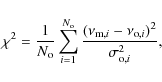
where
To find a best model fit to the 26 observed frequencies (Table 5 in Paper I) we searched for modes from l
= 0 to 3, inclusive. In our range of interest in the H-R diagram the
``resolution'' of our grid, i.e., the step in frequency for a mode of
given degree and radial order from model to model, is about
4 ![]() Hz (
Hz (![]() 0.2%
of the observed frequency with the highest amplitude). This is quite
high compared to the uncertainties in the observations. We therefore
interpolated our grid linearly along the evolutionary tracks,
effectively increasing the grid density by a factor of 10.
0.2%
of the observed frequency with the highest amplitude). This is quite
high compared to the uncertainties in the observations. We therefore
interpolated our grid linearly along the evolutionary tracks,
effectively increasing the grid density by a factor of 10.
The best fitting model using nonadibatic frequencies, in other words, the model with the lowest
![]() ,
matches the observed frequencies with 13 radial and 13 dipole modes. The best fitting model using adiabatic frequencies has
,
matches the observed frequencies with 13 radial and 13 dipole modes. The best fitting model using adiabatic frequencies has
![]() .
The nonadiabatic frequencies provide a better fit than the adiabatic
frequencies. The model itself, though, is only slightly different. We
list the model fit properties in Table 1.
In the top panel of Fig. 2
we provide a direct comparison between the observed frequencies and the
p-mode frequencies of the best fitting model. The echelle diagram shows
that both the adiabatic and nonadibatic model reproduce not only the
general pattern of the observed frequencies, but also the detailed
structure of the mode sequences.
.
The nonadiabatic frequencies provide a better fit than the adiabatic
frequencies. The model itself, though, is only slightly different. We
list the model fit properties in Table 1.
In the top panel of Fig. 2
we provide a direct comparison between the observed frequencies and the
p-mode frequencies of the best fitting model. The echelle diagram shows
that both the adiabatic and nonadibatic model reproduce not only the
general pattern of the observed frequencies, but also the detailed
structure of the mode sequences.
![\begin{figure}
\par\includegraphics[width=8.6cm,clip]{11438fig2.eps}\vspace*{1.5mm}
\includegraphics[width=8.6cm,clip]{11438fig3.eps}
\end{figure}](/articles/aa/full_html/2010/02/aa11438-08/img51.png)
|
Figure 2: Top panel: echelle diagram of the observed oscillation frequencies and the adiabatic and nonadiabatic eigenfrequencies of the best fitting model from the solar abundance model grid. The observed frequencies are shown as filled circles with the error bars indicating the observational uncertainties. The nonadiabatic model frequencies used in the analysis are displayed with gray symbols connected by line segments. The adiabatic frequencies are indicated by line segments only. Bottom panel: same as above, but for the best fitting metal-poor model. |
| Open with DEXTER | |
A theoretical H-R diagram is shown in Fig. 4
representing the subset of the stellar model grid used for the
pulsation analysis, the error box for the effective temperature and
luminosity of HD 49933, and the best nonadiabatic model fits to
the observed frequencies with ![]() less than 4.0. The adiabatic model fits yield a nearly identical plot.
The best fitting nonadiabatic model, located within the error box for
HD 49933, has an effective temperature of
less than 4.0. The adiabatic model fits yield a nearly identical plot.
The best fitting nonadiabatic model, located within the error box for
HD 49933, has an effective temperature of
![]() K, a luminosity of
K, a luminosity of
![]() ,
a radius of
,
a radius of
![]() ,
a mass of
,
a mass of
![]() ,
and an age of 2.15 Gyr (see Table 1).
,
and an age of 2.15 Gyr (see Table 1).
Even though our model searches included l = 0, 1, 2, and 3 p modes, our best adiabatic and nonadiabatic model fits do not need to use any l = 2 and 3 modes and, as a consequence, our mode identifications are different from Appourchaux et al. (2008). This is not an issue of insufficient frequency resolution. If they could be detected in the data, the l = 2 and 3 mode frequencies form a sequence in the echelle diagram separated from the radial mode sequence by a spacing that is several times greater than the frequency uncertainties. Unlike the l = 0 and 2 modes, the l = 0 and 1 are well separated and nearly independent of each other.
If we search our nonadiabatic grid for a best match between the model frequencies given by Appourchaux et al. (2008) and if we use only those identified by them to come from l = 0 and 1 modes we, find no model with a ![]() better than 19.6. This model (
better than 19.6. This model (
![]() , 6487 K) is very close to our best model (see Table 1) and indicates that - on average - the frequency subset derived by Appourchaux et al. (2008) is similar to our frequency set, which is not really surprising as we are using the same data. The high
, 6487 K) is very close to our best model (see Table 1) and indicates that - on average - the frequency subset derived by Appourchaux et al. (2008) is similar to our frequency set, which is not really surprising as we are using the same data. The high ![]() value, however, indicates that their frequency values scatter quite a
bit around those predicted by (our) models and the frequency
uncertainties are underestimated (by up to a factor of 5) in contrast
to our frequencies and uncertainties, derived with a Bayesian approach,
and which result in a
value, however, indicates that their frequency values scatter quite a
bit around those predicted by (our) models and the frequency
uncertainties are underestimated (by up to a factor of 5) in contrast
to our frequencies and uncertainties, derived with a Bayesian approach,
and which result in a
![]() (see Table 1 and Fig. 3). But more importantly, the mode identifications in our analysis are different from that is advocated by Appourchaux et al. (2008). If we force our search program to use their frequencies and l-value identification, we obtain a
(see Table 1 and Fig. 3). But more importantly, the mode identifications in our analysis are different from that is advocated by Appourchaux et al. (2008). If we force our search program to use their frequencies and l-value identification, we obtain a
![]() and a model temperature difference of more than 1000 K.
and a model temperature difference of more than 1000 K.
The mass and age of our best model fit depends on the assumed composition of the model grid. We choose primarily for reference purposes a solar composition grid with ( Y, Z) = (0.27, 0.02). As discussed in Sect. 2, our model atmospheres indicate that HD 49933 is metal poor compared to the Sun, but with solar C and O abundances! Therefore, a more realistic composition for HD 49933 would be closer to ( Y, Z) = (0.24, 0.008) assuming normal rates of the Galactic enrichment of helium and metals. Because we do not have a full grid for this specific composition available, we computed a smaller grid of about 10 000 models centered on the previously best fitting model.
Repeating the analysis with the lower Z adabatic and nonadiabatic grids, we obtained the echelle diagram for the best fitting model, which is presented in the bottom panel of Fig. 2. Apparently, the low-Z fit is not as good as the solar-Z fit. One must be careful, though, not to conclude that HD 49933 has a solar Z, since we do not know the intrinsic model uncertainties exactly. For our Sun, for example, we know that the frequencies of our best solar models differ by up to 0.5% from the observed frequencies for higher radial orders, i.e., higher frequencies. This discrepancy is attributed to known deficiencies in the modeling of the surface layers.
With frequency uncertainties in asteroseismic observations approaching ![]() 0.5
0.5 ![]() Hz,
it is now essential to consider the effects of the surface layers on
the models. For the Sun we know that our inadequate modeling of the
surface layers, especially in the region of the superadiabatic layer,
results in model frequencies that depart from the observed solar
frequencies by more than 10
Hz,
it is now essential to consider the effects of the surface layers on
the models. For the Sun we know that our inadequate modeling of the
surface layers, especially in the region of the superadiabatic layer,
results in model frequencies that depart from the observed solar
frequencies by more than 10 ![]() Hz at the highest frequencies (see Guenther et al. 1996,
and references therein).
The model deficiencies have been identified as including uncertain low
temperature opacities, inadequate model atmosphere, incomplete
inclusion of nonadiabatic effects due to radiation loss and convection,
and inadequate mixing length approximation used to model convective
energy transport.
Hz at the highest frequencies (see Guenther et al. 1996,
and references therein).
The model deficiencies have been identified as including uncertain low
temperature opacities, inadequate model atmosphere, incomplete
inclusion of nonadiabatic effects due to radiation loss and convection,
and inadequate mixing length approximation used to model convective
energy transport.
We ourselves are working toward including proper stellar atmosphere models in the model physics and improved structure descriptions in the outer convective envelopes based on 3D numerical simulations of convection (Demarque et al. 1999). But this research is still far from completion. At this time, we can either desensitize our model fitting to the effects of the surface layers or try to estimate their size and note their effect on our model fit conclusions. Because we want to directly address the question of how important and what the influence is of surface effects on our model fits we have chosen the latter.
Regardless, there are several methods in use today to remove the sensitivity of model-fitting to the surface layers that are worth reviewing in our current context. Kjeldsen et al. (2008) use a power-law fit to correct for the effect of the surface layers on the frequencies. The power-law exponent is determined from best model fits to the sun and then the scaling factors are determined from the model fits, themselves, to the observations. The method relies on correctly identifying the observed modes (their l and n values) and assumes that the surface layers scale from the Sun. Although this approach is useful for stars that are known to be like the Sun, we believe it makes too many assumptions about the nature of the surface layers of stars and may cause to misleading results for other stars
![\begin{figure}
\par\includegraphics[width=9cm,clip]{11438fig4.eps} \vspace*{5mm}
\end{figure}](/articles/aa/full_html/2010/02/aa11438-08/img58.png)
|
Figure 3: Top panel: difference between the adiabatic and nonadiabatic eigenfrequencies for the l = 0 and 1 modes of the best fitting solar-abundance model and the frequency difference between the observed and nonadiabatic frequencies. Black dots indicate the differences between the observed and the nonadiabatic frequencies with error bars for the observations. Bottom panel: similar to above except showing the Appourchaux et al. (2008) frequencies and uncertainties. |
| Open with DEXTER | |
![\begin{figure}
\par\includegraphics[width=9cm,clip]{11438fig5.eps} \vspace*{5mm}
\end{figure}](/articles/aa/full_html/2010/02/aa11438-08/img59.png)
|
Figure 4:
Theoretical H-R diagram showing the uncertainty box of HD 49933
and a subset of the solar abundance stellar model grid (light gray
dots). The color scale (in the online version only) gives the |
| Open with DEXTER | |
Roxburgh (Roxburgh & Vorontsov 2001,2003; Roxburgh 2005; Roxburgh & Vorontsov 2000)
recommends either using ratios of small to large spacings, which are
insensitive to surface layers, or computing internal phase shift
corrections for the models. The former is easier to implement, but the
latter will ultimately yield more information about the location and
size of the surface layer effects. The latter method, though, still has
to be fully integrated into a ![]() minimization approach that does not assume l and n
identifications. Both approaches do yield superior interior model fits
to the observations. They do not teach us what is missing from our
models.
minimization approach that does not assume l and n
identifications. Both approaches do yield superior interior model fits
to the observations. They do not teach us what is missing from our
models.
To obtain an estimate of the size of the effect of the missing physics in our surface layer modeling, we compared model fits using adiabatic frequencies to fits using nonadiabatic frequencies. The nonadiabatic frequency computation (Guenther 1994) accounts for energy gains and losses due to radiation, primarily occurring in the superadiabatic layer of the star. We did not compute the gains and losses caused by convection nor do we include the effects of turbulent pressure on the modes. For the Sun, nonadiabatic radiation effects account for almost half of the discrepancy between observed and modeled frequencies.
The model-fitting results as represented in the Echelle diagrams of Fig. 2
show that the nonadiabatic mode frequencies are close to the adiabatic
frequencies, only showing a difference greater than the observational
uncertainties above 2200 ![]() Hz. In terms of
Hz. In terms of ![]() fits, we do not see a significant difference. The nonadiabatic frequencies are preferred with a slightly lower
fits, we do not see a significant difference. The nonadiabatic frequencies are preferred with a slightly lower ![]() (see Table 1). The best-fit models are also nearly identical. For the current set of observed frequencies below 2200
(see Table 1). The best-fit models are also nearly identical. For the current set of observed frequencies below 2200 ![]() Hz,
surface effects, i.e., inadequacies in the modeling of the surface
layers, are comparable to the observational uncertainties. Figure 3
shows this most dramatically. We plot the frequency difference between
the adiabatic and nonadiabatic model frequencies versus frequency. We
also plot the frequency difference between the observed frequencies and
the nonadiabatic frequencies with error bars showing the observed
frequency uncertainty. The scatter of the observed minus nonadiabatic
frequencies and the error bars are larger than the frequency difference
between the adiabatic and nonadiabatic frequencies up to
2200
Hz,
surface effects, i.e., inadequacies in the modeling of the surface
layers, are comparable to the observational uncertainties. Figure 3
shows this most dramatically. We plot the frequency difference between
the adiabatic and nonadiabatic model frequencies versus frequency. We
also plot the frequency difference between the observed frequencies and
the nonadiabatic frequencies with error bars showing the observed
frequency uncertainty. The scatter of the observed minus nonadiabatic
frequencies and the error bars are larger than the frequency difference
between the adiabatic and nonadiabatic frequencies up to
2200 ![]() Hz. This suggests that the surface effects are less than the error bars.
Hz. This suggests that the surface effects are less than the error bars.
The best-fit, nonadiabatic metal-poor model has
![]() ,
a mass =
,
a mass =
![]() ,
an age = 2.98 Gyr, a radius =
,
an age = 2.98 Gyr, a radius =
![]() ,
an effective temperature =6644 K , and a
luminosity =
,
an effective temperature =6644 K , and a
luminosity =
![]() .
The low Z model is located outside the error box of HD 49933 in
the HRD, which would indicate the need for considerably improved
stellar models. The adiabatic model fit is not as good with a
.
The low Z model is located outside the error box of HD 49933 in
the HRD, which would indicate the need for considerably improved
stellar models. The adiabatic model fit is not as good with a
![]() (see Table 1).
(see Table 1).
3.2 Bayesian mode matching
The ![]() -method used so far gives a reasonable result, and one can intuitively ``judge'' (also based on the quite different
-method used so far gives a reasonable result, and one can intuitively ``judge'' (also based on the quite different ![]() values) which of the two fits is better. As noted above, this does not
imply that the derived model parameters (mass, age, etc.) are correct
since they depend on the assumed model physics. A disadvantage of the
values) which of the two fits is better. As noted above, this does not
imply that the derived model parameters (mass, age, etc.) are correct
since they depend on the assumed model physics. A disadvantage of the ![]() -method is the lack of comparability of different model fits in a statistically satisfying way.
Because we have normalized the
-method is the lack of comparability of different model fits in a statistically satisfying way.
Because we have normalized the ![]() by assuming the frequencies are independent, which they are not, we can only compare
by assuming the frequencies are independent, which they are not, we can only compare ![]() fits when the number of frequencies is the same. In other words, we can
identify the model that fits a given set of observations best, but we
cannot quantify in terms of a probability how much better that model
fit is to another set of frequencies. Similarly, fits from different
grids cannot be compared directly, because we have no a priori way of
normalizing the
fits when the number of frequencies is the same. In other words, we can
identify the model that fits a given set of observations best, but we
cannot quantify in terms of a probability how much better that model
fit is to another set of frequencies. Similarly, fits from different
grids cannot be compared directly, because we have no a priori way of
normalizing the ![]() .
In the present case, the fit to the solar-calibrated grid appears
better than the fit to the metal-poor grid, but we cannot quantify how
much better it is. Finally, the mode dependencies on the structure are
not completely independent. For example, pairs of modes defining the
small spacing have similar eigenfunction shapes in the surface layers,
only departing in the deep interior. As a consequence, the
.
In the present case, the fit to the solar-calibrated grid appears
better than the fit to the metal-poor grid, but we cannot quantify how
much better it is. Finally, the mode dependencies on the structure are
not completely independent. For example, pairs of modes defining the
small spacing have similar eigenfunction shapes in the surface layers,
only departing in the deep interior. As a consequence, the ![]() results normalized by 1/N
actually depend slightly on which N modes are matched. In the following
we outline our approach to interpret the available information in terms
of a probability, based on the Bayesian theorem.
results normalized by 1/N
actually depend slightly on which N modes are matched. In the following
we outline our approach to interpret the available information in terms
of a probability, based on the Bayesian theorem.
In general, Bayesian techniques have proven to be very successful in comparing observations with models such as Jørgensen & Lindegren (2005) or Bazot et al. (2008), which determine some stellar parameters using isochrones and observed values of effective temperature and luminosity. Here, though, we utilize the seismic data to constrain the models.
From the Gaussian distribution of the observational uncertainty it follows that the likelihood that a model frequency
![]() matches an observed frequency
matches an observed frequency
![]() with an uncertainty
with an uncertainty
![]() is,
is,
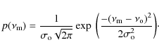
In fact, we subsequently ignore the normalization factor,
As with the ![]() method,
we search our grid of models for model(s) whose frequencies fit the
observed frequencies best, but in this case we are looking for the
highest probability rather than the lowest
method,
we search our grid of models for model(s) whose frequencies fit the
observed frequencies best, but in this case we are looking for the
highest probability rather than the lowest ![]() .
In the Bayesian approach, though, we can assign an overall probability of the model M matching the observed frequencies with respect to the entire set of models according to Bayes' theorem as
.
In the Bayesian approach, though, we can assign an overall probability of the model M matching the observed frequencies with respect to the entire set of models according to Bayes' theorem as
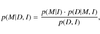
where
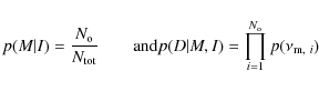
are the uniform prior probability for a specific model and the likelihood function, respectively. For the former we use the percentage of the total number of observed frequencies (
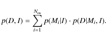
The likelihood function is the ``and'' probability of the individual
probabilities of the most credible model frequencies, which were
identified in the search for the best model fit. In other words,
p(D; M, I) is the probability that
![]() fit the corresponding observed frequencies.
fit the corresponding observed frequencies.
The overall model probability is a very sensitive tool because a high
probability is only assigned if (almost) all observed frequencies can
be matched well. It has to be mentioned that in practice we allow a
model frequency to be assigned to more than one observed frequency.
This is especially important for example with rotational split modes
where several observed modes need to be matched to a single-mode
frequency, since the models do not include rotationally split modes.
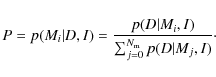
The denominator of Eq. (3) is a normalization factor for the specific model probability in the form of
Since the uniform priors are the same for all models they cancel in Eq. (3), which simplifies to
The resulting model probability distribution in the model space shows regions of highest probability in contrast to others. This automatically translates into uncertainties in the fundamental parameters of the stellar models by constructing the marginal distribution of the corresponding model parameter. The normalized probability of the most probable model is therefore a measure of how likely this model is with respect to the other models of the specific grid. We stress that it does not tell us how probable the model fit is in an absolute sense. The probability is restricted to the space of the models being considered and their associated physics.
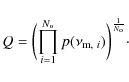
When comparing solutions of different fits (e.g., for different model
grids, or using different sets of observed frequencies) a more robust
value for the ``quality of the fit'' is the geometric mean of the
frequency probabilities (Eq. (2)) of the best fitting model:
The best-fit model identified by the Bayesian approach is the same model as that identified by the
![\begin{figure}
\par\includegraphics[width=9cm,clip]{11438fig6.eps} \vspace*{5mm}
\end{figure}](/articles/aa/full_html/2010/02/aa11438-08/img76.png)
|
Figure 5:
The cumulative probability distribution functions for the effective
temperature and luminosity of the solar calibrated grid. The dotted
lines correspond to the median and the dashed lines give the
|
| Open with DEXTER | |
Using the ![]() -method to find a best fit between model and observed frequencies we found a ridge of models with
-method to find a best fit between model and observed frequencies we found a ridge of models with ![]() below a given threshold, which are basically located on a contour with
a constant large frequency separation where the ridge spans quite a
wide range in temperature and luminosity (of course depending on the
chosen threshold). The model parameters cannot be constrained in an
objective manner.
below a given threshold, which are basically located on a contour with
a constant large frequency separation where the ridge spans quite a
wide range in temperature and luminosity (of course depending on the
chosen threshold). The model parameters cannot be constrained in an
objective manner.
As an example, in Fig. 5
we show the cumulative (i.e., integrated or summed) probability
distribution functions of the models as a function of effective
temperature and luminosity, respectively. From them, we can derive the
most probable model parameters and their uncertainties as, e.g. the
median and the
![]() environment. The latter refer to a Gaussian error distribution and can
easily be replaced by, e.g. a confidence interval. The cumulative
probability distribution functions, however, yields a most probable
effective temperature and luminosity of
environment. The latter refer to a Gaussian error distribution and can
easily be replaced by, e.g. a confidence interval. The cumulative
probability distribution functions, however, yields a most probable
effective temperature and luminosity of ![]() K and
K and
![]() ,
respectively. If the frequency uncertainties were larger, than the high
probability would be distributed amongst more models leading to a
shallower cumulative probability distribution, and the uncertainties of
the model parameters would be larger. The uncertainties are not the
uncertainties within which we can determine HD 49933's position in
the HD-diagram, but they instead correspond to the uncertainties within
which we can constrain the model parameters within a given grid.
The uncertainties appear unrealistically small because we have not
included any assumptions about the model uncertainties themselves.
,
respectively. If the frequency uncertainties were larger, than the high
probability would be distributed amongst more models leading to a
shallower cumulative probability distribution, and the uncertainties of
the model parameters would be larger. The uncertainties are not the
uncertainties within which we can determine HD 49933's position in
the HD-diagram, but they instead correspond to the uncertainties within
which we can constrain the model parameters within a given grid.
The uncertainties appear unrealistically small because we have not
included any assumptions about the model uncertainties themselves.
By applying the Bayesian method to the metal-poor model grid, we find the best model fit (identical to the ![]() best model) has an overall probability of about 0.39 and a quality of the fit of
best model) has an overall probability of about 0.39 and a quality of the fit of ![]() 0.043.
Interestingly, the overall probability of the best fitting model is
higher for the metal-poor grid than for the solar one. One cannot
conclude that the metal-poor grid fit is better because the best
fitting probability is a measure of the probability of the best-fit
model compared to all the other models in its grid and not to the other
models' grid. To directly compare the fits of different grids it is
necessary to compute the global likelihood, i.e. the sum of the
individual model probabilities from each grid. This is done in the
following way.
0.043.
Interestingly, the overall probability of the best fitting model is
higher for the metal-poor grid than for the solar one. One cannot
conclude that the metal-poor grid fit is better because the best
fitting probability is a measure of the probability of the best-fit
model compared to all the other models in its grid and not to the other
models' grid. To directly compare the fits of different grids it is
necessary to compute the global likelihood, i.e. the sum of the
individual model probabilities from each grid. This is done in the
following way.
The probability that grid A provides better model fits to a given set
of frequencies than grid B (assuming that the models themselves are
correct) is given by
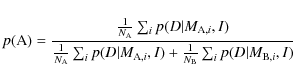
with
Even though the new approach yields excellent results in the present case, it is very sensitive to the presence of artifacts, i.e., if some of the observed frequencies are not intrinsic to the star, then the Bayesian approach will (correctly) not identify any models as being probable. This is not an issue for the modes we identified for HD 49933 in Paper I, but can be a problem for other analyses with lower quality data sets. From Eq. (4) it can be seen that a single observed frequency that does not come close to a model frequency (and consequently has a very low probability of being matched by one of the model frequencies) pushes the overall model probability close to zero. This in turn justifies our very conservative frequency determination described in Paper I. In Gruberbauer et al. (in prep.) we will present a modified version of the algorithm that takes possible artifacts into account.
4 Conclusions
In Paper I we used a Bayesian approach to determine pulsation frequencies of HD 49933 in photometric data obtained by CoRoT. In this paper we have introduced a probability, based on Bayesian methodology, to quantify how closely a model matches the observed pulsation frequency spectrum within uncertainties, compared to other models in a dense and extensive grid of model oscillation spectra.We obtained the following results from our analysis.
- 1.
- We first compared the 26 frequencies to model oscillation spectra in our solar composition grid. We identified a best fit with
 0.79 using nonadiabatic frequencies. The luminosity and effective
temperature of the best model fit lies within the uncertainty box for
HD 49933 in the H-R diagram. The mass, age, and radius of the best
model fit is
0.79 using nonadiabatic frequencies. The luminosity and effective
temperature of the best model fit lies within the uncertainty box for
HD 49933 in the H-R diagram. The mass, age, and radius of the best
model fit is
 ,
2.15 Gyr, and
,
2.15 Gyr, and
 .
.
- 2.
- Owing to the uncertain interior metal abundance, we repeated the search with a lower Y and Z grid of models,
(Y, Z) = (0.24, 0.008). We identified a best fit with
 .
The luminosity and effective temperature of the best-fit model lie
outside the uncertainty box in the HR diagram for HD 49933.
.
The luminosity and effective temperature of the best-fit model lie
outside the uncertainty box in the HR diagram for HD 49933.
- 3.
- We used a Bayesian approach to assign a probability to the model fits and confirmed that the solar Z fit is significantly more probable than the low Z model fit, assuming that the models themselves are valid.
- 4.
- We showed that the mode identification of Appourchaux et al. (2008) yields significantly higher
values than our mode identification.
- 5.
- We showed that the adiabatic and nonadiatic frequencies yield nearly identical model fits to the observed modes. For the Sun it is known that the nonadiabatic effect accounts for a large portion of the surface layer effect. We therefore conclude that the deficiencies in modeling the stellar surface layers only have weak effects on the present analysis.
The frequency extraction by Appourchaux et al. (2008) yielded some frequencies that they interpreted as l = 2 modes or rotational split components. Our more conservative analysis does not yield any evidence for frequencies of higher order than l = 1. When we looked for statistically significant modes adjacent to the well-identified modes, we could not find any evidence for additional modes or rotational split components. We suggest that possibly the a priori assumption by Appourchaux et al. (2008) that the l = 0, 1, and 2 modes have a fixed ratio of heights may have led to spurious l = 2 mode identifications. Likewise, we came to a different mode identification than Appourchaux et al. (2008).
Our estimates of the surface abundances of Fe, C, and O reveal that Fe
is under abundant compared to the Sun and that C and O have near solar
abundances. Owing to this ambiguity we fit the observed frequencies to
both a solar composition grid and a low Z grid. The convective envelope mass of the best-fit model in the solar composition grid is
![]() .
.
We note that the abundances of both helium and heavy elements in HD 49933's thin convective envelope will be affected by diffusion processes such as gravitational settling and radiative levitation. Because of computational difficulties we do not follow element diffusion when the envelope thins below 0.1% of the star's total mass. The mixed metal abundances at the surface make this star an excellent candidate for detailed modeling that includes Y and Z diffusion. A key question we hope to address in a future paper is, whether we can distinguish and isolate the effects of diffusion, metal abundance, helium abundance, and mixing length parameter.
We introduced a Bayesian approach to define a probability that
the observed frequencies match a given model spectrum within a grid of
model eigenspectra. The model probability allows one to compare
distinct model fits with each other, something that the normalized ![]() values cannot do. Although our analysis of HD 49933 has yielded
results that appear to be more consistent with non-asteroseismic data
than the Appourchaux et al. (2008)
results, we do not consider this to be the final word on the subject
and fully expect that HD 49933 will provide us with new
information about Procyon-like stars. We look to future asteroseismic
analyses of the CoRoT data to determine the depth of HD 49933's
convective envelope, to determine its helium abundance, to confirm its
location in the H-R diagram and phase of evolution, and to test models
of Y and Z diffusion. Where seismologists had difficulty
trying to interpret the tentatively identified frequencies in Procyon,
a star similar to HD 49933, CoRoT's observations of HD 49933
are of such high quality that we will soon begin testing the models
themselves.
values cannot do. Although our analysis of HD 49933 has yielded
results that appear to be more consistent with non-asteroseismic data
than the Appourchaux et al. (2008)
results, we do not consider this to be the final word on the subject
and fully expect that HD 49933 will provide us with new
information about Procyon-like stars. We look to future asteroseismic
analyses of the CoRoT data to determine the depth of HD 49933's
convective envelope, to determine its helium abundance, to confirm its
location in the H-R diagram and phase of evolution, and to test models
of Y and Z diffusion. Where seismologists had difficulty
trying to interpret the tentatively identified frequencies in Procyon,
a star similar to HD 49933, CoRoT's observations of HD 49933
are of such high quality that we will soon begin testing the models
themselves.
T.K., M.G., L..F, and W.W.W. are supported by the Austrian Research Promotion Agency (FFG), and the Austrian Science Fund (FWF P17580). T.K. is also supported by the Canadian Space Agency. D.B.G. acknowledges the support of the Natural Sciences and Engineering Research Council of Canada.
References
- Alexander, D. R., & Ferguson, J. W. 1994, ApJ, 437, 879 [NASA ADS] [CrossRef] [Google Scholar]
- Appourchaux, T., Michel, E., Auvergne, M., et al. 2008, A&A, 488, 705 [NASA ADS] [CrossRef] [EDP Sciences] [Google Scholar]
- Baglin, A., Michel, E., Auvergne, M., et al. 2006, in ESA SP, 1306, 39 [Google Scholar]
- Bazot, M., Bourguignon, S., & Christensen-Dalsgaard, J. 2008, Mem. Soc. Astron. Ital., 79, 660 [Google Scholar]
- Blackwell, D. E., & Lynas-Gray, A. E. 1998, A&AS, 129, 505 [Google Scholar]
- Böhm-Vitense, E. 1958, Zeitschrift fur Astrophysik, 46, 108 [Google Scholar]
- Boisnard, L., & Auvergne. 2006, in ESA SP, 1306, 19 [Google Scholar]
- Bruntt, H., De Cat, P., & Aerts, C. 2008, A&A, 478, 487 [NASA ADS] [CrossRef] [EDP Sciences] [Google Scholar]
- Chaplin, W. J., Houdek, G., Elsworth, Y., et al. 2005, MNRAS, 360, 859 [NASA ADS] [CrossRef] [Google Scholar]
- Demarque, P., Guenther, D. B., & Kim, Y. 1999, ApJ, 517, 510 [NASA ADS] [CrossRef] [Google Scholar]
- Fuhrmann, K., Pfeiffer, M., Frank, C., Reetz, J., & Gehren, T. 1997, A&A, 323, 909 [NASA ADS] [Google Scholar]
- Gillon, M., & Magain, P. 2006, A&A, 448, 341 [NASA ADS] [CrossRef] [EDP Sciences] [Google Scholar]
- Grevesse, N., Noels, A., & Sauval, A. J. 1996, in Cosmic Abundances, ed. S. S. Holt, & G. Sonneborn, ASP Conf. Ser., 99, 117 [Google Scholar]
- Gruberbauer, M., Kallinger, T., Weiss, W. W., & Guenther, D. B. 2009, A&A, 506, 1043 [NASA ADS] [CrossRef] [EDP Sciences] [Google Scholar]
- Guenther, D. B. 1994, ApJ, 422, 400 [NASA ADS] [CrossRef] [Google Scholar]
- Guenther, D. B., & Brown, K. I. T. 2004, ApJ, 600, 419 [NASA ADS] [CrossRef] [Google Scholar]
- Guenther, D. B., Demarque, P., Kim, Y.-C., & Pinsonneault, M. H. 1992, ApJ, 387, 372 [NASA ADS] [CrossRef] [Google Scholar]
- Guenther, D. B., Kim, Y., & Demarque, P. 1996, ApJ, 463, 382 [NASA ADS] [CrossRef] [Google Scholar]
- Guenther, D. B., Kallinger, T., Reegen, P., et al. 2005, ApJ, 635, 547 [NASA ADS] [CrossRef] [Google Scholar]
- Iglesias, C. A., & Rogers, F. J. 1996, ApJ, 464, 943 [NASA ADS] [CrossRef] [Google Scholar]
- Jørgensen, B. R., & Lindegren, L. 2005, A&A, 436, 127 [NASA ADS] [CrossRef] [EDP Sciences] [Google Scholar]
- Kallinger, T., Guenther, D. B., Matthews, J. M., et al. 2008, A&A, 478, 497 [NASA ADS] [CrossRef] [EDP Sciences] [Google Scholar]
- Kjeldsen, H., Bedding, T. R., & Christensen-Dalsgaard, J. 2008, ApJ, 683, L175 [NASA ADS] [CrossRef] [Google Scholar]
- Kochukhov, O. P. 2007, in Physics of Magnetic Stars, 109 [Google Scholar]
- Kupka, F., Piskunov, N., Ryabchikova, T. A., Stempels, H. C., & Weiss, W. W. 1999, A&AS, 138, 119 [NASA ADS] [CrossRef] [EDP Sciences] [MathSciNet] [PubMed] [Google Scholar]
- Lejeune, T., & Schaerer, D. 2001, A&A, 366, 538 [NASA ADS] [CrossRef] [EDP Sciences] [Google Scholar]
- Moon, T. T., & Dworetsky, M. M. 1985, MNRAS, 217, 305 [NASA ADS] [CrossRef] [Google Scholar]
- Piskunov, N. E., Kupka, F., Ryabchikova, T. A., Weiss, W. W., & Jeffery, C. S. 1995, A&AS, 112, 525 [Google Scholar]
- Rogers, F. J. 1986, ApJ, 310, 723 [NASA ADS] [CrossRef] [Google Scholar]
- Rogers, F. J., Swenson, F. J., & Iglesias, C. A. 1996, ApJ, 456, 902 [NASA ADS] [CrossRef] [Google Scholar]
- Roxburgh, I. W. 2005, A&A, 434, 665 [NASA ADS] [CrossRef] [EDP Sciences] [Google Scholar]
- Roxburgh, I. W., & Vorontsov, S. V. 2000, MNRAS, 317, 141 [NASA ADS] [CrossRef] [Google Scholar]
- Roxburgh, I. W., & Vorontsov, S. V. 2001, MNRAS, 322, 85 [NASA ADS] [CrossRef] [Google Scholar]
- Roxburgh, I. W., & Vorontsov, S. V. 2003, A&A, 411, 215 [NASA ADS] [CrossRef] [EDP Sciences] [Google Scholar]
- Ryabchikova, T., Fossati, L., & Shulyak, D. 2009, A&A, 506, 203 [NASA ADS] [CrossRef] [EDP Sciences] [Google Scholar]
- Ryabchikova, T. A., Piskunov, N. E., Stempels, H. C., Kupka, F., & Weiss, W. W. 1999, Phys. Scr., T 83, 162 [Google Scholar]
- Shulyak, D., Tsymbal, V., Ryabchikova, T., Stütz, C., & Weiss, W. W. 2004, A&A, 428, 993 [NASA ADS] [CrossRef] [EDP Sciences] [Google Scholar]
- van Leeuwen, F. 2007, A&A, 474, 653 [NASA ADS] [CrossRef] [EDP Sciences] [Google Scholar]
- Vitense, E. 1953, Z. Astrophys., 32, 135 [NASA ADS] [Google Scholar]
Footnotes
- ...CoRoT
- The CoRoT space mission was developed and is operated by the French space agency CNES, with participation of ESA's RSSD and Science Pograms, Austria, Belgium, Brazil, Germany, and Spain.
All Tables
Table 1: Summary of the best fitting solar-abundance and metal-poor adiabatic and nonadiabatic models for the frequencies given by A: Gruberbauer et al. (2009) and B: Appourchaux et al. (2008).
All Figures
|
|
Figure 1:
Observed H |
| Open with DEXTER | |
| In the text | |
|
|
Figure 2: Top panel: echelle diagram of the observed oscillation frequencies and the adiabatic and nonadiabatic eigenfrequencies of the best fitting model from the solar abundance model grid. The observed frequencies are shown as filled circles with the error bars indicating the observational uncertainties. The nonadiabatic model frequencies used in the analysis are displayed with gray symbols connected by line segments. The adiabatic frequencies are indicated by line segments only. Bottom panel: same as above, but for the best fitting metal-poor model. |
| Open with DEXTER | |
| In the text | |
|
|
Figure 3: Top panel: difference between the adiabatic and nonadiabatic eigenfrequencies for the l = 0 and 1 modes of the best fitting solar-abundance model and the frequency difference between the observed and nonadiabatic frequencies. Black dots indicate the differences between the observed and the nonadiabatic frequencies with error bars for the observations. Bottom panel: similar to above except showing the Appourchaux et al. (2008) frequencies and uncertainties. |
| Open with DEXTER | |
| In the text | |
|
|
Figure 4:
Theoretical H-R diagram showing the uncertainty box of HD 49933
and a subset of the solar abundance stellar model grid (light gray
dots). The color scale (in the online version only) gives the |
| Open with DEXTER | |
| In the text | |
|
|
Figure 5:
The cumulative probability distribution functions for the effective
temperature and luminosity of the solar calibrated grid. The dotted
lines correspond to the median and the dashed lines give the
|
| Open with DEXTER | |
| In the text | |
Copyright ESO 2010
Current usage metrics show cumulative count of Article Views (full-text article views including HTML views, PDF and ePub downloads, according to the available data) and Abstracts Views on Vision4Press platform.
Data correspond to usage on the plateform after 2015. The current usage metrics is available 48-96 hours after online publication and is updated daily on week days.
Initial download of the metrics may take a while.