| Issue |
A&A
Volume 509, January 2010
|
|
|---|---|---|
| Article Number | A10 | |
| Number of page(s) | 12 | |
| Section | Extragalactic astronomy | |
| DOI | https://doi.org/10.1051/0004-6361/20078239 | |
| Published online | 12 January 2010 | |
The distance to the C component of I Zw 18 and its star formation history
A probabilistic approach
L. Jamet1,2 - M. Cerviño1 - V. Luridiana1,3 - E. Pérez1 - T. Yakobchuk4
1 - Instituto de Astrofísica de Andalucía (CSIC), Camino bajo de Huétor, 50, Granada 18080, Spain
2 - Instituto de Astronomía, Universidad Nacional Autónoma de
México, Apartado Postal 70-264, Ciudad Universitaria, México D.F.
04510, Mexico
3 -
Instituto de Astrofísica de Canarias (IAC), c/Vía Láctea s/n, La Laguna, 38205 Tenerife, Spain
4 -
Main Astronomical Observatory, Zabolotnoho 27, Kyiv 03680, Ukraine
Received 7 July 2007 / Accepted 20 August 2009
Abstract
Aims. We analyzed the resolved stellar population of the C
component of the extremely metal-poor dwarf galaxy I Zw18 in
order to evaluate its distance and star formation history as accurately
as possible. In particular, we aimed at answering the question of
whether this stellar population is young.
Methods. We developed a probabilistic approach to analyzing
high-quality photometric data obtained with the Advanced Camera for
Surveys of the Hubble Space Telescope. This approach gives a detailed
account of the various stochastic aspects of star formation. We carried
out two successive models of the stellar population of interest, paying
attention to how our assumptions could affect the results.
Results. We found a distance to the C component of I Zw 18 as
high as 27 Mpc, a significantly higher value than those cited in
previous works. The star formation history we inferred from the
observational data shows various interesting features: a strong
starburst that lasted for about 15 Myr, a more moderate one that
occurred ![]() 100 Myr
ago, a continuous process of star formation between both starbursts,
and a possible episode of low level star formation at ages over
100 Myr. The stellar population studied is likely
100 Myr
ago, a continuous process of star formation between both starbursts,
and a possible episode of low level star formation at ages over
100 Myr. The stellar population studied is likely ![]() 125 Myr
old, although ages of a few Gyr cannot be ruled out. Furthermore,
nearly all the stars were formed in the last few hundreds of Myr.
125 Myr
old, although ages of a few Gyr cannot be ruled out. Furthermore,
nearly all the stars were formed in the last few hundreds of Myr.
Key words: galaxies: individual: I Zw 18 - galaxies: photometry - galaxies: stellar content - galaxies: formation
1 Introduction
The study of dwarf galaxies is an important topic for the understanding of how galaxies form and evolve. Their presence in galaxy clusters and their physical properties put constraints on cosmological models, especially on the dark matter content of the Universe (e.g. Robertson et al. 2005). Furthermore, because their shallow gravitational potential well, dwarf irregular (dIrr) galaxies are ideal benchmarks for studing the effects of various processes, either internal (e.g., stellar winds and supernovae) or external (like gas infall and tidal forces), on the triggering and regulation of star formation (SF) in galaxies (Hunter et al. 1998; Hensler & Rieschick 2002). Finally, metal-deficient dIrr galaxies are expected to match the chemical composition of pristine galaxies, and efforts have been made to derive the primordial helium abundance of the Universe from the spectroscopic analysis of their ionized gas (Peimbert & Torres-Peimbert 1974, 1976; Izotov et al. 1997b, 2007; Peimbert et al. 2007).
Among the dIrr galaxies known, I Zw18 is arguably the
most fascinating one. This object is the second lowest
metallicity galaxy known (12 + log O/H = 7.2), corresponding
to ![]() 1/30 of the solar value (e.g. Pagel et al. 1992; Skillman & Kennicutt 1993; Izotov & Thuan 1998; Izotov et al. 1999), being the lowest one SBS 0335-052 (West) (Izotov et al. 2004).
Its blue color (van Zee et al. 1998) and its intense
nebular emission (e.g. Vílchez & Iglesias-Páramo 1998; Cannon et al. 2002)
bears witness to an intense ongoing SF episode. The galaxy presents a complex
morphology; it is dominated by a two-lobed body (the ``main
body'') with one companion,
the ``C component'' (hereafter I Zw18 Dufour et al. 1996a).
1/30 of the solar value (e.g. Pagel et al. 1992; Skillman & Kennicutt 1993; Izotov & Thuan 1998; Izotov et al. 1999), being the lowest one SBS 0335-052 (West) (Izotov et al. 2004).
Its blue color (van Zee et al. 1998) and its intense
nebular emission (e.g. Vílchez & Iglesias-Páramo 1998; Cannon et al. 2002)
bears witness to an intense ongoing SF episode. The galaxy presents a complex
morphology; it is dominated by a two-lobed body (the ``main
body'') with one companion,
the ``C component'' (hereafter I Zw18 Dufour et al. 1996a).
In spite of many efforts, the distance and, more important,
the age of the galaxy have not been well determined yet. By analyzing
HST/WFPC2 color-magnitude diagrams (CMDs) and
HST/FOS spectra, and assuming a distance of 10 Mpc (applying
straightly the Hubble law to the redshift of the galaxy),
Dufour et al. (1996b) detected a stellar
population of up to 50 Myr in the main body of the galaxy and up
to 300 Myr in the C component. They found no support for or
against an old underlying population. Assuming the same distance and
examining a larger set of HST/WFPC2 photometric
data, Aloisi et al. (1999) decomposed the star formation history
(SFH) in a continuous SF lasting over ![]() 1 Gyr and an ongoing
starburst that started
1 Gyr and an ongoing
starburst that started ![]() 15-20 Myr ago. By analyzing
HST/WFPC2 CMDs jointly, ground-based spectra and the morphology
of some nebular features, Izotov et al. (1999) find
that a distance of 20 Mpc is necessary to explain the ionization
state of the gas. They also state that the age of the galaxy,
as derived from all three kinds of data, does not exceed 100 Myr, in agreement with the conclusion from Izotov & Thuan (1999) that very metal-deficient galaxies must all be young.
Östlin (2000) carried out an analysis of HST/NICMOS photometric
data and detected asymptotic giant branch stars (AGB) that,
at the adopted distance of 12.6 Mpc (derived from the redshift
corrected for the Virgocentric flow), are at least 1 Gyr old. From
the surface distribution of the fluxes and colors of the galaxy,
Kunth & Östlin (2000) argue that I Zw18 is an old galaxy whose age is likely
15-20 Myr ago. By analyzing
HST/WFPC2 CMDs jointly, ground-based spectra and the morphology
of some nebular features, Izotov et al. (1999) find
that a distance of 20 Mpc is necessary to explain the ionization
state of the gas. They also state that the age of the galaxy,
as derived from all three kinds of data, does not exceed 100 Myr, in agreement with the conclusion from Izotov & Thuan (1999) that very metal-deficient galaxies must all be young.
Östlin (2000) carried out an analysis of HST/NICMOS photometric
data and detected asymptotic giant branch stars (AGB) that,
at the adopted distance of 12.6 Mpc (derived from the redshift
corrected for the Virgocentric flow), are at least 1 Gyr old. From
the surface distribution of the fluxes and colors of the galaxy,
Kunth & Östlin (2000) argue that I Zw18 is an old galaxy whose age is likely ![]() 5 Gyr. A significant age of possibly several Gyr has also been advocated by Legrand et al. (2000) to account
for the very homogeneous distribution of heavy elements
throughout the ionized, optical-emitting gas of the galaxy. By
studying the deep spectra of I Zw18C, Izotov et al. (2001) find
that a distance of
5 Gyr. A significant age of possibly several Gyr has also been advocated by Legrand et al. (2000) to account
for the very homogeneous distribution of heavy elements
throughout the ionized, optical-emitting gas of the galaxy. By
studying the deep spectra of I Zw18C, Izotov et al. (2001) find
that a distance of ![]() 15 Mpc
is needed to reconcile ionized gas in this object with the apparent
magnitudes of its brightest blue stars. This distance can actually be
interpreted as
a lower limit, since at larger distances these stars would be still
considered as ionizing. Their spectra are well-fitted by models
with a continuous star formation extending over the past
10-100 Myr, with no evidence of any older underlying stellar
population. Papaderos et al. (2002) compared surface brightness
maps obtained through various optical and near-infrared filters
with the HST, which did not reveal any stellar population older
than 0.5 Gyr. Such a population may exist, but most of the stellar
content must be younger than this age. Izotov & Thuan (2004)
carried out deep HST/ACS observations of I Zw18, improving
by
15 Mpc
is needed to reconcile ionized gas in this object with the apparent
magnitudes of its brightest blue stars. This distance can actually be
interpreted as
a lower limit, since at larger distances these stars would be still
considered as ionizing. Their spectra are well-fitted by models
with a continuous star formation extending over the past
10-100 Myr, with no evidence of any older underlying stellar
population. Papaderos et al. (2002) compared surface brightness
maps obtained through various optical and near-infrared filters
with the HST, which did not reveal any stellar population older
than 0.5 Gyr. Such a population may exist, but most of the stellar
content must be younger than this age. Izotov & Thuan (2004)
carried out deep HST/ACS observations of I Zw18, improving
by ![]() 2 mag the depth of stellar photometric data with respect
to previous efforts. They concludes that the distance to I Zw18
should lie somewhere between 12.6 and 15 Mpc with the latter
value being more likely, and claim that the absence of any
detected red giant is proof that the galaxy is young (
2 mag the depth of stellar photometric data with respect
to previous efforts. They concludes that the distance to I Zw18
should lie somewhere between 12.6 and 15 Mpc with the latter
value being more likely, and claim that the absence of any
detected red giant is proof that the galaxy is young (![]() 500 Myr). Finally, by analyzing the same images as Izotov & Thuan (2004), along with other deep HST/ACS data, Aloisi et al. (2007) detected a red giant branch (RGB), as well as a confirmed,
Cepheid star. They derived a distance of
500 Myr). Finally, by analyzing the same images as Izotov & Thuan (2004), along with other deep HST/ACS data, Aloisi et al. (2007) detected a red giant branch (RGB), as well as a confirmed,
Cepheid star. They derived a distance of ![]() 18 Mpc and
argue that the presence of RBG stars shows that the galaxy is
old (at least 1 Gyr, but see also Tosi et al. 2007).
18 Mpc and
argue that the presence of RBG stars shows that the galaxy is
old (at least 1 Gyr, but see also Tosi et al. 2007).
It is striking to see that similar approaches to the evaluation
of the age of I Zw18 lead to contradictory results (e.g.,
Dufour et al. 1996b vs. Aloisi et al. 1999; or Kunth & Östlin 2000 vs. Papaderos et al. 2002). It turns out that the age estimates from the authors mentioned above go from a ten
Myr to several Gyr! This might be explained at least partially by
some uncertainties in the studies summarized above, such as the
limited depth of the available data or the sensitivity of CMD
analysis to the distance and extinction adopted. For this reason,
we decided to carry out a new analysis of the deep HST/ACS
observations performed by Izotov & Thuan (2004), focusing
on I Zw18C. The latter has been little studied because of
its faintness (![]() 24 mag/
24 mag/
![]() in the V band).
However, there is a key difference between I Zw 18C and the main body
that makes the C component more attractive for CMD studies: it is
older.
in the V band).
However, there is a key difference between I Zw 18C and the main body
that makes the C component more attractive for CMD studies: it is
older.
- 1.
- There is a significant absence of nebular emission. Because it is older, the observed surface brightness in the C component is lower than in the main body and is predominantly produced by the stellar component. The surface brightness in the main body is produced by both the stellar and nebular components (see, e.g. Vílchez & Iglesias-Páramo 1998). Also, compact clumps of ionized gas in the main component would mimic stellar sources, and the patchy ionized gas emission makes background subtraction more difficult.
- 2.
- Isochrones (and their associated stellar luminosity functions) have a simpler structure at older (post Wolf-Rayet) ages, with well-defined structures excepting the blue loops that make a small contribution in the stellar luminosity function. In the case of the main component, there are identified Wolf-Rayet stars (Legrand et al. 1997; Izotov et al. 1997a) such a presence is difficult to explain in low-metallicity environment with standard evolutionary models Brown et al. (2002), so more complex evolutionary models (like the inclusion of rotation) would be required. However, current models including rotation produce evolutionary tracks with complex structures (see e.g. Fig. 3 in Meynet & Maeder 2005), so isochrones becomes strongly dependent on the assumed initial rotational velocity, the possible distribution of rotational velocities, and the (still unexplored) validity of homology relations between different stellar tracks for rotating stars.
For these reasons, we have decided to use study I Zw18C instead of the main body. We had built a new, improved CMD from the images of Izotov & Thuan (2004) and analyzed it with a probabilistic approach to evaluate the distance, the SFH, and the age of this component.
This paper is divided as follows. In Sect. 2, we define the probabilistic tools used in our approach. In Sect. 3, we describe the observational data and the theoretical isochrones on which our work was based. In Sect. 4, we present a first model of the stellar population studied. Section 5 is dedicated to a revision of the assumptions of this model, and in Sect. 6 we present a new model with improved reliability. We infer the minimum age of I Zw18C and discuss the estimate of its distance. Finally, we give our conclusions in Sect. 7.
2 A probabilistic approach
In considering a stellar population in which N individual stars
are detected in a set of n photometric bands, note mi,jthe magnitude of the jth star in the ith photometric band. We
first examine the case of a simple stellar population, i.e. a population
where all the stars were formed at the same time and in
the same conditions. The initial mass
![]() of the jth star is considered
a random variable and the initial mass function (IMF)
of the jth star is considered
a random variable and the initial mass function (IMF)
![]() is regarded as the probability density function (PDF) from
which
is regarded as the probability density function (PDF) from
which
![]() is drawn. The expected magnitudes
is drawn. The expected magnitudes
![]() of the star
depend on
of the star
depend on
![]() and on properties of the stellar
population: the age
and on properties of the stellar
population: the age ![]() ,
the metallicity Z, the distance d and the
interstellar extinction coefficients Ai. Furthermore, those magnitudes
are affected by photometric errors, which we suppose
follow Gaussian distributions of widths
,
the metallicity Z, the distance d and the
interstellar extinction coefficients Ai. Furthermore, those magnitudes
are affected by photometric errors, which we suppose
follow Gaussian distributions of widths
![]() .
Finally,
the photometric data do not usually cover the whole IMF of
the stellar population, since the faintest stars are not detected.
Consequently, if we call
.
Finally,
the photometric data do not usually cover the whole IMF of
the stellar population, since the faintest stars are not detected.
Consequently, if we call
![]() the photometric completeness
function of the data (the probability a star of magnitudes miis detected), then the observed magnitudes mi,j of the star jare associated to the following likelihood function (LF):
the photometric completeness
function of the data (the probability a star of magnitudes miis detected), then the observed magnitudes mi,j of the star jare associated to the following likelihood function (LF):
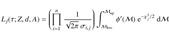
with
and
In Eqs. (1) and (2), the upper limit
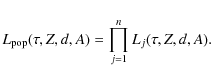
Assuming that the initial masses of the stars are mutually
independent, the LF
![]() associated to the distribution of magnitudes
of the N stars is given by the product of the individual LFs Lj:
associated to the distribution of magnitudes
of the N stars is given by the product of the individual LFs Lj:
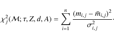
In practice, it is preferable to work not with the LFs themselves, but rather with their logarithms. Hence, we introduce the following quantities:

In this section, we have limited the definition of Lj to the case of a simple stellar population. In what follows, we propose another definition that can be applied to composite populations.
2.1 Introducing the stellar formation history into the entropy
Many stellar populations show prolonged periods of star formation,
in which case Eq. (1) cannot be used. It is necessary to introduce
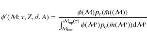
a function
![]() that describes the SFH of the population studied.
Like their initial masses, the ages of the different stars are
supposed to be independent random variables. As a result, we define
that describes the SFH of the population studied.
Like their initial masses, the ages of the different stars are
supposed to be independent random variables. As a result, we define
![]() as the expectancy of the number of stars observable
today and whose ages are comprised between
as the expectancy of the number of stars observable
today and whose ages are comprised between ![]() and
and
![]() .
Consequently,
.
Consequently,
![]() must be replaced by the following LF:
must be replaced by the following LF:
with
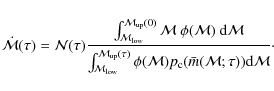
The entropy
For given values of Z, d, and A, maximizing
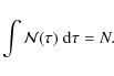
The mass rate
In some cases, a parametric model can be provided for the SFH. In this case,
2.2 Comparison with other approaches
The variable
![]() is an entropic tool whose maximization can be used to
analyze resolved stellar populations. Contrary to simpler estimators
(e.g., the chi-square one), it is sensitive not only to the
shape of the tested isochrones in color-magnitude diagrams,
but also to the density distribution of the stars along those
isochrones, through the relations between the age, mass and
magnitudes. This is particularly true for rapid stellar phases,
where the magnitudes are very sensitive to the ages and initial
masses of the stars. Other probabilistic methods have been
developed to characterize resolved stellar populations,
especially the comparison of star counts between observed and
synthetic Monte-Carlo CMDs in different bins of the color-magnitude
space (e.g. Gallart et al. 1999). However, the formalism
proposed in this work is based on rigorous concepts,
it is more accurate than the synthetic CMD approach. In
particular, it avoids the biases and errors caused by the binning of
data and the random content of simulated CMDs. Moreover, it
bypasses expensive Monte-Carlo computations for the search
of optimized parameters of the stellar population studied.
In summary,
is an entropic tool whose maximization can be used to
analyze resolved stellar populations. Contrary to simpler estimators
(e.g., the chi-square one), it is sensitive not only to the
shape of the tested isochrones in color-magnitude diagrams,
but also to the density distribution of the stars along those
isochrones, through the relations between the age, mass and
magnitudes. This is particularly true for rapid stellar phases,
where the magnitudes are very sensitive to the ages and initial
masses of the stars. Other probabilistic methods have been
developed to characterize resolved stellar populations,
especially the comparison of star counts between observed and
synthetic Monte-Carlo CMDs in different bins of the color-magnitude
space (e.g. Gallart et al. 1999). However, the formalism
proposed in this work is based on rigorous concepts,
it is more accurate than the synthetic CMD approach. In
particular, it avoids the biases and errors caused by the binning of
data and the random content of simulated CMDs. Moreover, it
bypasses expensive Monte-Carlo computations for the search
of optimized parameters of the stellar population studied.
In summary,
![]() allows
a study of the stellar luminosity function as a whole, with its
correlations among different luminosity bins, instead of only portions
of the luminosity function without correlations among bins.
allows
a study of the stellar luminosity function as a whole, with its
correlations among different luminosity bins, instead of only portions
of the luminosity function without correlations among bins.
The approach we have presented is of course not free of drawbacks. In particular, there is no simple way to assess the goodness-of-fit, and Monte-Carlo simulations may be required to carry out this task (see Sect. 4.3). Furthermore, like other probabilistic methods, the results deeply depend on the input physics, in particular the stellar evolution models and the conversion of stellar parameters to magnitudes. Ideally, different evolutionary tracks and model atmospheres, or empirical magnitude calibrations, should be tested when analyzing an object, at the cost of simplicity and time.
3 Applications to I Zw18C
3.1 The photometric data
![\begin{figure}
\par\includegraphics[width=8.5cm,clip]{08239fig1.eps}
\end{figure}](/articles/aa/full_html/2010/01/aa8239-07/img38.png)
|
Figure 1: HST/ACS image of I Zw18C through the F555W filter. The two clusters ``C'' and ``NW'' mentioned by Izotov & Thuan (2004) are reported. The image display scale is logarithmic. North is up and East to the left. The ``white pixels'' are contaminated pixels that were rejected when performing the photometric measurements. |
| Open with DEXTER | |
![\begin{figure}
\par\includegraphics[width=8.5cm,clip]{08239fig2.eps}
\end{figure}](/articles/aa/full_html/2010/01/aa8239-07/img39.png)
|
Figure 2: Color-magnitude diagram of I Zw18C. The typical error bars as a function of F814W are reported for both the blue and red branches. The two clusters are annotated with open circles. The stars marked with crosses are those we rejected from the useful sample due to their extreme red color.We also report the 90% and 50% completeness limits as dashed lines. |
| Open with DEXTER | |
We carried out photometric measurements of the HST/ACS
images obtained in the bands F555W (![]() V; Fig. 1) and F814W
(
V; Fig. 1) and F814W
(![]() I) by Izotov & Thuan (2004). They performed photometric
analysis of those images, obtaining data significantly deeper
than those of previous works. However, their procedure,
made use of a model point spread function (PSF) that was not
optimal. For this reason, we performed our own measurements
by using the well-suited DOLPHOT/ACS package (Dolphin 2000), which correctly accounts for the pixel undersampling of the instruments and uses accurate model PSFs.
I) by Izotov & Thuan (2004). They performed photometric
analysis of those images, obtaining data significantly deeper
than those of previous works. However, their procedure,
made use of a model point spread function (PSF) that was not
optimal. For this reason, we performed our own measurements
by using the well-suited DOLPHOT/ACS package (Dolphin 2000), which correctly accounts for the pixel undersampling of the instruments and uses accurate model PSFs.
The CMD that we obtained is
shown in Fig. 2. The F555W and F814W magnitudes (hereafter
m555 and m814, respectively) are expressed in the VEGAMAG
system![]() . The CMD contains 965 sources going down to
m555 = 29.8 and
m814 = 29.0. We performed artificial star tests (ASTs)
to assess the quality of the photometric data and evaluate
their completeness. The latter shows a significant improvement
with respect to the measurements of Izotov & Thuan (2004). Not only is the 50% completeness limit improved by nearly 1 mag, but the completeness is also maintained high
closer to this limit (the completeness drop is more ``abrupt'').
Furthermore, we used the ASTs to determine photometric errors
that are more realistic than the default outputs by DOLPHOT/ACS
and to evaluate the possible biases in the magnitudes retrieved.
. The CMD contains 965 sources going down to
m555 = 29.8 and
m814 = 29.0. We performed artificial star tests (ASTs)
to assess the quality of the photometric data and evaluate
their completeness. The latter shows a significant improvement
with respect to the measurements of Izotov & Thuan (2004). Not only is the 50% completeness limit improved by nearly 1 mag, but the completeness is also maintained high
closer to this limit (the completeness drop is more ``abrupt'').
Furthermore, we used the ASTs to determine photometric errors
that are more realistic than the default outputs by DOLPHOT/ACS
and to evaluate the possible biases in the magnitudes retrieved.
We checked whether the stellar fluxes suffer from foreground
Galactic extinction. Whereas the survey of Schlegel et al. (1998) yields a Galactic contribution of
AV = 0.11 to the extinction toward I Zw18, the lower-resolution data of Burstein & Heiles (1982) indicate an extinction as small as
AV = 0.01. Furthermore, an analysis of the nebular H![]() /H
/H![]() line carried out by Cannon et al. (2002) shows that some regions of the
main component of I Zw18 suffer very small extinction, if any.
Consequently, we assumed that the Galactic extinction toward
I Zw18C may be negligible and we did not correct our data for it.
line carried out by Cannon et al. (2002) shows that some regions of the
main component of I Zw18 suffer very small extinction, if any.
Consequently, we assumed that the Galactic extinction toward
I Zw18C may be negligible and we did not correct our data for it.
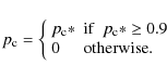
3.2 Selection of the stars
Before carrying out the analysis of I Zw18C, we selected the
stars for use. First, we limited the selection to the
stars situated above the 90% completeness level. This threshold
was chosen for two reasons: (i) the uncertainties in the photometric
analysis (systematic and random errors in the magnitudes,
evaluation of the completeness map) are small for the
region of the CMD selected; and (ii) most of the stars situated
below the 90% completeness limit are main-sequence (MS)
objects that yield little useful information about the age and
distance of the galaxy, compared with post-MS stars. Then,
we rejected the sources situated within the two clusters annotated
as ``C'' and ``NW'' by Izotov & Thuan (2004). Finally, we
removed the five reddest remaining stars from the selection.
According to Marigo & Girardi (2007), who revised the evolutionary
models of asymptotic giant branch (AGB) stars, the
presence of very red stars in the CMD is possible. However,
the characteristics of these objects are still very sensitive to the
physics used to model them. In principle, this problem concerns
only extremely red stars. As a consequence, we decided
to discard the stars with colors
![]() .
The final selection
contains 408 stars, of which 315 are located in the blue
(
.
The final selection
contains 408 stars, of which 315 are located in the blue
(
![]() )
branch and 93 in the red one.
)
branch and 93 in the red one.
Given the selection procedure, the completeness function
![]() for the selected stars can be written as a function of the
``real'' completeness
for the selected stars can be written as a function of the
``real'' completeness
![]() evaluated for the whole CMD:
evaluated for the whole CMD:
3.3 Isochrones
An important assumption of this work regards the isochrones
that we decided to use. We adopted the evolutionary tracks of
Girardi et al. (2000) available for Z = 0.0004 and computed the
theoretical absolute magnitudes through the ACS F555W and
F814W filters![]() using the BaSeL 3.1 stellar library Westera et al. (2002).
using the BaSeL 3.1 stellar library Westera et al. (2002).
4 A first model
4.1 Assumptions and procedure
We proceeded to a first measurement of the distance, extinction, and SFH of I Zw18C. The main assumptions of the calculus were the following:
- a Salpeter IMF (
 )
in the 0.15-120
)
in the 0.15-120
 range;
- the extinction to be uniform over the stellar population. Furthermore, since little work has been done regarding the extinction in I Zw18C (see, however Izotov et al. 2001), we decided to use the extinction AV as a free parameter;
- no constraints on the SFH;
- no concern for the possible effects of binary stars.
4.2 Results
![\begin{figure}
\par\includegraphics[width=8.5cm,clip]{08239fig3.eps}
\end{figure}](/articles/aa/full_html/2010/01/aa8239-07/img59.png)
|
Figure 3:
|
| Open with DEXTER | |
![\begin{figure}
\par\includegraphics[width=8.5cm,clip]{08239fig4.eps}
\end{figure}](/articles/aa/full_html/2010/01/aa8239-07/img60.png)
|
Figure 4:
Observed CMD and theoretical isochrones for the model of
Sect. 4. The observed data are corrected for interstellar extinction, using
the best-fit value
AV = 0.38. The dotted line shows the threshold
above which we selected the stars to work with. The vertical axes
show both apparent and absolute F814W magnitude scales, adopting
the best-fit distance modulus
|
| Open with DEXTER | |
![\begin{figure}
\par\includegraphics[width=8.5cm,clip]{08239fig5.eps}
\end{figure}](/articles/aa/full_html/2010/01/aa8239-07/img61.png)
|
Figure 5: SFH derived from the approached explained in Sect. 4. The curve was slightly smoothed to limit the apparent statistic noise. |
| Open with DEXTER | |
The results are presented as follows. In Fig. 3, we present the
curves of
![]() and
and
![]() .
Figure 4 shows the observed CMD along with some theoretical isochrones for the best-fit
distance modulus and extinction. In Fig. 5, we show the mass
rate
.
Figure 4 shows the observed CMD along with some theoretical isochrones for the best-fit
distance modulus and extinction. In Fig. 5, we show the mass
rate
![]() derived from
derived from
![]() at the best-fit distance and extinction.
at the best-fit distance and extinction.
The best-fit distance modulus is
![]() (corresponding
to a distance of 26.5 Mpc), and the 99.9% confidence interval
for
(corresponding
to a distance of 26.5 Mpc), and the 99.9% confidence interval
for ![]() is 31.71-32.24. Such a distance modulus is higher
than any previous estimate, by >1 mag for most of them and
is 31.71-32.24. Such a distance modulus is higher
than any previous estimate, by >1 mag for most of them and
![]() 0.8 mag for the newest (31.4, Aloisi et al. 2007). As for the
extinction, the best-fit coefficient is
AV = 0.38, and the 99.9%
confidence interval is 0.30-0.45, a higher value than the different
estimates of the foreground Galactic extinction (see Sect. 3.1). This value falls within the 0.20-0.65 interval derived by Izotov et al. (2001) from a spectroscopic study of I Zw18C and
suggests the existence of dust clouds responsible for extinction
inside this object.
0.8 mag for the newest (31.4, Aloisi et al. 2007). As for the
extinction, the best-fit coefficient is
AV = 0.38, and the 99.9%
confidence interval is 0.30-0.45, a higher value than the different
estimates of the foreground Galactic extinction (see Sect. 3.1). This value falls within the 0.20-0.65 interval derived by Izotov et al. (2001) from a spectroscopic study of I Zw18C and
suggests the existence of dust clouds responsible for extinction
inside this object.
The estimate of
![]() shows various interesting features:
shows various interesting features:
- an intense episode of SF is visible at ages
 Myr.
This episode has already been detected by Izotov et al. (2001),
who analyzed optical spectra of I Zw18C, and confirmed
by Izotov & Thuan (2004) in their study of the resolved
stellar population;
Myr.
This episode has already been detected by Izotov et al. (2001),
who analyzed optical spectra of I Zw18C, and confirmed
by Izotov & Thuan (2004) in their study of the resolved
stellar population;
- a lesser starburst is seen at
 Myr;
Myr;
- approximately in the 15-70 Myr range the SFR is comparatively moderate but not negligible between those two bursts. Interestingly, the corresponding isochrones are those that fall between the two branches of the CMD, although they also cover populated regions of the CMD; that is, this empty zone of the CMD results not from an interruption in the SFH, but from the random filling of the CMD. Considering the estimated SFR, an average of 4 stars would be expected between the branches. The likelihood of observing no star there is about 6%, which is not small enough to discard the model;
- the estimate of
 suggests a low-rate,
continuous SF that began at least a few hundreds Myr
ago. However, the low number of stars benefit from the
300 Myr isochrone, and the uncertainty in their ages makes
it impossible to confirm whether this SF process did occur.
suggests a low-rate,
continuous SF that began at least a few hundreds Myr
ago. However, the low number of stars benefit from the
300 Myr isochrone, and the uncertainty in their ages makes
it impossible to confirm whether this SF process did occur.
4.3 Comparison to simulations
![\begin{figure}
\par\includegraphics[width=8.8cm,clip]{08239fig6.eps}
\end{figure}](/articles/aa/full_html/2010/01/aa8239-07/img66.png)
|
Figure 6: Synthetic CMD and theoretical isochrones for one of the simulations Sect. 4.3. The stars situated below the dotted line belong to the original observations of I Zw18C, whereas the others were simulated. |
| Open with DEXTER | |
![\begin{figure}
\par\includegraphics[width=8.8cm,clip]{08239fig7.eps}
\end{figure}](/articles/aa/full_html/2010/01/aa8239-07/img67.png)
|
Figure 7:
|
| Open with DEXTER | |
![\begin{figure}
\par\includegraphics[width=8.8cm,clip]{08239fig8.eps}
\end{figure}](/articles/aa/full_html/2010/01/aa8239-07/img68.png)
|
Figure 8: SFH derived for one of the simulations in Sect. 4.3 (bold curve). The thin curve represents the SHF estimated for I Zw18C in Sect. 4 and is shown for comparison. |
| Open with DEXTER | |
![\begin{figure}
\par\includegraphics[width=8.5cm,clip]{08239fig9.eps}
\end{figure}](/articles/aa/full_html/2010/01/aa8239-07/img69.png)
|
Figure 9:
Histogram of
|
| Open with DEXTER | |
![\begin{figure}
\par\includegraphics[width=8.5cm,clip]{08239fig10.eps}
\end{figure}](/articles/aa/full_html/2010/01/aa8239-07/img70.png)
|
Figure 10:
Histograms of
|
| Open with DEXTER | |
We ran a series of Monte-Carlo simulations of stellar populations, using the same assumptions as in Sect. 4.1 and the estimates of the distance, extinction, and SFH described in Sect. 4.2. For each simulation, we drew 408 stars with random ages and masses (using the SFH and the IMF as distribution functions) and photometric completeness above the 90% threshold.
We first analyzed 3 simulated populations using a large grid
of points in the
![]() space to check the general
behavior of our algorithm. The three simulations yielded very
similar results. In Fig. 6, we present one of the synthetic CMDs,
Fig. 7 shows the corresponding
space to check the general
behavior of our algorithm. The three simulations yielded very
similar results. In Fig. 6, we present one of the synthetic CMDs,
Fig. 7 shows the corresponding
![]() and
and
![]() curves, and Fig. 8 shows the mass rate computed at the best-fit distance and
extinction. There is no significant discrepancy between the distance,
extinction and SFH estimates obtained for I Zw18C and
for the 3 simulations. In principle, this indicates that the probabilistic
method we used suffers from no severe bias.
curves, and Fig. 8 shows the mass rate computed at the best-fit distance and
extinction. There is no significant discrepancy between the distance,
extinction and SFH estimates obtained for I Zw18C and
for the 3 simulations. In principle, this indicates that the probabilistic
method we used suffers from no severe bias.
To check for small biases in our approach and verify the confidence level of our first model, we
performed 100 new simulations, this time exploring a limited
area of the
![]() space around the input values. The histograms
of
space around the input values. The histograms
of
![]() and
AV - 0.38 are shown in Figs. 9 and 10. They show a possible bias in the estimation of
and
AV - 0.38 are shown in Figs. 9 and 10. They show a possible bias in the estimation of ![]() and AV, the first quantity being slightly overestimated and the
second underestimated. However, the biases encountered
are small (
and AV, the first quantity being slightly overestimated and the
second underestimated. However, the biases encountered
are small (![]() 0.03 mag) and do not exceed the respective dispersions
of the simulations. As for the
0.03 mag) and do not exceed the respective dispersions
of the simulations. As for the
![]() distribution, the value
obtained for I Zw18C falls well within the range of simulated
values, an indication that the observations are well-fitted by the
model shown in this section.
distribution, the value
obtained for I Zw18C falls well within the range of simulated
values, an indication that the observations are well-fitted by the
model shown in this section.
Although we have been able to satisfactorily describe the CMD of I Zw18C, it is important to review the assumptions so far. It is possible that modifying or relaxing some of them results in other satisfactory models of this stellar population.We discuss these modifications in the next section.
5 Towards a better model for I Zw18C
![\begin{figure}
\par\includegraphics[width=8.5cm,clip]{08239fig11.eps}
\end{figure}](/articles/aa/full_html/2010/01/aa8239-07/img72.png)
|
Figure 11:
Function |
| Open with DEXTER | |
There are at least four possible sources of error in our modeling of I Zw18C: the isochrones (via the evolutionary tracks, and the model atmospheres), the IMF, the treatment of the extinction and overlooking binarity.
5.1 Effects of the isochrones/stellar luminosity functions
As explained in Sect. 2.2, our
method is related not just with the isochrones used, but also with the
stellar luminosity function they produce: not only is the shape of the
isochrone relevant, also the IMF (for MS stars) and the lifetime of
different evolutionary phases (for post-MS stars)![]() . In this way, the method provides additional constraint to the ages and distances obtained, as we see in Sect. 6.
In this situation, just the shape of the isochrones from different
authors is not enough to assess the uncertainties of the isochrones
used.
. In this way, the method provides additional constraint to the ages and distances obtained, as we see in Sect. 6.
In this situation, just the shape of the isochrones from different
authors is not enough to assess the uncertainties of the isochrones
used.
However, we can obtain a broad idea of how the results would differ by comparing just the mean value of the stellar luminosity function produced by different isochrones. By comparing of the results of evolutionary synthesis models (whose principal output is actually the mean value of the stellar luminosity function, Cerviño & Luridiana 2006). Such a comparison has been done by Buzzoni (2005), who in Fig. 1, shows the comparison of the evolution of U, V, K and bolometric luminosity for different synthesis models (which use different evolutionary tracks). In general, there is very good agreement between the different synthesis models, hence evolutionary tracks, except in the K band (which strongly depends on the synthesis model implementation of AGB, and post-AGB stars). For the given photometric bands we used, it is expected that using a different set of isochrones produces (at least in a global average) similar results.
5.2 Effects of the IMF
Changing the IMF shape modifies the values of the LFs Ljthrough Eq. (2). At a given age, this will be important if the
minimum and maximum initial masses ``visible'' in the photometric
data, respectively
![]() and
and
![]() ,
are significantly different from each other. Let us examine the case where
the IMF is a power law of slope
,
are significantly different from each other. Let us examine the case where
the IMF is a power law of slope ![]() .
The ratio between the LFs
.
The ratio between the LFs
![]() of a
of a
![]() mass star and a
mass star and a
![]() one is nearly proportional to
one is nearly proportional to
![]() .
As a result, we can evaluate the impact of an uncertainty of
.
As a result, we can evaluate the impact of an uncertainty of
![]() in the IMF slope on
in the IMF slope on
![]() with the following function:
with the following function:
Even though the Salpeter IMF (
5.3 Effects of binary stars
Our results may be affected if a significant fraction of the point
sources used are actually binary stars (either physical or optical)
where the luminosities of both components are comparable.
Assume that a given point source is a binary
of integrated magnitude m814, with the magnitudes of the primary
and secondary component m814,1 and m814,2, respectively
(
m814,2 > m814,1). The magnitude of the secondary companion
and the ``magnitude excess''
![]() caused by
its presence are related by
caused by
its presence are related by
The magnitude excess cannot be greater than
In spite of various attempts, it has not been clearly demonstrated
that the component masses in physical binaries are correlated
(Kroupa et al. 1993), hence, we assumed that in a given
binary star, the component masses are independently drawn
from the IMF. For each point source, we computed the probability
![]() of the magnitude excess as
of the magnitude excess as
![]() ,
where
,
where
![]() is the photometric error on m814. We calculated this probability
assuming the source to be either a physical binary (the
two stars have the same age) or an optical double star (the ages
of the two components are independent). For all the sources of
our sample, we found
is the photometric error on m814. We calculated this probability
assuming the source to be either a physical binary (the
two stars have the same age) or an optical double star (the ages
of the two components are independent). For all the sources of
our sample, we found
![]() %, which means that binarity
is very unlikely to affect our results seriously. This is actually
consistent with only looking at the very brightest
stars of I Zw18C: the chance for a random star of the galaxy to
be nearly as bright as them is small.
%, which means that binarity
is very unlikely to affect our results seriously. This is actually
consistent with only looking at the very brightest
stars of I Zw18C: the chance for a random star of the galaxy to
be nearly as bright as them is small.
5.4 Effects of spacial variations in the intrinsic extinction
An arguable simplification of our first model is that we assumed the interstellar extinction is uniform. In principle, this is not the case since dust clouds may be present inside I Zw18C. The presence of such clouds is supported by the estimate of the extinction in our first model, and can cause the extinction to vary along the projected view of the galaxy. Large-scale fluctuations may exist, depending on the morphology of the dust clouds. Moreover, even on local scales, the extinction may be distributed, given that the stars can be located at different depths inside the clouds.
To our knowledge, the only work in which a heterogeneous extinction has been measured in I Zw18C is that of Izotov et al. (2001). They find the value of AV to range between 0.20 and 0.65. This supports the idea that treating the extinction with some detail would be useful for more exhaustive modeling of I Zw18C.
6 A model with detailed treatment of the extinction
![\begin{figure}
\par\includegraphics[width=8.5cm,clip]{08239fig12.eps}
\end{figure}](/articles/aa/full_html/2010/01/aa8239-07/img93.png)
|
Figure 12: HST/ACS image of I Zw18C through the F555W filter, with the boundaries of the 4 regions used in Sect. 6 overplotted. The two unresolved clusters are also reported. |
| Open with DEXTER | |
We carried out a second model of the stellar content of
I Zw18C, based on the same assumptions and procedure as the
first model, but chaning the treatment of extinction which
was dealt with in the following fashion. We divided the galaxy
into 4 regions, shown in Fig. 12, that contain 101, 121, 92, and
59 stars of the original selection, respectively. In each region
k, we supposed the extinction of a given star is a random
variable following a uniform probability law, with AV falling in
the range
![]() .
Mathematically, this was achieved by
replacing
.
Mathematically, this was achieved by
replacing
![]() by
by
We determined the best-fit values of
6.1 Results
Table 1:
Best-fit values of
![]() and
and
![]() for the three regions described in Sect. 6.
for the three regions described in Sect. 6.
![\begin{figure}
\par\includegraphics[width=8.5cm,clip]{08239fig13.eps}
\end{figure}](/articles/aa/full_html/2010/01/aa8239-07/img101.png)
|
Figure 13:
|
| Open with DEXTER | |
The results are presented as follows. In Fig. 13, we show the
curve
![]() .
The best-fit distance modulus is
.
The best-fit distance modulus is
![]() (corresponding to a distance of 27.0 Mpc) and the 99.9% confidence
interval is 31.78-32.29.We found that the best-fit value
of
(corresponding to a distance of 27.0 Mpc) and the 99.9% confidence
interval is 31.78-32.29.We found that the best-fit value
of ![]() is virtually insensitive to the adopted values of
is virtually insensitive to the adopted values of
![]() is actually close to that found with our first model. In Table 1, we summarize the values of
is actually close to that found with our first model. In Table 1, we summarize the values of
![]() and
and
![]() .
All four extinction
averages
.
All four extinction
averages
![]() fall within the 0.20-0.65 range of Izotov et al. (2001). Furthermore, the extinction spreads
fall within the 0.20-0.65 range of Izotov et al. (2001). Furthermore, the extinction spreads
![]() represent significant fractions of the averages for regions 1 and 3.
represent significant fractions of the averages for regions 1 and 3.
6.2 The SFH of I Zw18C and its spatial distribution
![\begin{figure}
\par\includegraphics[width=8.5cm,clip]{08239fig14.eps}
\end{figure}](/articles/aa/full_html/2010/01/aa8239-07/img103.png)
|
Figure 14: Dereddened CMDs for a) region 1, b) region 2, c) region 3, and d) region 4 (see Sect. 6). The isochrones are the same as in Fig. 4. |
| Open with DEXTER | |
![\begin{figure}
\par\includegraphics[width=8.5cm,clip]{08239fig15.eps}
\end{figure}](/articles/aa/full_html/2010/01/aa8239-07/img104.png)
|
Figure 15: SFH computed for region 1 (dashed line), regions 2 and 3 (dotted line), and all three regions (full line). |
| Open with DEXTER | |
![\begin{figure}
\par\includegraphics[width=17cm,clip]{08239fig16.eps}
\end{figure}](/articles/aa/full_html/2010/01/aa8239-07/img105.png)
|
Figure 16: Position of the stars falling in the following age ranges: a) 015 Myr, b) 1560 Myr, c) 60120 Myr. For reference, a surface brightness isocontour of the galaxy was also plotted in the panels. |
| Open with DEXTER | |
In Fig. 14, we show the CMDs for the individual regions at the
adopted distance and average extinctions. Figure 15 shows the
mass rate curves for the four regions together. Finally, Fig. 16
shows the position of the stars in different age ranges. The age ![]() of star j was defined as the age maximizing the LF
of star j was defined as the age maximizing the LF
![]() .
.
The global SFH shown in Fig. 15 is nearly identical the one
discussed in Sect. 4. In particular, the two starbursts at
![]() Myr and
Myr and
![]() Myr and the continuous SF between them are
confirmed with our new model. However, it is evident that the
SFH is not homogeneous across the galaxy. The young stars
(
Myr and the continuous SF between them are
confirmed with our new model. However, it is evident that the
SFH is not homogeneous across the galaxy. The young stars
(![]() 15 Myr)
tend to concentrate in the southwest tip of the object,
while there is a slight excess of 60-120 Myr old stars in the
northeast lobe. On the other hand, intermediate age stars
(15-60 Myr) are distributed rather evenly through the component of
the galaxy. This observation suggests that I Zw18C forms stars
both through a continuous, global process and through local
starbursts. The existence remains unconfirmed of the longlasting SF
that started a few hundreds
to thousands of Myr. Its possible contribution to the total mass of the
stellar population is very small, about 10-3, and I Zw18C
can be considered mostly as a young object.
15 Myr)
tend to concentrate in the southwest tip of the object,
while there is a slight excess of 60-120 Myr old stars in the
northeast lobe. On the other hand, intermediate age stars
(15-60 Myr) are distributed rather evenly through the component of
the galaxy. This observation suggests that I Zw18C forms stars
both through a continuous, global process and through local
starbursts. The existence remains unconfirmed of the longlasting SF
that started a few hundreds
to thousands of Myr. Its possible contribution to the total mass of the
stellar population is very small, about 10-3, and I Zw18C
can be considered mostly as a young object.
6.3 The age of I Zw18C
![\begin{figure}
\par\includegraphics[width=8.5cm,clip]{08239fig17.eps}
\end{figure}](/articles/aa/full_html/2010/01/aa8239-07/img109.png)
|
Figure 17: Likelihood function of the age of I Zw18C, as computed in Sect. 6.3. |
| Open with DEXTER | |
So far, we have presented estimates of the SFH of I Zw18C
where the stars could be as old as 14 Gyr. These estimates do
not provide a precise constraint on the age of the stellar sample
considered, i.e. the age of the oldest of its stars. To
establish the age, we evaluated the distribution
![]() for a given tested
age
for a given tested
age
![]() ,
with the coefficients
,
with the coefficients
![]() defined as
defined as
forcing
In Fig. 17, we show the curve
![]() )
obtained. If all
the stars are considered as valid elements of the sample, then
the most likely age of I Zw18C is 125 Myr, with a 99.9%
confidence level interval of 110 Myr-7.6 Gyr. To ensure that
(
)
obtained. If all
the stars are considered as valid elements of the sample, then
the most likely age of I Zw18C is 125 Myr, with a 99.9%
confidence level interval of 110 Myr-7.6 Gyr. To ensure that
(
![]() 1 Gyr, it would be necessary to remove the oldest 20
stars from the sample. That is, I Zw18C is very likely a young object,
but we cannot rule out the possibility that this object is
several Gyr old.
1 Gyr, it would be necessary to remove the oldest 20
stars from the sample. That is, I Zw18C is very likely a young object,
but we cannot rule out the possibility that this object is
several Gyr old.
6.4 A high distance estimate
Our estimate of the distance to I Zw18 is by far greater than
those assumed or evaluated in all previous works published on
this object, even considering the error bars of the different estimates.
No modification to our model, including the removal of
a large number of stars from the original sample, could alleviate
this discrepancy. Whatever stars were removed, the distance
estimate was found to be very similar to that described in Sect. 6.1.
A good description of the distribution of the colors and magnitudes
of the stars can be obtained by assuming the distance to
I Zw18C to be 27 Mpc, as shown in Fig. 18. In particular, the fit
of the magnitude distribution is excellent. Let us now adopt the
distance modulus of 31.3, inferred from the RBG population by Aloisi et al. (2007).
As shown in Fig. 19, where the extinction
and the SFH were re-fitted, a significant excess of luminous
AGB stars (
![]() ,
,
![]() )
is predicted, while the expected number of MS stars at the faint
end of the CMD (
)
is predicted, while the expected number of MS stars at the faint
end of the CMD (
![]() ,
,
![]() )
is lower than
the observed one. This scheme worsens if we assume an even
shorter distance. Thus, it appears that the large distance modulus
we computed is essential for explaining the distribution of
colors and magnitudes of the stars observed.
)
is lower than
the observed one. This scheme worsens if we assume an even
shorter distance. Thus, it appears that the large distance modulus
we computed is essential for explaining the distribution of
colors and magnitudes of the stars observed.
![\begin{figure}
\par\includegraphics[width=8.5cm,clip]{08239fig18.eps}
\end{figure}](/articles/aa/full_html/2010/01/aa8239-07/img123.png)
|
Figure 18: Color and magnitude histograms of the stars considered in Sect. 6. The thick curves represent the average distributions expected at the best-fit distance and extinction coefficients. |
| Open with DEXTER | |
![\begin{figure}
\par\includegraphics[width=8.5cm,clip]{08239fig19.eps}
\end{figure}](/articles/aa/full_html/2010/01/aa8239-07/img124.png)
|
Figure 19: Same as Fig. 18 but at a distance modulus of 31.3. |
| Open with DEXTER | |
7 Conclusions
In an attempt to evaluate the distance to the dwarf galaxy I Zw18C and its SFH, we carried out a detailed analysis of its resolved stellar content. We developed a probabilistic approach based on the current knowledge about SF and its random aspects, in order to exploit as much of the information held by the photometric data as possible.We used high-quality HST/ACS observations of the galaxy, on which we performed state-of-the art photometry to obtain high signal-to-noise and high completeness data.
We carried out a first model with a few simple assumptions
about the stellar population studied. We found the distance to
I Zw18C to be as high as 27 Mpc and detected several important
features in the SFH: two starbursts of which an ongoing
one (
![]() Ma) dominates the SFH and the other occurred
Ma) dominates the SFH and the other occurred
![]() 100 Myr ago, a rather constant SF episode that has lasted for
100 Myr or so, and a possible low-rate SF process for larger
ages. We performed Monte-Carlo simulations to assess those
results. Although the simulations proved our approach to be efficient,
some of our assumptions could limit the reliability of
the model. We reviewed the assumptions and found that
only the treatment of the extinction could yield a more robust
depiction of the stellar population studied.
100 Myr ago, a rather constant SF episode that has lasted for
100 Myr or so, and a possible low-rate SF process for larger
ages. We performed Monte-Carlo simulations to assess those
results. Although the simulations proved our approach to be efficient,
some of our assumptions could limit the reliability of
the model. We reviewed the assumptions and found that
only the treatment of the extinction could yield a more robust
depiction of the stellar population studied.
We performed a second model, accounting for the spatial
variations and random fluctuations of the interstellar extinction
inside I Zw18C.We could confirm the high estimate of the distance
modulus of I Zw18C (
![]() ,
i.e.
d = 27.0+1.7-4.3 Mpc), significantly greater than any value previously published.
The description of the SFH was also maintained. The spatial
distribution of the stars in various age intervals suggests that the
stellar content of I Zw18C has formed both through a global,
continuous process and through a series of local starbursts.
,
i.e.
d = 27.0+1.7-4.3 Mpc), significantly greater than any value previously published.
The description of the SFH was also maintained. The spatial
distribution of the stars in various age intervals suggests that the
stellar content of I Zw18C has formed both through a global,
continuous process and through a series of local starbursts.
That the distance we computed for I Zw18C is greater than those published in previous works is important for study the resolved stellar population of both this object and the main body of I Zw18. For example, the spectra assigned to the ionizing stars will be more intense if one adopts our distance instead of a more conservative one. The age estimate of the red stars is also sensitive to the adopted distance, because it is more at shorter distances. Another consequence of our distance estimate is that it explains why Izotov & Thuan (2004) did not detect any RGB stars in the galaxy.
An equally important result of our work regards the age of the galaxy. Our probabilistic approach allowed us to state that I Zw18C is most likely young, with a maximum likelihood age of 125 Myr, although we could not discard ages of several Gyr. A more accurate age could be inferred from photometric data that is either deeper or that covers a wider range of infrared wavelengths. In any case, our estimate of the SFH shows that nearly all the stellar content of I Zw18C has formed in the last few hundred Myr.
Let us finish the paper with a note about how its results have affected the authors of the paper (and maybe also the reader). Each of us had own expectations about this work. Some of us expected a shorter distance for I Zw18C and (by extension to the main body) more consistent with pre-Izotov et al. (2001) estimations: a lower distance implies one lower absolute luminosities and a higher impact from IMF sampling effects in the I Zw18 system studies. Others expected that this study would produce similar results to the ones by Izotov & Thuan (2004).
In all cases, our preconceptions (based in different readings and interpretations of previous works and our different personal history in I Zw18 studies) have not been satisfied.
Among us, a posteri criticism has arisen (maybe without being completely aware of our expectations and its impact on the interpretation of the results). As an example of potential problem that the reader might also have thought about, part of our analysis is based only in a few luminous red and MS stars. However, our solution is based on an overall analysis of both populations (i.e. the luminosity function) and not on a few stars in a particular box of the CMD in different areas (Figs. 18 and 19 and discussion in Sect. 6.4). We are not able to find any mistake in the methodology or in the results, and any possible criticism also applies (more strongly) to results from standard CMD methodology.
Independently of the particular expectations of each of the authors, we hope that the controversy about the I Zw18 system distance and I Zw18C star formation history will be solved with deeper observations of I Zw18C using future large observational facilities. But for the moment, against our expectations, it seems that current data point toward a distance of 27 Mpc to the I Zw18 system and maximum likelihood age of 125 Myr.
AcknowledgementsThis work was supported by the Spanish Programa Nacional de Astronomía y Astrofísica through FEDER funding of the project AYA2004-02703 and AYA2007-64712. L.J. was supported by a UNAM post-doctoral grant.
References
- Aloisi, A., Tosi, M., & Greggio, L. 1999, AJ, 118, 302 [NASA ADS] [CrossRef] [Google Scholar]
- Aloisi, A., Clementini, G., Tosi, M., et al. 2007, ApJ, 667, L151 [NASA ADS] [CrossRef] [Google Scholar]
- Brown, T. M., Heap, S. R., Hubeny, I., Lanz, T., & Lindler, D. 2002, ApJ, 581, L129 [NASA ADS] [CrossRef] [Google Scholar]
- Burstein, A., & Heiles, C. 1982, AJ, 87, 1165 [NASA ADS] [CrossRef] [Google Scholar]
- Buzzoni, A. 1989, ApJS, 71, 817 [NASA ADS] [CrossRef] [Google Scholar]
- Buzzoni, A. 2005, MNRAS, 361, 725 [NASA ADS] [CrossRef] [Google Scholar]
- Cannon, J. M., Skillmann, E. D., Garnett, D. R., & Dufour, R. J. 2002, ApJ, 565, 931 [CrossRef] [Google Scholar]
- Cervino, M., & Luridiana, V. 2005, in Resolved Stellar Populations, ed. D. Valls-Gabaud, & M. Chávez, ASP Conf. Ser. (in press), [arXiv:astro-ph/0510411] [Google Scholar]
- Cerviño, M., & Luridiana, V. 2006, A&A, 451, 475 [Google Scholar]
- Cerviño, M., Luridiana, V., & Castander, F. J. 2000, A&A, 360, L5 [Google Scholar]
- Cerviño, M., Valls-Gabaud, D., Luridiana, V., & Mas-Hesse, J. M. 2002, A&A, 381, 51 [Google Scholar]
- Dolphin, A. 2000, PASP, 112, 1383 [NASA ADS] [CrossRef] [Google Scholar]
- Dufour, R. J., Esteban, C., & Castañeda, H. O. 1996a, ApJ, 471, L87 [NASA ADS] [CrossRef] [Google Scholar]
- Dufour, R. J., Garnett, D. R., Skillman, E. D., & Shields. G. A. 1996b, ASPC, 98, 358 [NASA ADS] [Google Scholar]
- Gallart, C., Freedman, W. L., Aparicio, A., Bertelli, G., & Chiosi, C. 1999, AJ, 118, 2245 [NASA ADS] [CrossRef] [Google Scholar]
- Girardi, L., Bressan, A., Bertelli, G., & Chiosi, C. 2000, A&AS, 141, 371 [Google Scholar]
- Hensler, G., & Rieschick, A. 2002, ASPC, 285, 341 [NASA ADS] [Google Scholar]
- Hernández, X., Valls-Gabaud, D., & Gilmore, G. 1999, MNRAS, 304, 705 [NASA ADS] [CrossRef] [Google Scholar]
- Hunter, D. A., Elmegreen, B. G., & Baker, A. L. 1998, ApJ, 493, 595 [NASA ADS] [CrossRef] [Google Scholar]
- Izotov, Y. I., & Thuan, T. X. 1998, ApJ, 497, 227 [NASA ADS] [CrossRef] [Google Scholar]
- Izotov, Y. I., & Thuan, T. X. 1999, ApJ, 511, 639 [NASA ADS] [CrossRef] [Google Scholar]
- Izotov, Y. I., & Thuan, T. X. 2004, ApJ, 616, 768 [CrossRef] [Google Scholar]
- Izotov, Y. I., Foltz, C. B., Green, R. F., Guseva, N. G., & Thuan, T. X. 1997a, ApJ, 487, L37 [NASA ADS] [CrossRef] [Google Scholar]
- Izotov, Y. I., Thuan, T. X., & Lipovetsky, V., 1997b, ApJS, 108, 1 [NASA ADS] [CrossRef] [Google Scholar]
- Izotov, Y. I., Chaffee, F. H., Foltz, C. B., et al. 1999, ApJ, 527, 757 [NASA ADS] [CrossRef] [Google Scholar]
- Izotov, Y. I., Chaffee, F. H., Foltz, C. B., et al. 2001, ApJ, 560, 222 [NASA ADS] [CrossRef] [Google Scholar]
- Izotov, Y. I., Stasinska, G., Guseva, N. G., & Thuan, T. X. 2004, A&A, 415, 87 [Google Scholar]
- Izotov, Y. I., Thuan, T. X., & Stasinska, G. 2007, ApJ, 662, 15 [NASA ADS] [CrossRef] [Google Scholar]
- Kroupa, P., Tout, C. A., & Gilmore, G. 1993, MNRAS, 262, 545 [NASA ADS] [CrossRef] [Google Scholar]
- Kunth, D., & Östlin, G. 2000, A&ARev., 10, 1 [Google Scholar]
- Legrand, F., Kunth, D., Roy, J.-R., Mas-Hesse, J. M., & Walsh, J. R. 1997, A&A, 326, L17 [Google Scholar]
- Legrand, F., Kunth, D., Roy, J. R., Mas-Hesse, J. M., & Walsh, J. R. 2000, A&A, 355, 891 [Google Scholar]
- Marigo, P., & Girardi, L. 2001, A&A, 377, 132 [Google Scholar]
- Marigo, P., & Girardi, L. 2007, A&A, 469, 239 [Google Scholar]
- Meynet, G., & Maeder, A. 2005, A&A, 429, 581 [Google Scholar]
- Östlin, G. 2000, ApJ, 535, L99 [NASA ADS] [CrossRef] [PubMed] [Google Scholar]
- Pagel, B. E. J., Simonson, E. A., Terlevich, R. J., & Edmunds, M. G. 1992, MNRAS, 255, 325 [NASA ADS] [CrossRef] [Google Scholar]
- Papaderos, P., Izotov, Y. I., Thuan, T. X., et al. 2002, A&A, 3939, 461 [Google Scholar]
- Peimbert, M., & Torres-Peimbert, S. 1974, ApJ, 193, 327 [NASA ADS] [CrossRef] [Google Scholar]
- Peimbert, M., & Torres-Peimbert, S. 1976, ApJ, 203, 581 [NASA ADS] [CrossRef] [Google Scholar]
- Peimbert, M., Luridiana, V., & Peimbert, A. 2007, ApJ, 666, 636 [NASA ADS] [CrossRef] [Google Scholar]
- Renzini, A., & Buzzoni, A. 1984, Spectral Evolution of Galaxies, 86 [Google Scholar]
- Renzini, A., & Buzzoni, A. 1986, Spectral Evolution of Galaxies, 122, 195 [NASA ADS] [CrossRef] [Google Scholar]
- Robertson, B., Bullock, J. S., Font, A. S., Johnston, K. V., & Hernquist, L., 2005, ApJ, 632, 872 [NASA ADS] [CrossRef] [Google Scholar]
- Scalo, J. 1998, The stellar initial mass function, ASP Conf. Ser., 142, 202 [Google Scholar]
- Schlegel, D. J., Finkbeiner, D. P., & Davis, M. 1998, ApJ, 500, 525 [NASA ADS] [CrossRef] [Google Scholar]
- Skillman, E. D., & Kennicutt, R. C., Jr. 1993, ApJ, 411, 655 [NASA ADS] [CrossRef] [Google Scholar]
- Tosi, M., Aloisi, A., Mack, J., & Maio, M. 2007, IAU Symp., 235, 65 [Google Scholar]
- van Zee, L., Westpfahl, D., Haynes, M. P., & Salzer, J. J. 1998, AJ, 115, 1000 [NASA ADS] [CrossRef] [Google Scholar]
- Vílchez, J. M., & Iglesias-Páramo, J. 1998, ApJ, 508, 248 [NASA ADS] [CrossRef] [Google Scholar]
- Westera, P., Lejeune, T., Buser, R., Cuisinier, F., & Bruzual, G. 2002, A&A 381, 524 [Google Scholar]
Footnotes
- ...
system
![[*]](/icons/foot_motif.png)
- See the HST/ACS zeropoints at http://www.stsci.edu/hst/acs/analysis/zeropoints.
- ... filters
- Tables of the ACS filter throughputs are available at http://acs.pha.jhu.edu/instrument/photometry.
- ... stars)
- Note that lifetimes of fast evolutionary phases and the amount of stars in a given evolutionary phase are linked by the fuel consumption theorem (Renzini & Buzzoni 1984, 1986; Buzzoni 1989); see also Marigo & Girardi (2001) and Cervino & Luridiana (2005) for the issues about obtain isochrones from evolutionary tracks and its relation with the stellar luminosity function.
All Tables
Table 1:
Best-fit values of
![]() and
and
![]() for the three regions described in Sect. 6.
for the three regions described in Sect. 6.
All Figures
|
|
Figure 1: HST/ACS image of I Zw18C through the F555W filter. The two clusters ``C'' and ``NW'' mentioned by Izotov & Thuan (2004) are reported. The image display scale is logarithmic. North is up and East to the left. The ``white pixels'' are contaminated pixels that were rejected when performing the photometric measurements. |
| Open with DEXTER | |
| In the text | |
|
|
Figure 2: Color-magnitude diagram of I Zw18C. The typical error bars as a function of F814W are reported for both the blue and red branches. The two clusters are annotated with open circles. The stars marked with crosses are those we rejected from the useful sample due to their extreme red color.We also report the 90% and 50% completeness limits as dashed lines. |
| Open with DEXTER | |
| In the text | |
|
|
Figure 3:
|
| Open with DEXTER | |
| In the text | |
|
|
Figure 4:
Observed CMD and theoretical isochrones for the model of
Sect. 4. The observed data are corrected for interstellar extinction, using
the best-fit value
AV = 0.38. The dotted line shows the threshold
above which we selected the stars to work with. The vertical axes
show both apparent and absolute F814W magnitude scales, adopting
the best-fit distance modulus
|
| Open with DEXTER | |
| In the text | |
|
|
Figure 5: SFH derived from the approached explained in Sect. 4. The curve was slightly smoothed to limit the apparent statistic noise. |
| Open with DEXTER | |
| In the text | |
|
|
Figure 6: Synthetic CMD and theoretical isochrones for one of the simulations Sect. 4.3. The stars situated below the dotted line belong to the original observations of I Zw18C, whereas the others were simulated. |
| Open with DEXTER | |
| In the text | |
|
|
Figure 7:
|
| Open with DEXTER | |
| In the text | |
|
|
Figure 8: SFH derived for one of the simulations in Sect. 4.3 (bold curve). The thin curve represents the SHF estimated for I Zw18C in Sect. 4 and is shown for comparison. |
| Open with DEXTER | |
| In the text | |
|
|
Figure 9:
Histogram of
|
| Open with DEXTER | |
| In the text | |
|
|
Figure 10:
Histograms of
|
| Open with DEXTER | |
| In the text | |
|
|
Figure 11:
Function |
| Open with DEXTER | |
| In the text | |
|
|
Figure 12: HST/ACS image of I Zw18C through the F555W filter, with the boundaries of the 4 regions used in Sect. 6 overplotted. The two unresolved clusters are also reported. |
| Open with DEXTER | |
| In the text | |
|
|
Figure 13:
|
| Open with DEXTER | |
| In the text | |
|
|
Figure 14: Dereddened CMDs for a) region 1, b) region 2, c) region 3, and d) region 4 (see Sect. 6). The isochrones are the same as in Fig. 4. |
| Open with DEXTER | |
| In the text | |
|
|
Figure 15: SFH computed for region 1 (dashed line), regions 2 and 3 (dotted line), and all three regions (full line). |
| Open with DEXTER | |
| In the text | |
|
|
Figure 16: Position of the stars falling in the following age ranges: a) 015 Myr, b) 1560 Myr, c) 60120 Myr. For reference, a surface brightness isocontour of the galaxy was also plotted in the panels. |
| Open with DEXTER | |
| In the text | |
|
|
Figure 17: Likelihood function of the age of I Zw18C, as computed in Sect. 6.3. |
| Open with DEXTER | |
| In the text | |
|
|
Figure 18: Color and magnitude histograms of the stars considered in Sect. 6. The thick curves represent the average distributions expected at the best-fit distance and extinction coefficients. |
| Open with DEXTER | |
| In the text | |
|
|
Figure 19: Same as Fig. 18 but at a distance modulus of 31.3. |
| Open with DEXTER | |
| In the text | |
Copyright ESO 2010
Current usage metrics show cumulative count of Article Views (full-text article views including HTML views, PDF and ePub downloads, according to the available data) and Abstracts Views on Vision4Press platform.
Data correspond to usage on the plateform after 2015. The current usage metrics is available 48-96 hours after online publication and is updated daily on week days.
Initial download of the metrics may take a while.