| Issue |
A&A
Volume 509, January 2010
|
|
|---|---|---|
| Article Number | A46 | |
| Number of page(s) | 18 | |
| Section | Galactic structure, stellar clusters, and populations | |
| DOI | https://doi.org/10.1051/0004-6361/200913109 | |
| Published online | 15 January 2010 | |
The stellar correlation function from SDSS
A statistical search for wide binary stars
M. Longhitano - B. Binggeli
Department of Physics, Basel University, Klingelbergstrasse 82, 4056 Basel, Switzerland
Received 12 August 2009 / Accepted 1 October 2009
Abstract
We study the statistical properties of the wide binary population
in the Galaxy field with projected separations larger than 200 AU
by constructing the stellar angular two-point correlation
function (2PCF) from a homogeneous sample of nearly
670 000 main sequence stars. The selected stars lie within a
rectangular region around the Northern Galactic Pole and have apparent r-band magnitudes between 15 and 20.5 mag and spectral classes later than G5 (g-r>0.5 mag).
The data were taken from the Sixth Data Release of the Sloan Digital
Sky Survey. We model the 2PCF by means of the Wasserman-Weinberg
technique including several assumptions on the distribution of the
binaries' orbital parameters, luminosity function, and density
distribution in the Galaxy. In particular, we assume that the
semi-major axis distribution is described by a single powerlaw.
The free model parameters - the local wide binary number
density
![]() and the power-law index
and the power-law index ![]() of
the semi-major axis distribution - are inferred simultaneously by
least-square fitting. We find the separation distribution to follow
Öpik's law (
of
the semi-major axis distribution - are inferred simultaneously by
least-square fitting. We find the separation distribution to follow
Öpik's law (![]() ) up to the Galactic tidal limit, without any break and a local density of 5 wide binaries per 1000 pc3
with both components having spectral type later than G5. This
implies that about 10% of all stars in the solar neighbourhood are
members of such a late-type wide binary system. With a relative
statistical (2
) up to the Galactic tidal limit, without any break and a local density of 5 wide binaries per 1000 pc3
with both components having spectral type later than G5. This
implies that about 10% of all stars in the solar neighbourhood are
members of such a late-type wide binary system. With a relative
statistical (2![]() ) error
of about 10%, our findings are in general agreement with previous
studies of wide binaries. The data suggest that about 800 very
wide pairs with projected separations larger than 0.1 pc exist in
our sample, whereas none are found beyond 0.8 pc. Modern
large-scale surveys make the 2PCF method a viable tool for
studying wide binary stars and a true complement to common proper
motion studies. The method is, however, seriously limited by the noise
from optical pairs and the (over)simplifying assumptions made to model
the selection effects and to interpret the measured clustering signal.
) error
of about 10%, our findings are in general agreement with previous
studies of wide binaries. The data suggest that about 800 very
wide pairs with projected separations larger than 0.1 pc exist in
our sample, whereas none are found beyond 0.8 pc. Modern
large-scale surveys make the 2PCF method a viable tool for
studying wide binary stars and a true complement to common proper
motion studies. The method is, however, seriously limited by the noise
from optical pairs and the (over)simplifying assumptions made to model
the selection effects and to interpret the measured clustering signal.
Key words: binaries: general - binaries: visual - Galaxy: stellar content - stars: statistics
1 Introduction
Binary stars have traditionally been central for astronomy, especially close binary systems (with typical orbital periods of days to years), because they are genuine laboratories of stellar evolution and its exotic remnants, making them a cornerstone for determining masses, distances, and many other fundamental astrophysical parameters. On the other hand, wide binary systems (orbital periods of many thousands to millions of years) are of particular interest, too.
Because they are only weakly bound by gravitation, wide binaries are prone to tidal disruption by passing massive objects, such as massive stars, molecular clouds, MACHOs (massive compact halo objects), or dark matter (DM) substructure. The shape of their separation distribution, in particular towards the most extreme, widest separations, should therefore allow constraints on the mass and frequency of the disruptive perturbers (Retterer & King 1982), as well as to estimate the age of a population (Poveda & Allen 2004). Wide binary-based MACHO constraints have been placed (but subsequently criticised) by several authors (Weinberg et al. 1987; Wasserman & Weinberg 1991; Weinberg 1990; Bahcall et al. 1985a; Quinn et al. 2009; Yoo et al. 2004).
In a different context, Hernandez & Lee (2008) propose using the tightening of wide binaries in dwarf spheroidal galaxies through dynamical friction as a test for DM. Moreover, binaries with separations over 0.1 pc, which are known to exist in the Galaxy (e.g. Lépine & Bongiorno 2007, also this paper), are in the ``weak-accelaration'' regime where, in principle, one could test for possible deviations from Newtonian gravity, such as MOND (Close et al. 1990; Milgrom & Bekenstein 1987).
Wide binaries are not only probes of dynamical evolution and Galactic structure, but they also provide important clues to star formation (Larson 2001). The exact outcome of the binary population in a star-formation event is an exceedingly complex and still unsolved problem (Goodwin et al. 2007, and references therein). The formation of extremely wide binaries is particularly difficult to understand (Allen et al. 2007; Parker et al. 2009; Kouwenhoven et al. 2009, in prep.). A good knowledge of the wide binary frequency and separation distribution is primary for a whole host of problems in astrophysics (e.g. Chanamé 2007).
Unfortunately, the long orbital periods of wide binary systems make their identification very difficult in the first place. There are basically two different methods for detecting a wide binary system: (1) by the number excess of neighbours around a given star with respect to a random distribution; or (2) by the common proper motion (CPM) of two well-separated stars. Although there is no way to observe the orbital motion of a wide binary pair, the CPM is nevertheless a reliable indicator of a physical relationship between two individual stars (e.g. Lépine & Bongiorno 2007). In the present study we use the angular two-point correlation function (2PCF) to measure the excess of neighbours compared to a random distribution. This method has the advantage that larger samples of more distant stars can be used, as only the stars' positions are required. It only allows, however, statistical statements on the pairing and is limited to relatively small angular separations, because the noise due to randomly associated pairs increases rapidly (linearly) with angular separation.
To date, our knowledge on wide binaries essentially had rested on studies using the CPM method. There are two excellent recent CPM studies of wide binaries by Chanamé & Gould (2004) and Lépine & Bongiorno (2007). Based on updated proper motion (Luyten and Hipparcos) catalogues of stars, 917 and 521 wide binary systems, respectively, have been identified over the entire Northern sky and with a typical median distance of about 100 pc. Lépine & Bongiorno found the separation distribution of the pairs to follow Öpik's (1924) law, i.e. frequency being proportional to the inverse of separation, out to separations of around 3500 AU. Beyond this characteristic scale, however, the separation distribution seems to be falling by a steeper power law, without an obvious cut-off. Lépine & Bongiorno find wide binaries out to separations of almost 100 000 AU, or 0.4 pc! They quote a number of 9.5% for nearby (D<100 pc) Hipparcos stars belonging to a wide binary system with a separation greater than 1000 AU, again demonstrating the ubiquity of the (wide) binary phenomenon. Chanamé & Gould, in addition, achieve a distinction between wide binaries belonging to the Galactic disc and those belonging to the Galactic halo. No significant difference in the separation distribution has been found, suggesting that the disc and halo binaries were formed under similar conditions, despite the very different metallicities and ages.
The angular 2PCF (also called ``covariance function'') is one of the most useful tools for studying the clustering properties of galaxies, and it has been widely used to probe the large-scale structure of the Universe (e.g. Peebles 1980, for a more recent study of the angular clustering of galaxies see Scranton et al. 2002, and references therein.). The 2PCF can also be, and has been, used to measure the clustering properties of stars. While on large scales the stars are clearly randomly distributed in the Galaxy, as expected in a collisionless system, correlations up to the 10 pc scale (or even beyond) can be found in moving groups and halo streamers (Doinidis & Beers 1989), star-forming regions (e.g. Gomez & Lada 1998), and open star clusters (López-Corredoira et al. 1998). On very small scales (sub-pc, observationally: sub-arcmin), there is a strong signal due to (visual) binary stars.
The 2PCF method of probing wide binary stars in the Galactic field was pioneered by Bahcall & Soneira (1981), who studied the distribution of stars down to a limiting magnitude V = 16 in a 10 square degree field at the NGP, and found very significant clustering at a separation of 0.1 pc. Of the 19 binary candidates, 6 turned out to be real (Latham et al. 1984). The theoretical implications of these observations for the frequency and separation distribution of the binaries, and a general method for modelling them, was worked out by Wasserman & Weinberg (1987). To date, there are only few follow-up studies of the stellar 2PCF (Gould et al. 1995; Garnavich 1991,1988; Saarinen & Gilmore 1989). Given this surprising lack of further work on the stellar 2PCF to study wide binaries, and in view of the enormous progress in deep photometric sky surveys in the past 20 years that should render the 2PCF method - as a true complement to the CPM method - much more rewarding now, we have started a project to use the huge stellar database of the Sloan Digital Sky Survey (SDSS York et al. 2000, www.sdss.org) for a detailed stellar correlation analysis to very faint magnitudes.
An independent study of wide binaries in the SDSS database by Sesar et al. (2008) takes a different approach, based on the ``Milky Way Tomography'' of Juric et al. (2008), where approximate distances are ascribed to all stars by adopting a photometric parallax relation. Candidate binaries are selected by the requirement that the difference between two potential components in apparent magnitude is within a certain error equal to the difference in absolute magnitude.
Using distance information has the fundamental advantage of filtering out the disturbing noise from chance projections and of avoiding the need for a complex, Wasserman & Weinberg-type modelling to calculate integrated, sky-projected quantities. Although we plan to include distance information in future work, we show here that the angular correlation analysis is in principle still a viable approach. Our main results agree with those of the CPM studies. We also show, however, what the limitations of the method are.
The paper is organised as follows. In Sect. 2 we describe the SDSS data input and define the cleansed sample used for the analysis. Section 3 is devoted to the angular correlation function apparatus, followed by an extensive description of the modelling of the correlation function drawing on a modified Wasserman & Weinberg technique in Sect. 4. Our results for the total sample and for a number of subsamples are presented in Sect. 5 and are critically discussed and compared to previous work in Sect. 6. Concluding remarks are given in Sect. 7.
2 Data
![\begin{figure}
\par\includegraphics[width=15.5cm,clip]{13109f01.eps}
\end{figure}](/articles/aa/full_html/2010/01/aa13109-09/img9.png)
|
Figure 1: Distribution of stars (grey points filling the background) in our total sample. Black asterisks show the positions of bright star masks, white circles those of hole masks. The size of the symbols are not to scale. |
| Open with DEXTER | |
For our analysis we selected a homogeneous sample of stars from the Sixth SDSS Data Release (DR6; Adelman-McCarthy et al. 2008). We took a rectangular area around the Northern Galactic Pole (NGP) covering approximately
![]() square degrees (Dec:
square degrees (Dec:
![]() ,
RA:
,
RA:
![]() ;
see Fig. 1). It contains 966 656
primary
;
see Fig. 1). It contains 966 656
primary![]() point-like objects - including quasars, asteroids, and possibly some misidentified galaxies - selected from the Star view
point-like objects - including quasars, asteroids, and possibly some misidentified galaxies - selected from the Star view![]() , having an apparent PSF magnitude
, having an apparent PSF magnitude![]() in the r-band between 15 and 20.5 mag. Following the SDSS recommendations
in the r-band between 15 and 20.5 mag. Following the SDSS recommendations![]() , we required the stars to have clean photometry
, we required the stars to have clean photometry![]() in the g, r, and i band.
Although the effect of interstellar dust on the measurements is waek in
the direction of the NGP, we corrected the data using the Schlegel et al. (1998) maps, which can be easily done, as the extinction at the position of each object is stored in the SDSS database.
in the g, r, and i band.
Although the effect of interstellar dust on the measurements is waek in
the direction of the NGP, we corrected the data using the Schlegel et al. (1998) maps, which can be easily done, as the extinction at the position of each object is stored in the SDSS database.
The magnitude limits were chosen to be within the saturation limit of the SDSS CCD cameras (![]() mag; Gunn et al. 1998)
mag; Gunn et al. 1998)![]() and the limit where the star-galaxy separation becomes unreliable (
and the limit where the star-galaxy separation becomes unreliable (
![]() mag; Lupton et al. 2001)
mag; Lupton et al. 2001)![]() . Additionally, we avoid close stars being overcorrected by the adopted extinction correction, since most stars with r>15 mag are behind the entire dust column (Juric et al. 2008). On the other hand, with the somewhat conservative faint limit of r=20.5 we make sure that only very few stars have a magnitude in the g or i band beyond the 95% completeness limit of 22.2 mag or 21.3 mag, respectively (Adelman-McCarthy et al. 2007, Table 1)
. Additionally, we avoid close stars being overcorrected by the adopted extinction correction, since most stars with r>15 mag are behind the entire dust column (Juric et al. 2008). On the other hand, with the somewhat conservative faint limit of r=20.5 we make sure that only very few stars have a magnitude in the g or i band beyond the 95% completeness limit of 22.2 mag or 21.3 mag, respectively (Adelman-McCarthy et al. 2007, Table 1)![]() .
.
The average seeing of the SDSS imaging data (median PSF width) is
![]() in the r-band (Adelman-McCarthy et al. 2008)
in the r-band (Adelman-McCarthy et al. 2008)![]() . To be on the safe side, we took the minimum angular separation to be
. To be on the safe side, we took the minimum angular separation to be
![]() .
.
2.1 Contaminations
Matching our sample with the QsoBest table![]() resulted in the exclusion of 10 041 quasar candidates. Most of them (8157) have
resulted in the exclusion of 10 041 quasar candidates. Most of them (8157) have
![]() mag and are scattered in a colour-colour diagram around the otherwise narrow stellar locus as shown in Fig. 2.
Even after removing the quasar candidates, the remaining objects in the
blue part of our sample show a suspicious scatter, which is probably
caused by further quasars and misidentified galaxies. We therefore
decided to exclude all objects with g-r<0.5 mag,
removing a further 286 227 objects from our sample.
Furthermore, we reject all moving objects (asteroids) by cutting on the
DEBLENDED_AS_MOVING flag. This leaves us with 670 388 objects classified as ``stars'' in the sample.
mag and are scattered in a colour-colour diagram around the otherwise narrow stellar locus as shown in Fig. 2.
Even after removing the quasar candidates, the remaining objects in the
blue part of our sample show a suspicious scatter, which is probably
caused by further quasars and misidentified galaxies. We therefore
decided to exclude all objects with g-r<0.5 mag,
removing a further 286 227 objects from our sample.
Furthermore, we reject all moving objects (asteroids) by cutting on the
DEBLENDED_AS_MOVING flag. This leaves us with 670 388 objects classified as ``stars'' in the sample.
The large majority of the stars observed by the SDSS are main sequence (MS) stars.
Finlator et al. (2000) estimate the fraction of stars that are not on the MS to be
![]() ,
most of them giants and subgiants (
,
most of them giants and subgiants (
![]() ), but also horizontal
branch stars (
), but also horizontal
branch stars (
![]() ). The number of white dwarfs observed by the SDSS is negligible compared to the number of MS stars (e.g. Harris et al. 2006). Thus, it seems well-justified to assume that all the stars in our sample are on the MS.
). The number of white dwarfs observed by the SDSS is negligible compared to the number of MS stars (e.g. Harris et al. 2006). Thus, it seems well-justified to assume that all the stars in our sample are on the MS.
The cut discussed above at g-r=0.5 mag implies that our sample contains only stars from spectral type later than about G5 (Finlator et al. 2000). In addition, this cut is appropriate for our purposes for the following three reasons:
- i)
- Because they are very young, the bluest MS stars are mostly members of loose associations, so their clustering properties still represent the peculiarities of their birth places. Being an interesting subject to study (e.g. Kobulnicky & Fryer 2007), excluding them assures that our clustering signal is predominantly due to wide binaries in the field that have lost their memory of their birth places.
- ii)
- As the MS becomes more sparsely populated towards the blue end, and a significant fraction could be made up by metal-poor halo giants, the assumption that all stars in our sample are on the MS might not be valid for the bluest stars.
- iii)
- For magnitudes
 mag, the shape of the halo luminosity function agrees well with that of the disc luminosity function (e.g. Bahcall et al. 1985b, their Fig. 2). Thus, the cut on g-r=0.5 mag, which corresponds to a cut at
 mag, allows us to use the disc luminosity function for the halo component.
2.2 Survey holes and bright stars
The sample chosen contains some regions where, for various reasons, no object could be observed. These regions are masked![]() as hole
in the SDSS database and can therefore be easily identified. Holes in
the sample affect our analysis in two ways: first, they diminish the
total area of the sample. Second, they introduce an edge effect, as
stars near a hole show a lack of neighbouring stars. The former effect
can be easily corrected for in an approximate way as the SDSS provides
the radius
as hole
in the SDSS database and can therefore be easily identified. Holes in
the sample affect our analysis in two ways: first, they diminish the
total area of the sample. Second, they introduce an edge effect, as
stars near a hole show a lack of neighbouring stars. The former effect
can be easily corrected for in an approximate way as the SDSS provides
the radius
![]() of its bounding circle for every mask i. The residual area of the sample is then
of its bounding circle for every mask i. The residual area of the sample is then
|
(1) |
where
Restricting ourselves to the masks defined in the r-band, we find
![]() regions masked as ``hole'' in our sample (survey holes: SH) with an average radius of
regions masked as ``hole'' in our sample (survey holes: SH) with an average radius of
![]() arcmin.
These survey holes diminish the total area of the sample by
approximately 0.46 square degrees, constituting a marginal
correction that could be safely ignored.
arcmin.
These survey holes diminish the total area of the sample by
approximately 0.46 square degrees, constituting a marginal
correction that could be safely ignored.
Very bright (saturated) stars cause similar problems: a very
bright object may appear like a hole in our sample, when the underlying
fainter stars blended with this object cannot be revealed. Within our
sample there are
![]() bright star (BS) masks in the r-band. We exclude all
objects inside such a mask, removing 545 stars from our sample. The
bounding circles of bright star masks have an average radius of
bright star (BS) masks in the r-band. We exclude all
objects inside such a mask, removing 545 stars from our sample. The
bounding circles of bright star masks have an average radius of
![]() arcmin,
resulting in a further diminishing of the total area of the sample of
circa 5.96 square degrees. By correcting the sample's total
area for both hole and bright star masks, we get a residual area
arcmin,
resulting in a further diminishing of the total area of the sample of
circa 5.96 square degrees. By correcting the sample's total
area for both hole and bright star masks, we get a residual area
![]() deg2 = 668.58 deg2.
deg2 = 668.58 deg2.
![\begin{figure}
\par\includegraphics[width=8.8cm,clip]{13109f02.eps}
\end{figure}](/articles/aa/full_html/2010/01/aa13109-09/img31.png)
|
Figure 2: Colour-colour diagram of all point-like objects within our coordinate's and apparent magnitude's limits (grey points). Black points are SDSS quasar candidates. The vertical dashed line indicates the cut at g-r=0.5 mag (see text). Approximate spectral classes are indicated. |
| Open with DEXTER | |
2.3 Final sample
Our final sample contains
![]() MS stars with clean photometry, a spectral type later than about G5 (
MS stars with clean photometry, a spectral type later than about G5 (
![]() mag), and an apparent magnitude in the range
mag), and an apparent magnitude in the range
![]() mag. The stars are distributed over a solid angle
mag. The stars are distributed over a solid angle
![]() square
degrees (after correcting for bright star masks and minor survey
holes), corresponding to a mean surface density of
square
degrees (after correcting for bright star masks and minor survey
holes), corresponding to a mean surface density of
![]() stars per square degree. Throughout this study, we use the terms ``total sample'' and ``final sample'' synonymously.
stars per square degree. Throughout this study, we use the terms ``total sample'' and ``final sample'' synonymously.
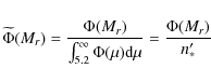
3 Stellar correlation function
3.1 Estimation of the correlation function
The angular two-point auto-correlation function (2PCF) ![]() is defined via the joint probability
is defined via the joint probability
![]() of finding objects in both the solid angles
of finding objects in both the solid angles
![]() and
and
![]()
where n is the mean density of objects in the sky and
where
Solving for w in Eq. (3) yields a simple estimator for the 2PCF:
where
The 2PCF estimate
Another statistical measure equivalent to the 2PCF, which we use for visualising the data, is the
cumulative difference distribution (CDD)
![]() ,
giving the cumulative number of pairs in excess of a random distribution:
,
giving the cumulative number of pairs in excess of a random distribution:
with
3.2 Boundary effects
Stars close to the sample's boundary have a somewhat truncated ring
![]() and consequently show a lack of neighbours. However, as in the present
study the probed angular scale is small compared to the sample's size,
it turns out that these edge effects have a negligible impact on
our results: we estimate the relative error introduced in
and consequently show a lack of neighbours. However, as in the present
study the probed angular scale is small compared to the sample's size,
it turns out that these edge effects have a negligible impact on
our results: we estimate the relative error introduced in
![]() by omitting the edge correction to be less than
by omitting the edge correction to be less than
![]() for any given
for any given
![]() .
.
The stars near the boundary of a hole or a bright star mask
(in the following simply ``hole'') show a lack of neighbours, too.
Therefore, only a fraction
![]() of all pairs separated by an angular distance
of all pairs separated by an angular distance ![]() has been observed, and we need to correct the observed number of pairs
has been observed, and we need to correct the observed number of pairs ![]() .
The ``true'' number of pairs, corrected for edge effects, then reads as
.
The ``true'' number of pairs, corrected for edge effects, then reads as
|
(8) |
In calculating the fraction
|
(9) |
For smaller angular separations, the effect is even less.
Taking into consideration these edge effects, we rewrite the 2PCF estimate
and the CDD
3.3 Uncertainty of the correlation function estimate
As the values of
![]() at different separations are not independent, Poisson errors may underestimate the uncertainty in
at different separations are not independent, Poisson errors may underestimate the uncertainty in
![]() ,
especially when the angular scales under consideration are large (Hamilton 1993; Bernstein 1994). However, as we see in Sect. 5, the clustering of wide binary stars occurs on small angular scales (
,
especially when the angular scales under consideration are large (Hamilton 1993; Bernstein 1994). However, as we see in Sect. 5, the clustering of wide binary stars occurs on small angular scales (
![]() )
compared to the size of our sample (20 deg
)
compared to the size of our sample (20 deg ![]() 40 deg).
We therefore expect that using Poisson errors only underestimates the
true errors by a small amount in our case. Thus, we adopt Poissonian
errors on
40 deg).
We therefore expect that using Poisson errors only underestimates the
true errors by a small amount in our case. Thus, we adopt Poissonian
errors on ![]() :
:
Using Eq. (10) and Gauss' error propagation formula, we may write the uncertainty of the CF estimate
where we omitted the dependencies on
The uncertainty in the CDD
![]() is easily obtained in the same way:
is easily obtained in the same way:
3.4 Testing the procedure for a random sample
![\begin{figure}
\par\includegraphics[width=8.8cm,clip]{13109f03.eps}
\end{figure}](/articles/aa/full_html/2010/01/aa13109-09/img74.png)
|
Figure 3: 2PCF as inferred from a random sample (solid circles, left ordinate) and the corresponding CDD (open circles, right ordinate). Poisson errors are indicated as vertical lines. |
| Open with DEXTER | |
To test the validity of the procedure to estimate the 2PCF described in the previous sections, we generated a random sample having the same number of ``stars'' and distributed over the same area as the stars in our final sample. In addition, we made certain that the random sample contains the same number of holes with appropriate radii.
For the analysis of the random sample we wrote a dedicated computer program that lays a grid with a mesh size of 1 arcmin over the sample before counting the pairs. This grid acts as a distance filter and avoids calculating the distances between all possible pairs: only pairs with both their components within a cell or with them in two adjacent cells, respectively, were taken into account.
If our procedure is correct we would expect a zero signal in
both the 2PCF and the CDD when analysing a sample of randomly
distributed stars. Figure 3
shows the result of the analysis of our random sample. There is indeed
no clustering signal evident, neither in the 2PCF nor in the CDD.
The results are consistent throughout with a zero signal out to the
separation limit of 30
![]() (compare also with Fig. 5). This shows that our procedure for estimating the 2PCF is reliable.
(compare also with Fig. 5). This shows that our procedure for estimating the 2PCF is reliable.
4 The model
Our approach to modelling the angular 2PCF is based on a technique developed by Wasserman & Weinberg (1987), hereafter WW87. As we describe in more detail in the following sections, this technique makes some simple assumptions on the basic statistical properties of wide binaries, and projects these theoretical distributions on the observational plane using the selection criteria of a given (binary) star catalogue and the geometry of the Milky Way galaxy (see also Weinberg 1988).
Their long periods make it virtually impossible to distinguish wide binary stars from mere chance projections (optical pairs) by their orbital motion. Therefore, we do not attempt to identify individual wide binaries, but we look for a statistical signal stemming from physical wide pairs in the sample, solely exploiting precise stellar position measurements provided by the SDSS.
The original Wasserman & Weinberg (WW) technique calculates the projected separation distribution to compare it with a sample of wide binaries of known distance and angular separation. In the present study we are only dealing nwith angular separations. The calculation of wide binary counts as a function of angular separation alone requires an appropiate modification of the WW-technique (see also Garnavich 1991), which we discuss in Sect. 4.3.
4.1 Wasserman-Weinberg technique
WW87 developed ``a versatile technique for comparing wide binary
observations with theoretical semimajor axis distributions''. According
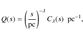
to WW87 we may write the number of observed binaries
![]() with projected physical separations between s and
with projected physical separations between s and
![]() in a given catalogue of stars as
in a given catalogue of stars as
where
The total number density
![]() is
one of the two free parameters in the model that will be inferred by
fitting the model to the observational data. The reduced separation
distribution Q(s)
contains the physical properties from the wide binaries (semi-major
axis distribution, distribution of eccentricities, orientation of the
orbital planes) projected onto the observational plane, whereas the
effective volume V(s) takes into
account the characteristics of the sample under consideration (covered
area, range of angular separation examined, magnitude limits), as well
as the stellar density distribution in the Galaxy and the luminosity
function.
is
one of the two free parameters in the model that will be inferred by
fitting the model to the observational data. The reduced separation
distribution Q(s)
contains the physical properties from the wide binaries (semi-major
axis distribution, distribution of eccentricities, orientation of the
orbital planes) projected onto the observational plane, whereas the
effective volume V(s) takes into
account the characteristics of the sample under consideration (covered
area, range of angular separation examined, magnitude limits), as well
as the stellar density distribution in the Galaxy and the luminosity
function.
As we show in Sect. 4.3, this neat formal splitting in physical properties and selection effects will not be possible anymore after the required modification on the WW-technique mentioned above. At this point, we discuss the two parts - Q(s) and V(s) - more in detail.
4.1.1 Reduced separation distribution
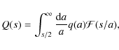
The reduced separation distribution Q(s) is given by the projection of the reduced (present-day) semi-major axis distribution q(a)
against the sky. Gravitational perturbations due to stars, giant
molecular clouds, and (hypothetical) DM particles cause the
semi-major axes of (disc) wide binaries to evolve. Little is known
about the initial semi-major axis distribution, and usually a single
power-law is assumed, because of its simplicity (Weinberg 1988) but also because of theoretical considerations (Poveda et al. 2007; Valtonen 1997, and references therein). The evolution of the semi-major axis distribution of disc wide binaries has been modelled by Weinberg et al. (1987)
in terms of the Fokker-Plack equation. Their numerical simulations
suggest that the semi-major axis distribution evolves in a self-similar
way for reasonable choices of the initial power-law index and the wide
binary birth rate function. We decided, therefore, to model the
present-epoch semi-major axis distribution of wide binary stars q(a) by a single powerlaw
with the power-law index
We normalise q(a) - hence the name ``reduced semi-major axis distribution'' - such that
|
(17) |
giving
|
(18) |
where
![\begin{displaymath}%
c_\lambda=\left\{\begin{array}{ll} (1-\lambda)\left[a_{\rm ...
...{\min}\right]^{-1}, & \mbox{for } \lambda=1\end{array}\right.
\end{displaymath}](/articles/aa/full_html/2010/01/aa13109-09/img87.png)
|
(19) |
with
In a more general treatment, q(a) might also depend on the luminosity classes of the binary star members, as well as on their magnitudes. Like WW87, we restrict our analysis to models where q(a) only depends on the semi-major axis a.
It is somewhat disputed whether the semi-major axis distribution has a break at larger a attributed to the disruptive effects of the environment on the widest binary stars. In their extensive work Wasserman & Weinberg (1991) (see also Weinberg 1990) conclud that ``although the data suggest a break in the physical distribution of wide binary separations, they do not require a break with overwhelming statistical significance'', whereas the more recent study by Lépine & Bongiorno (2007) shows evidence for a break at ![]() AU (statistically, we have
AU (statistically, we have
![]() ;
see Eq. (22)). In this context, the question arises whether the assumption that the data is described by a single powerlaw (Eq. (16)) up to the tidal limit
;
see Eq. (22)). In this context, the question arises whether the assumption that the data is described by a single powerlaw (Eq. (16)) up to the tidal limit ![]() can be rejected with confidence. We address this question in Sect. 5.
can be rejected with confidence. We address this question in Sect. 5.
Assuming that ``the binaries' orbital planes are randomly oriented and that their eccentricities e are distributed uniformly in e2'' (WW87) we can project q(a) against the sky by (Weinberg 1988)
where
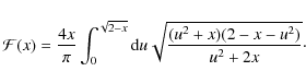
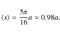
With the above assumptions on the orientations of the orbital planes and the distribution of eccentricities it can be shown that the average observed projected separation
From the normalisations of q(a) it also follows that Q(s) is normalised to unity in the range
Substituting
![]() in Eq. (20), as well as
in Eq. (20), as well as
![]() in Eq. (21)
leads to a convenient form for numerical integration
in Eq. (21)
leads to a convenient form for numerical integration
|
(23) |
where
The integrals in Eq. (24) are evaluated using Gauss quadrature (Press et al. 1992). For s far from
|
(25) |
4.1.2 Effective volume
As we deal with a magnitude-limited sample, we are plagued by selection
effects that must be properly taken into account. Following WW87, we do
this by means of the effective volume. It allows for the solid angle ![]() covered by the sample, the angular separation range
covered by the sample, the angular separation range
![]() we are examining, and the apparent magnitude limits
we are examining, and the apparent magnitude limits ![]() and
and ![]() .
Furthermore, the effective volume takes the stellar density distribution
.
Furthermore, the effective volume takes the stellar density distribution ![]() into account, as well as the normalised (single star) luminosity function
into account, as well as the normalised (single star) luminosity function
![]() (both described more in detail in Sect. 4.2).
(both described more in detail in Sect. 4.2).
``Making the plausible assumptions that the intrinsic luminosities of
the two stars in a wide binary are independent and distributed in the
same way as the luminosities of field stars'' (WW87), and assuming
further that the stellar density distribution ![]() is independent of the stars' absolute luminosities, we may write the effective volume as
is independent of the stars' absolute luminosities, we may write the effective volume as
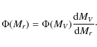
where we have the standard relations
and
![\begin{figure}
\par\includegraphics[width=8.8cm,clip]{13109f04.eps}
\end{figure}](/articles/aa/full_html/2010/01/aa13109-09/img111.png)
|
Figure 4: Effective volumes calculated using the parameters that correspond to our final sample (Table 2) for the three Galactic structure parameter sets as discussed in Sect. 4.2. Long dashed line: set 1; solid line: set 2; short dashed line: set 3. |
| Open with DEXTER | |
In Fig. 4 the
effective volumes for the three Galactic structure parameter sets
(described in the next section) are plotted using the parameters that
correspond to our final sample (see Table 2). From the effective volume V(s), it is evident that our study is most sensitive to projected separations in
![]() pc, whereas our study is absolutely insensitive when
pc, whereas our study is absolutely insensitive when
![]() pc or
pc or ![]() pc. Referring to Eq. (22), we see that the shape of the effective volume also indicates that we are insensitive to semi-major axis
pc. Referring to Eq. (22), we see that the shape of the effective volume also indicates that we are insensitive to semi-major axis
![]() pc and for
pc and for ![]() pc, which nicely fits the range in a
where we assume that the single power-law model holds. But it also
shows that our analysis is not too sensitive to very wide binary stars
with semi-major axes larger than 0.1 pc.
pc, which nicely fits the range in a
where we assume that the single power-law model holds. But it also
shows that our analysis is not too sensitive to very wide binary stars
with semi-major axes larger than 0.1 pc.
4.2 Galactic model
4.2.1 Stellar density distribution
Following earlier work (especially Chen et al. 2001; Juric et al. 2008, and references therein), we modelled the stellar density distribution of the Milky Way Galaxy by including two exponential disc components - a thin and a thick disc - and an elliptical halo component whose density profile obeys a powerlaw. The contribution of the Galactic bulge is negligible in the direction of the NGP and it is therefore ignored in the following.
The three components are added to yield the total density distribution
| (29) |
with
|
(30) |
which is normalised such that
Both the thin and the thick disc populations obey a double exponential density law of the form (e.g. Bahcall & Soneira 1980)
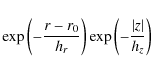
where hr and hz are the scale length and the scale height of the disc, z is the object's height above the Galactic midplane, and r is its Galactocentric distance in the Galactic plane. We take the Sun's distance from the centre of the Galaxy in the Galactic plane to be r0=8 kpc. Juric et al. (2008) find that the Sun is located
| (32) | ||
| (33) | ||
| (34) |
where d is its distance from the Sun in the Galactic plane and
In line with Juric et al. (2008) and Chen et al. (2001) we assume the scale heights to be independent of absolute magnitude M.
Using capitals for the thick disc's and lower case letters for the thin
disc's scale height and length, we may write the normalised number
density distribution of the stars in the Galactic thin disc as
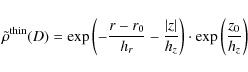
|
(35) |
and that of the thick disc as
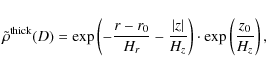
|
(36) |
where the rightmost factors are for normalisation purposes and ensure that
The density distribution of the stellar halo population is modelled by a powerlaw with index k.
The observational data prefer a somewhat oblate halo giving an
ellipsoid, flattened in the same sense as the Galactic disc, with axes a=b and
![]() ,
where
,
where ![]() controls the ellipticity of the halo (cf. Juric et al. 2008)
controls the ellipticity of the halo (cf. Juric et al. 2008)
![\begin{displaymath}%
\tilde\rho^{\rm halo}(D)=\left[\frac{r^2+\left(\frac{z}{\ka...
..._0^2+\left(\frac{z_0}{\kappa}\right)^2}\right]^{-\frac{k}{2}},
\end{displaymath}](/articles/aa/full_html/2010/01/aa13109-09/img136.png)
which, of course, also satisfies
We compare three different sets of structure parameters:
- Set 1:
- the measured values from Juric et al. (2008) (see their Table 10). These values are best-fit parameters as directly measured from the apparent number density distribution maps using their ``bright'' photometric parallax relation (their Eq. (2)). They are not corrected for bias caused by, e.g., unresolved stellar multiplicity, hence the term ``apparent''.
- Set 2:
- the bias-corrected values from Juric et al. (2008) (see again their Table 10). These values were corrected for unrecognised stellar multiplicity, Malmquist bias, and systematic distance determination errors by means of Monte Carlo-generated mock catalogues (Juric et al. 2008, Sect. 4.3.). Following Reid & Gizis (1997), the fraction of ``stars'' in the local stellar population that in fact are unresolved binaries is taken to be 35%. However, the halo component was not included in the mock catalogues, and its structure parameters were therefore not corrected, but the measured values are used instead. This set of parameters will be referred to as our standard set.
- Set 3:
- as a third independent set of Galactic structure parameters, we refer to the somewhat earlier work of Chen et al. (2001). It is also based on observations obtained with the SDSS, but Chen et al. (2001) infer the density distribution of the stars by inverting the fundamental equation of stellar statistics (e.g. Karttunen et al. 1996).
Table 1: Galactic structure parameters.
4.2.2 Stellar luminosity function
For our study we refer to the luminosity function (LF) inferred by Jahreiß & Wielen (1997) using Hipparcos parallaxes, which gives reliable values for a wide magnitude range (
![]() ). (The faint end of the LF is somewhat uncertain and Jahreiß & Wielen 1997, give only a lower limit in the range
). (The faint end of the LF is somewhat uncertain and Jahreiß & Wielen 1997, give only a lower limit in the range
![]() .
We take that lower limit at the faint end to be the true value of the LF in that magnitude range.)
.
We take that lower limit at the faint end to be the true value of the LF in that magnitude range.)
Table 2: Parameters of the final sample and of the subsamples.
We need to transform the Jahreiß & Wielen (1997) LF from visual (V-band) into r-band magnitudes, i.e. from ![]() to
to ![]() .
We perform this transformation in an unsophisticated way by combining the photometric parallax relation from Laird et al. (1988), which was calibrated using the Hyades and is linear in (B-V) (their Eq. (1a))
.
We perform this transformation in an unsophisticated way by combining the photometric parallax relation from Laird et al. (1988), which was calibrated using the Hyades and is linear in (B-V) (their Eq. (1a))
| (38) |
with a transformation equation that is obtained by subtracting Eqs. (1) from (3) in Bilir et al. (2005)
| (39) |
The linearity of the photometric parallax relation removes any inversion problem, since it assures - in a mathematical sense - that a colour index (B-V) exists for every MV. For a given distance we then have
| (40) |
and the transformed LF is simply
|
(41) |
Using linear interpolation (the brightest bin at Mr=-1 mag is an extrapolation), we finally have rebinned
We normalise the LF by integrating over the absolute magnitude range corresponding to our total sample
|
(42) |
with
4.3 Modification of the Wasserman-Weinberg technique
To derive a theoretical angular 2PCF we need to calculate the expected number of wide binaries as a function of angular separation. To this end, the above-described WW-technique requires the modification that we address now.
Let
![]() be the number of wide binaries observed with an angular separation between
be the number of wide binaries observed with an angular separation between ![]() and
and
![]() .
For a given distance D, we have
.
For a given distance D, we have
![]() and
and ![]() .
(Note that our unit for s and D is pc, whereas
.
(Note that our unit for s and D is pc, whereas ![]() is in rad.) The latter expression can be used to write the reduced separation distribution Q(s) as
is in rad.) The latter expression can be used to write the reduced separation distribution Q(s) as
![]() .
This introduces an explicit dependency on D, so we need to incorporate
.
This introduces an explicit dependency on D, so we need to incorporate
![]() into the integration over D in the formula for the effective volume (Eq. (26)).
This incorporation is the reason it is no longer possible to separate
the reduced separation distribution from the effective volume in a
formal way like in Eq. (15).
into the integration over D in the formula for the effective volume (Eq. (26)).
This incorporation is the reason it is no longer possible to separate
the reduced separation distribution from the effective volume in a
formal way like in Eq. (15).
Furthermore, we need to modify the limits in the integration over D in Eq. (15). Recalling that for a given semi-major axis a, the average observed projected separation is
![]() (Eq. (22)), it appears to be appropriate to let the integration limits run from
(Eq. (22)), it appears to be appropriate to let the integration limits run from
![]() to
to
![]() (Garnavich 1991). We take
(Garnavich 1991). We take
![]()
![]() 10-4 pc and
10-4 pc and
![]() (for the calculation of the tidal limit
(for the calculation of the tidal limit ![]() see Appendix B).
see Appendix B).
Putting it all together, we may write the number of observed wide binaries as a function of
angular separation as
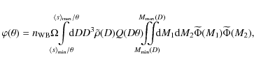
where we have included an additional factor D into the integration over D, because
The model-2PCF is now determined by adding the number of physical pairs, calculated by Eq. (43), to the number of pairs expected from a random sample given by Eq. (6)
The two free parameters -
4.4 Fitting procedure
We determine the two free parameters of the model,
![]() and
and ![]() ,
by means of a Levenberg-Marquardt nonlinear least-square algorithm (Lourakis 2004)
,
by means of a Levenberg-Marquardt nonlinear least-square algorithm (Lourakis 2004)![]() , which minimises the value of the
, which minimises the value of the ![]() defined as
defined as
The data is binned in steps of
Following Press et al. (1992), we use the incomplete gamma function
![]() with
with
![]() degrees of freedom as a quantitative measure of the goodness-of-fit. (N-2 because the model has two free parameters:
degrees of freedom as a quantitative measure of the goodness-of-fit. (N-2 because the model has two free parameters:
![]() and
and ![]() .) Values of Q near unity indicate that the model adequately represents the data.
.) Values of Q near unity indicate that the model adequately represents the data.
4.5 Confidence intervals
To estimate the uncertainties of our best-fit values, we use Monte Carlo confidence intervals (MCCRs) (e.g. Press et al. 1992, Sect. 15.6). Assuming Poissonian errors, we generate 10 000 synthetic data sets by drawing the number of unique pairs ``observed'' in the kth synthetic sample
![]() from a Poisson distribution with mean
from a Poisson distribution with mean ![]() ,
where
,
where ![]() is the observed number of pairs, not
corrected for edge effects due to survey holes. The ``true'' number of
pairs in a synthetic sample is then given by dividing
is the observed number of pairs, not
corrected for edge effects due to survey holes. The ``true'' number of
pairs in a synthetic sample is then given by dividing
![]() by
by
![]() (see Sect. 3.2).
(see Sect. 3.2).
For each synthetic sample, we determine best-fit values for the model's free parameters,
![]() and
and
![]() ,
in a least-square sense as described above. A
,
in a least-square sense as described above. A ![]() -MCCR is defined by the line of constant
-MCCR is defined by the line of constant ![]() which encloses
which encloses ![]() of the best-fit values in the
of the best-fit values in the
![]() versus
versus ![]() plane (see Fig. 6). The confidence intervals of
plane (see Fig. 6). The confidence intervals of
![]() and
and ![]() are then given by the orthogonal projection of the MCCR onto the corresponding axis.
are then given by the orthogonal projection of the MCCR onto the corresponding axis.
We include in our error estimate only the uncertainties stemming from the pair counts in ![]() .
Neither the uncertainties in the Galactic structure parameters nor those in the LF are taken into account.
.
Neither the uncertainties in the Galactic structure parameters nor those in the LF are taken into account.
5 Results
5.1 Analysis of the total sample
The results of the analysis for the total sample are shown in Fig. 5 and Table 3. Figure 5 shows the 2PCF estimate
![]() and the CDD
and the CDD
![]() .
The statistical uncertainties calculated according to Eq. (13) are shown as vertical lines. A strong clustering signal out to at least
.
The statistical uncertainties calculated according to Eq. (13) are shown as vertical lines. A strong clustering signal out to at least
![]() is
evident, whereas the CDD suggest that there are pairs in excess of a
random distribution up to maximum angular separation examined, that is,
up to 30
is
evident, whereas the CDD suggest that there are pairs in excess of a
random distribution up to maximum angular separation examined, that is,
up to 30
![]() .
The outlier at
.
The outlier at
![]() is probably a random fluctuation. We also plot in Fig. 5 best-fitting models using the three Galactic structure parameter sets described in Sect. 4.2.1.
is probably a random fluctuation. We also plot in Fig. 5 best-fitting models using the three Galactic structure parameter sets described in Sect. 4.2.1.
The best-fit values of the two free parameters,
![]() and
and ![]() ,
are tabulated in Table 3 for the three Galactic structure parameter sets. The power-law index
,
are tabulated in Table 3 for the three Galactic structure parameter sets. The power-law index ![]() appears to be quite independent of the set we choose. The wide binary density
appears to be quite independent of the set we choose. The wide binary density
![]() ,
on the other hand, shows some variation. The difference between
the sets 1 and 2 reflects, for the most part, the difference
in the overall normalisation
,
on the other hand, shows some variation. The difference between
the sets 1 and 2 reflects, for the most part, the difference
in the overall normalisation ![]() of the density distribution, whereas in set 3 the unequal halo
normalisation with respect to the other two sets also contributes to
the difference in
of the density distribution, whereas in set 3 the unequal halo
normalisation with respect to the other two sets also contributes to
the difference in
![]() .
.
We also list the goodness-of-fit Q and the corresponding reduced chi-square values (![]() divided by the degrees of freedom
divided by the degrees of freedom ![]() )
in Table 3.
All three sets of Galactic structure parameters give equally good fits,
whereas the reduced chi-square values, which are only slightly more
than unity, indicate that we have not severely underestimated the
uncertainty in the 2PCF.
)
in Table 3.
All three sets of Galactic structure parameters give equally good fits,
whereas the reduced chi-square values, which are only slightly more
than unity, indicate that we have not severely underestimated the
uncertainty in the 2PCF.
![\begin{figure}
\par\includegraphics[width=8.8cm,clip]{13109f05.eps}
\end{figure}](/articles/aa/full_html/2010/01/aa13109-09/img179.png)
|
Figure 5: 2PCF as inferred from the total sample (solid circles, left ordinate) and the corresponding CDD (open circles, right ordinate). Poisson errors are indicated as vertical lines. Model curves for the three Galactic structure parameter sets are plotted, too, but as the differences between them are marginal they lie one upon the other, giving a single solid line. |
| Open with DEXTER | |
Table 3: Best-fit values: total sample.
![\begin{figure}
\par\includegraphics[width=8.8cm,clip]{13109f06.eps}
\end{figure}](/articles/aa/full_html/2010/01/aa13109-09/img182.png)
|
Figure 6:
Distribution of the best-fit values for the total sample using the
structure parameter set 2 obtained by the Monte Carlo
procedure described in the text. The solid contours (MCCRs) are lines
of constant |
| Open with DEXTER | |
![\begin{figure}
\par\includegraphics[width=8.8cm,clip]{13109f07.eps}
\end{figure}](/articles/aa/full_html/2010/01/aa13109-09/img183.png)
|
Figure 7:
MCCRs for the three Galactic structure parameter sets corresponding to
the total sample. Long dashed line: set 1; solid line: set 2;
short dashed line: set 3. The crosses indicate the best-fit values
inferred from the true observed number of pairs,
|
| Open with DEXTER | |
In Fig. 6 we
show, representative of the other structure parameter sets, the
distribution of the best-fit values from the synthetic samples using
set 2, our standard set. In the same figure the 68.3% (![]() ), 95.4% (
), 95.4% (![]() ), and 99.7% (
), and 99.7% (![]() )
MCCRs are also plotted. Quoting 95.4% confidence intervals
throughout, we find for our final sample using the Galactic structure
parameter set 2
)
MCCRs are also plotted. Quoting 95.4% confidence intervals
throughout, we find for our final sample using the Galactic structure
parameter set 2
|
(46) |
The power-law index
|
(47) |
where
We show the confidence regions corresponding to the three sets of Galactic structure parameters in Fig. 7. The confidence intervals for ![]() agree for all the sets,
which demonstrates that we can determine
agree for all the sets,
which demonstrates that we can determine ![]() and
its confidence intervals reliably - provided that no systematic
error has crept into our analysis. The wide binary density
and
its confidence intervals reliably - provided that no systematic
error has crept into our analysis. The wide binary density
![]() ,
on the other hand, is more sensitive to the exact values of the Galactic structure parameters than
,
on the other hand, is more sensitive to the exact values of the Galactic structure parameters than ![]() is, so the values we have derived for the wide binary density
is, so the values we have derived for the wide binary density
![]() and the fraction
and the fraction
![]() should be viewed with caution. We are, however, confident that the true value of the wide binary density
should be viewed with caution. We are, however, confident that the true value of the wide binary density
![]() is within a factor of 2 of our derived value.
is within a factor of 2 of our derived value.
Since the structure parameter set 2 is - as far as known to the authors - the only one systematically corrected for unresolved multiplicity, we give that set more weight. From now on, we use the bias-corrected values from Juric et al. (2008), i.e. our standard set 2, exclusively.
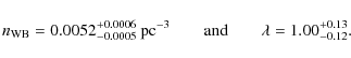
Having determined the two free parameter in our model, we can calculate the number of wide binaries in our total sample as a function of the projected separation s. We show the distribution in Fig. 8 whose shape is largely dominated by the effective volume, i.e. by selection effects. In particular, this distribution implies that we have observed 830+250-215 very wide binaries with a projected separation larger than 0.1 pc in our total sample, while none are expected to be found beyond 0.8 pc, given our selection criteria. However, that extremely wide binaries with projected separations of more than 1 pc can exist in the Galactic halo has recently been confirmed by Quinn et al. (2009).
![\begin{figure}
\par\includegraphics[width=8.8cm,clip]{13109f08.eps}
\vspace*{3mm}
\end{figure}](/articles/aa/full_html/2010/01/aa13109-09/img190.png)
|
Figure 8: Distribution of wide binaries as a function of projected separation s that is expected to be observed in the total sample, given the model assumptions and the selection criteria we have adopted (see text). |
| Open with DEXTER | |
5.2 Differentiation in terms of apparent magnitude
![\begin{figure}
\par\includegraphics[width=8.8cm,clip]{13109f09.eps}
\end{figure}](/articles/aa/full_html/2010/01/aa13109-09/img191.png)
|
Figure 9:
2PCF and CDD for the r<20.0 mag and r<19.5 mag
subsamples together with the corresponding model curves. Up-pointing
triangles (long-dashed lines) are for the r<20.0 mag subsample, whereas down-pointing triangles (short-dashed lines) are for the r<19.5 mag subsample. The symbols were shifted apart by
|
| Open with DEXTER | |
![\begin{figure}
\par\includegraphics[width=8.8cm,clip]{13109f10.eps}
\end{figure}](/articles/aa/full_html/2010/01/aa13109-09/img192.png)
|
Figure 10: MCCRs for the r<20.0 mag (long dashed contours) and r<19.5 mag (short-dashed contours) subsamples. For comparison, the MCCR for our final sample is also shown (solid-contours). The crosses have the same meaning as in Fig. 7. |
| Open with DEXTER | |
To test the consistency of the standard model, we used two subsamples having brighter upper apparent magnitude limits than our total sample and analysed them in the same way as the total sample itself. We set the upper apparent magnitude limit to r=20.0 mag and r=19.5 mag - all other selection criteria (including the lower apparent magnitude limits) remain unchanged. The main parameters of these subsamples are listed in Table 2.
Table 4: Best-fit values: r<20.0 mag and r<19.5 mag.
In Fig. 9 we show the 2PCF and the CCD as in Fig. 5, together with the corresponding model curves for standard set 2 (see caption). The best-fit values are listed in Table 4. The MCCRs of the r<20.0 mag and r<19.5 mag subsamples are shown in Fig. 10.
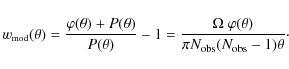
If the model were self-consistent, we would expect that the best-fit values agree with each other within their uncertainties. Figure 10 indicates that this is not the case: It appears that the best-fit values are systematically shifted to higher densities and larger power-law indices when using a brighter upper magnitude limit. As we discuss in Sect. 6.2, this inconsistency is most likely an artefact of the (oversimplifying) model assumptions and does not entirely undermine our results.
5.3 Differentiation in terms of direction
![\begin{figure}
\par\includegraphics[width=8.8cm,clip]{13109f11.eps}
\end{figure}](/articles/aa/full_html/2010/01/aa13109-09/img193.png)
|
Figure 11: 2PCF and CDD for the
left and the right subsamples, together with the corresponding model
curves. Left-pointing triangles (long-dashed lines) are for the left
subsample, whereas right-pointing triangles (short-dashed lines) are
for the right subsample. The symbols were shifted apart by
|
| Open with DEXTER | |
![\begin{figure}
\par\includegraphics[width=8.8cm,clip]{13109f12.eps}
\end{figure}](/articles/aa/full_html/2010/01/aa13109-09/img194.png)
|
Figure 12: MCCRs for the left (long-dashed contours) and right (short-dashed contours) subsamples. For comparison, also the MCCR for our final sample is shown (solid contours). The crosses have the same meaning as in Fig. 7. |
| Open with DEXTER | |
Table 5: Best-fit values: left and right.
![\begin{figure}
\par\includegraphics[width=18cm,clip]{13109f13.eps}
\end{figure}](/articles/aa/full_html/2010/01/aa13109-09/img195.png)
|
Figure 13: 2PCF (solid circles) and CDD (open circles) for the subsamples A to H, together with the corresponding model curves. The subfigures are arranged as the corresponding subareas would be seen on the sky. |
| Open with DEXTER | |
In a previous study, Saarinen & Gilmore (1989) found that the binaries appear to be highly clumped in the NGP. However, it has not become entirely clear whether this patchiness of the wide binary distribution in the sky is a real physical characteristic of the wide binary population or if it is due to statistical fluctuations. In principle, we can check whether the wide binary density varies with position in the sky by dividing our sample into subareas.
To begin with, we divide our sample in two halves by cutting it along the
![]() meridian. In the following, we refer to the subarea with
meridian. In the following, we refer to the subarea with
![]() as
the ``left'' subsample and the other half as the ``right'' subsample.
The subsamples' main parameters are listed in Table 2.
as
the ``left'' subsample and the other half as the ``right'' subsample.
The subsamples' main parameters are listed in Table 2.
In Fig. 11 we show the 2PCFs inferred from the left and the right sample, as well as the corresponding CDDs. It appears that there are a few more pairs in excess of random in the left half. In the same figure also the corresponding model curves are plotted. The best-fit values are listed in Table 5.
In Fig. 12 we
show the MCCRs of the left and the right subsamples. The left subsample
indeed shows a higher wide binary density than the right one. The
difference is significant at the ![]() level.
The power-law indices, on the other hand, do agree in both subsamples.
Regarding the total sample, the right half differs significantly
(at
level.
The power-law indices, on the other hand, do agree in both subsamples.
Regarding the total sample, the right half differs significantly
(at ![]() ), whereas the left half is more consistent with it.
), whereas the left half is more consistent with it.
The difference in the wide binary density between the left and the
right halves is probably a real feature, as any inadequacies of our
model (e.g. inaccuracies of the stellar density distribution
we use) should affect both halves in almost the same manner.
To examine this apparent positional dependency of the wide binary
density in more detail, we divide our sample further into eight
subsamples, each covering
![]()
![]()
![]() .
They are labelled from A (``upper left'') to H (``lower right'') as suggested in Fig. 13, where the abscissa can thought of representing the right ascension from
.
They are labelled from A (``upper left'') to H (``lower right'') as suggested in Fig. 13, where the abscissa can thought of representing the right ascension from
![]() (``left'') to
(``left'') to
![]() (``right'') and similarly the ordinate represents the declination from
(``right'') and similarly the ordinate represents the declination from
![]() (``bottom'') to
(``bottom'') to
![]() (``top''). The subsample's main parameters are again summarised in Table 2.
(``top''). The subsample's main parameters are again summarised in Table 2.
Table 6: Best-fit values: A to H.
Figure 13 shows the 2PCFs
estimate and the CDDs with the best-fit model curves. The corresponding
best-fit parameters are listed in Table 6.
Some subtle differences are apparent between different subsamples.
While the CDD in A-C, and G are reproduced well by the model,
the CDD in D, F, and H appears to be too flat. In those
subsamples it seems that almost no physical pairs are present at
angular separations over
![]() ,
in agreement with the findings of Sesar et al. (2008) (see Sect. 6.1).
,
in agreement with the findings of Sesar et al. (2008) (see Sect. 6.1).
The subsample E appears to be an outlier, because it contains almost twice as many pairs in excess of random as the seven other subsamples. The listed best-fit values confirm the peculiar character of subsample E having the highest wide binary density of all eight subsamples, together with the lowest power-law index. As far as the authors can judge, there is no obvious special feature (e.g. open star cluster) in subsample E that could cause this anomaly.
![\begin{figure}
\par\includegraphics[width=8.8cm,clip]{13109f14.eps}
\end{figure}](/articles/aa/full_html/2010/01/aa13109-09/img205.png)
|
Figure 14: 95.4% MCCRs for the subsamples A to H. The crosses have the same meaning as in Fig. 7. |
| Open with DEXTER | |
The ![]() MCCR are shown in Fig. 14.
Except for the outlier E, all the other subsamples are quite
consistent with each other. Also, no obvious trend, e.g. with
Galactic latitude b, is apparent. To what extent is the subsample E responsible for the difference between the right and the left subsamples?
MCCR are shown in Fig. 14.
Except for the outlier E, all the other subsamples are quite
consistent with each other. Also, no obvious trend, e.g. with
Galactic latitude b, is apparent. To what extent is the subsample E responsible for the difference between the right and the left subsamples?
To answer this question, we repeated the analysis of the total and left
(sub)sample excluding subsample E. The results are listed in
Table 7.
The wide binary density drops significantly to a value more consistent
with the right subsample. Thus, we conclude that the difference between
the right and the left subsamples is largely caused by the
outlier E. Apart from subsample E, the wide binary densities
in different directions appear to be consistent with each other. The
reason for the high density in subsample E remains unclear.
However, a statistical fluctuation cannot be ruled out to a level
better than ![]() .
.
6 Discussion
Table 7: Best-fit values: excluding subsample E.
![\begin{figure}
\par\includegraphics[width=8.8cm,clip]{13109f15.eps}
\end{figure}](/articles/aa/full_html/2010/01/aa13109-09/img206.png)
|
Figure 15: 2PCF and CDD as inferred from our total sample as in Fig. 5. The model curve is for the broken power-law model from Lépine & Bongiorno (2007) (see text). |
| Open with DEXTER | |
6.1 External (in)consistencies
In this section we compare our results with those of previous studies. Our first point concerns the observed angular 2PCF. From the CDD of our total sample shown in Fig. 5 we have noted pairs in excess of random up to
![]() .
This is contradictory to Sesar et al. (2008) who find that there are essentially no physically bound pairs with an angular separation
.
This is contradictory to Sesar et al. (2008) who find that there are essentially no physically bound pairs with an angular separation
![]() .
(We note, however, that this is in accord with some of our subsamples, see Fig. 13.) We considered several possible reasons for this apparent discrepancy, such as differences in the selection criteria of the Sesar et al.
sample with respect to our sample, underestimation of the total area of
holes in our sample, or an overcorrection of edge effects due to
those holes, but we convinced ourselves that none of them can account
for this disagreement. A real physical difference in the wide
binary population studied, e.g. caused by the fact that Sesar et al.'s sample is largely disc-dominated, while our final sample has a substantial halo contribution of
.
(We note, however, that this is in accord with some of our subsamples, see Fig. 13.) We considered several possible reasons for this apparent discrepancy, such as differences in the selection criteria of the Sesar et al.
sample with respect to our sample, underestimation of the total area of
holes in our sample, or an overcorrection of edge effects due to
those holes, but we convinced ourselves that none of them can account
for this disagreement. A real physical difference in the wide
binary population studied, e.g. caused by the fact that Sesar et al.'s sample is largely disc-dominated, while our final sample has a substantial halo contribution of
![]() ,
can be excluded, as previous studies (Chanamé & Gould 2004; Latham et al. 2002) found that the disc and halo wide binary populations are reasonably consistent in their statistical characteristics.
,
can be excluded, as previous studies (Chanamé & Gould 2004; Latham et al. 2002) found that the disc and halo wide binary populations are reasonably consistent in their statistical characteristics.
Regarding the wide binary fraction, Sesar et al.
also find a much smaller wide binary fraction of below 1%
(decreasing with height above the Galactic plane), as compared to
our
![]()
![]() 10%. Even if all pairs with a semi-major axis larger than
3000 AU (beyond the ``break'') were ignored, we would still find a
wide binary fraction of 4.6%. On the other hand, Lépine & Bongiorno (2007)
give a binary fraction of at least 9.5% for separations larger
than 1000 AU, which is in rough agreement with our results
(setting
10%. Even if all pairs with a semi-major axis larger than
3000 AU (beyond the ``break'') were ignored, we would still find a
wide binary fraction of 4.6%. On the other hand, Lépine & Bongiorno (2007)
give a binary fraction of at least 9.5% for separations larger
than 1000 AU, which is in rough agreement with our results
(setting
![]() AU we find
AU we find
![]()
![]() 8.3%).
8.3%).
Studying a much smaller region containing brighter stars as compared to our sample, WW87 and Garnavich (1991,1988) found an unphysically large wide binary density in the direction of the NGP. Saarinen & Gilmore (1989) attribute this overdensity to a large statistical fluctuation. The region where this overdensity was found would be located in our subarea H. But as we probe fainter stars, no density enhancement is evident in that subarea. The slight overdensity we found in subarea E is different from that previously noted by WW87 and Garnavich.
As to the separation distribution, previous studies have found that the observational data are described by Öpik's law (![]() )
up to a certain maximum separation (``break''): Lépine & Bongiorno (2007) find this break to be around 3500 AU, beyond which a steeper slope, with
)
up to a certain maximum separation (``break''): Lépine & Bongiorno (2007) find this break to be around 3500 AU, beyond which a steeper slope, with
![]() ,
should apply. Sesar et al. (2008) basically agree with Lépine & Bongiorno and find in addition that the maximum separation increases with height above the Galactic plane. Poveda & Allen (2004) divided their wide binary catalogue (Poveda et al. 1994)
into two subsamples consisting of the oldest and youngest systems,
respectively, and find that the ``maximum major semiaxis for which Öpik's distribution holds is much larger for the youngest binaries (am=7862 AU) than for the oldest (am=2409 AU)''. Chanamé & Gould (2004)
find the data to be described by a single powerlaw with an index of
approximately 1.6 for their disc and halo samples. However, they
note a ``puzzling'' flattening of the distribution of the disc
binaries between 10
,
should apply. Sesar et al. (2008) basically agree with Lépine & Bongiorno and find in addition that the maximum separation increases with height above the Galactic plane. Poveda & Allen (2004) divided their wide binary catalogue (Poveda et al. 1994)
into two subsamples consisting of the oldest and youngest systems,
respectively, and find that the ``maximum major semiaxis for which Öpik's distribution holds is much larger for the youngest binaries (am=7862 AU) than for the oldest (am=2409 AU)''. Chanamé & Gould (2004)
find the data to be described by a single powerlaw with an index of
approximately 1.6 for their disc and halo samples. However, they
note a ``puzzling'' flattening of the distribution of the disc
binaries between 10
![]() and 25
and 25
![]() .
As already suggested by Sesar et al., this flat range might be the domain where Öpik's law is valid.
In view of the substantial uncertainties inherent in studies by Lépine & Bongiorno and by Chanamé & Gould, the two studies appear to be broadly consistent.
Similar to our study, Garnavich (1991) assumed that the semi-major axis distribution is described by a single powerlaw. He finds the power-law index to be 0.7
.
As already suggested by Sesar et al., this flat range might be the domain where Öpik's law is valid.
In view of the substantial uncertainties inherent in studies by Lépine & Bongiorno and by Chanamé & Gould, the two studies appear to be broadly consistent.
Similar to our study, Garnavich (1991) assumed that the semi-major axis distribution is described by a single powerlaw. He finds the power-law index to be 0.7 ![]() 0.2
for his NGP sample covering nearly 240 square degree. At
intermediate Galactic latitudes he finds the slope to be steeper:
0.2
for his NGP sample covering nearly 240 square degree. At
intermediate Galactic latitudes he finds the slope to be steeper:
![]()
![]() 0.2. His data seem to favour a (somewhat unrealistic
0.2. His data seem to favour a (somewhat unrealistic![]() ) ``cutoff'' around 0.1 pc, especially for the NGP sample.
) ``cutoff'' around 0.1 pc, especially for the NGP sample.
The question of a break in the separation distribution has much been discussed in the context of DM constraints. Wasserman & Weinberg (1991), for example, show that the observational data suggest a break but they do not require one statistically. Looking at the CDD for our total sample in Fig. 5,
we note that our best-fit model slightly overestimates the number of
pairs in excess of random at larger angular separations, and a more
curved model line would be preferred by the data. This could indeed be
interpreted as a hint that the semi-major axis distribution is broken,
because having a steeper power-law index from a certain semi-major axis
on would result in a flatter CDD model curve. In principle,
we could easily fit a broken powerlaw to our data as well.
However, too many free parameters will only destabilise our modelling.
Instead we check whether our data are also consistent with the specific
broken power-law distribution found by Lépine & Bongiorno (2007). To this end we use a broken reduced semi-major axis distribution of the form
|
(48) |
with the Heaviside function
|
(49) |
Using the values given by Lépine & Bongiorno (2007),
![\begin{displaymath}%
c_{\lambda_1}=\left[\ln a_{\rm c}-\ln a_{\min}+\frac{\left(...
... T}/a_{\rm c}\right)^{1-\lambda_2}-1}{1-\lambda_2}\right]^{-1}
\end{displaymath}](/articles/aa/full_html/2010/01/aa13109-09/img221.png)
|
(50) |
and

|
(51) |
The distribution of the projected separations Q(s) then splits into a sum, too:
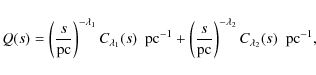
|
(52) |
where
We now keep the parameter given by Lépine & Bongiorno fixed so that our broken power-law model has only one free parameter: the wide binary density
![]() .
In Fig. 15 we show the best-fit model curves corresponding to
.
In Fig. 15 we show the best-fit model curves corresponding to
![]() pc-3.
The broken power-law model also gives a decent fit to the 2PCF inferred
from our total sample. (One should not be misled by large
discrepancy between the model and the CDD showing the cumulative difference between the 2PCF and the corresponding model curve.) With a goodness-of-fit of
pc-3.
The broken power-law model also gives a decent fit to the 2PCF inferred
from our total sample. (One should not be misled by large
discrepancy between the model and the CDD showing the cumulative difference between the 2PCF and the corresponding model curve.) With a goodness-of-fit of
![]() and a reduced chi-square of
and a reduced chi-square of
![]() ,
the broken power-law model provides a significantly worse bestfit to the data than our single power-law model.
Nevertheless, as the errors in the 2PCF are slightly underestimated, the model is not put into question until Q<0.001 (Press et al. 1992, their Sect. 15), and we conclude that the broken power-law distribution found by Lépine & Bongiorno (2007) can not be rejected with confidence either.
,
the broken power-law model provides a significantly worse bestfit to the data than our single power-law model.
Nevertheless, as the errors in the 2PCF are slightly underestimated, the model is not put into question until Q<0.001 (Press et al. 1992, their Sect. 15), and we conclude that the broken power-law distribution found by Lépine & Bongiorno (2007) can not be rejected with confidence either.
6.2 Internal (in)consistencies
Figure 10 shows that the best-fitting values for ![]() and
and
![]() are inconsistent, within the adopted random
errors, when the limiting magnitude is varied. Both parameters are
systematically shifted by roughly 20% when the limiting magnitude
is changed by 1 mag. Further inconsistencies were met when we
tried to differentiate our total sample with respect to colour
(not shown here). This very likely means that there are
unaccounted for systematic errors in the modelling, resting on oversimplified assumptions.
are inconsistent, within the adopted random
errors, when the limiting magnitude is varied. Both parameters are
systematically shifted by roughly 20% when the limiting magnitude
is changed by 1 mag. Further inconsistencies were met when we
tried to differentiate our total sample with respect to colour
(not shown here). This very likely means that there are
unaccounted for systematic errors in the modelling, resting on oversimplified assumptions.
A basic assumption on the properties of wide binaries was that both
components are drawn at random from the same stellar LF. There is,
however, some evidence that this is not quite correct: Gould et al. (1995) noticed
that ``binaries are bluer and more distant than one would expect if
they were formed of random combinations of field stars''. Also Lépine & Bongiorno (2007)
find ``that the luminosity function of the secondaries is significantly
different from that of the single stars field population, showing a
relative deficiency in low-luminosity (8<MV<14) objects''. Similarly, Sesar et al. (2008) report that blue stars (![]() mag, corresponding roughly to
mag, corresponding roughly to ![]() mag)
that are a member of a wide binary, have more blue companions than
expected from the LF. (For red stars, however, they find that the
components are drawn randomly from the LF.) Moreover, it has long
been known (e.g. Bahcall & Soneira 1980, their Fig. 2)
that stars of early spectral type have smaller scale heights than late
type stars; therefore, the assumption that the stellar density
distribution depends only on distance, and not on the luminosity of the
stars, might be an oversimplification as well.
mag)
that are a member of a wide binary, have more blue companions than
expected from the LF. (For red stars, however, they find that the
components are drawn randomly from the LF.) Moreover, it has long
been known (e.g. Bahcall & Soneira 1980, their Fig. 2)
that stars of early spectral type have smaller scale heights than late
type stars; therefore, the assumption that the stellar density
distribution depends only on distance, and not on the luminosity of the
stars, might be an oversimplification as well.
On the other hand, the internal inconsistency discussed is overemphasised in Fig. 10
because we only include the statistical errors stemming from the pair
counts when determining the MCCRs. If we also included the errors
in the Galactic structure parameters and those from the LF, the
MCCRs would be considerably larger, and the inconsistency evident from
Fig. 10 would not be as
severe as it seems. That a variation in the Galactic structure
parameter has a significant impact at least on
![]() ,
is apparent from Fig. 7. The systematic drift towards larger
,
is apparent from Fig. 7. The systematic drift towards larger ![]() and
and
![]() ,
when adopting a brighter upper apparent magnitude limit (cf. Fig. 10),
still points to some inconsistencies in our model.
We think, however, that these inconsistencies do not entirely undermine
our major results, although the quoted uncertainties might be
considerably larger.
,
when adopting a brighter upper apparent magnitude limit (cf. Fig. 10),
still points to some inconsistencies in our model.
We think, however, that these inconsistencies do not entirely undermine
our major results, although the quoted uncertainties might be
considerably larger.
7 Summary and conclusions
We have derived the angular 2PCF for nearly 670 000 SDSS stars brighter than r = 20.5 mag and redder than g-r =
0.5 mag in a region of approximately 670 square degrees
around the NGP. Various corrections had to be made for quasar
contamination, survey holes, and bright stars. There is an unambiguous
correlation signal on small scales up to 30
![]() .
We modelled this signal by a modified WW-technique, closely following a previous study of Garnavich (1991,1988)
that was based on a much smaller sample of stars. The modelling
involved a number of parametrised distribution functions: the spatial
density and LF of stars, as well as the separation distribution of
binaries. The Galactic model used is based on the recent study by Juric et al. (2008) and the stellar LF derived by Jahreiß & Wielen (1997).
For the wide binary semi-major axis distribution we assumed a single
powerlaw. Furthermore, essential assumptions are: (1) binary stars
follow the same density distribution as single stars; (2) both
components of a binary are randomly drawn from the single star
luminosiy function. These assumptions allowed a significant
simplification of the model. The Galactic structure parameters were
fixed (we explore three different sets), while the local wide
binary number density
.
We modelled this signal by a modified WW-technique, closely following a previous study of Garnavich (1991,1988)
that was based on a much smaller sample of stars. The modelling
involved a number of parametrised distribution functions: the spatial
density and LF of stars, as well as the separation distribution of
binaries. The Galactic model used is based on the recent study by Juric et al. (2008) and the stellar LF derived by Jahreiß & Wielen (1997).
For the wide binary semi-major axis distribution we assumed a single
powerlaw. Furthermore, essential assumptions are: (1) binary stars
follow the same density distribution as single stars; (2) both
components of a binary are randomly drawn from the single star
luminosiy function. These assumptions allowed a significant
simplification of the model. The Galactic structure parameters were
fixed (we explore three different sets), while the local wide
binary number density
![]() and the power-law index
and the power-law index ![]() of the semi-major axis distribution were left free; i.e., they have been determined by a least-squares fitting algorithm.
of the semi-major axis distribution were left free; i.e., they have been determined by a least-squares fitting algorithm.
The best fit to the observed angular 2PCF of the total sample was obtained with
![]() ,
which corresponds to the canonical Öpik law, and
,
which corresponds to the canonical Öpik law, and
![]() pc-3,
meaning an overall local wide binary fraction of about 10.0% in
the projected separation range of 0.001 pc (200 AU) to
1 pc (Galactic tidal limit). Previous studies (Sesar et al. 2008; Poveda & Allen 2004; Lépine & Bongiorno 2007) have also found the data to be consistent with Öpik's
law, but only to a maximal separation that is considerably smaller than
the Galactic tidal limit. Beyond that maximum separation, the
distribution continues with a steeper decline. We have shown that our
data are also consistent with the broken powerlaw found by Lépine & Bongiorno, although with a fit of lower quality (though involving only one free parameter, namely,
pc-3,
meaning an overall local wide binary fraction of about 10.0% in
the projected separation range of 0.001 pc (200 AU) to
1 pc (Galactic tidal limit). Previous studies (Sesar et al. 2008; Poveda & Allen 2004; Lépine & Bongiorno 2007) have also found the data to be consistent with Öpik's
law, but only to a maximal separation that is considerably smaller than
the Galactic tidal limit. Beyond that maximum separation, the
distribution continues with a steeper decline. We have shown that our
data are also consistent with the broken powerlaw found by Lépine & Bongiorno, although with a fit of lower quality (though involving only one free parameter, namely,
![]() ).
Given this ambiguity, we are not able to put any strong constraints on
the presence of a break in the wide binary separation distribution,
which is regarded as one of the most interesting aspects of wide
binaries. As to the wide binary fraction, we are in good accord
with Lépine & Bongiorno (2007), whereas an apparent discrepancy with Sesar et al. (2008) remains.
).
Given this ambiguity, we are not able to put any strong constraints on
the presence of a break in the wide binary separation distribution,
which is regarded as one of the most interesting aspects of wide
binaries. As to the wide binary fraction, we are in good accord
with Lépine & Bongiorno (2007), whereas an apparent discrepancy with Sesar et al. (2008) remains.
A differentiation of the sample with respect to limiting apparent magnitude turned up a systematic dependence of the binary parameters on the sample depth, which is most probably an artefact caused by oversimplified model assumptions. This conjecture is strengthened by the impossibility obtaining self-consistent results when differentiating with respect to colour. We conclude that one or more of the simplifying assumptions put into the model (e.g. that the luminosities of the binary components are independent of each other and draw randomly from the single-star LF or that binaries' density distribution follows exactly the single-star density distribution and that the density distribution is independent of the stars' luminosities) are not quite correct.
Differentiating the sample in terms of direction in the sky did yield some modest but non-significant variations. Only in one direction (subarea E) was an unexplained overdensity found.
While we have shown here that the stellar angular 2PCF, as a
complement to common proper motion studies, basically works and remains
a viable tool for the study of wide binaries, it has become clear
that this method is severely limited by the need for - even
more - complex modelling.
To relax those simple model assumptions would unduly complicate
the analysis much further and probably no longer yield unique
solutions. Any more efficient progress will indeed have to involve
distance information to discriminate against unwanted chance
projections. We plan to include distance information in our future
work. In spite of the limitations of the present, simple modelling
of the angular 2PCF, we think that the general result for the
total sample derived here, i.e.
![]() (Öpik law) and
(Öpik law) and
![]() among stars having a spectral type later than G5, to within an uncertainty of 10-20%, is a robust result.
among stars having a spectral type later than G5, to within an uncertainty of 10-20%, is a robust result.
Appendix A: Edge correction for holes
To quantify the edge effect from holes in our sample, we assume that
the holes are circular and flat (Euclidian) and that effects due to
intersecting holes are negligible. Let
![]() be the solid angle of the annulus of width
be the solid angle of the annulus of width ![]() around a hole of radius
around a hole of radius
![]()
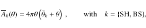
|
(A.1) |
where k stands for hole masks (survey holes: SH) or bright star masks (BS). Due to the holes in our sample we observe only a fraction
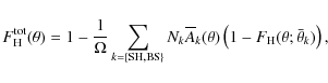
|
(A.2) |
where
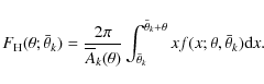
Here, f is the fraction of the area
|
(A.4) |
whereas
|
(A.5) |
where

|
(A.6) |
and
|
(A.7) |
Solving x=p+q for y using Maple gives
|
(A.8) |
where the integration in (A.3) was performed with Maple, too.
![\begin{figure}
\par\includegraphics[width=8.8cm,clip]{13109fA1.eps}
\end{figure}](/articles/aa/full_html/2010/01/aa13109-09/img249.png)
|
Figure A.1: Illustration of the
geometry used to correct for edge effects due to holes. The large
circle represents the bounding circle of a hole or a bright star mask.
A star lying close to the hole is indicated. The region within a
distance |
| Open with DEXTER | |
Appendix B: Galactic tidal limit
A crude estimate of the Galactic tidal limit ![]() ,
i.e. of the maximum semi-major axis
,
i.e. of the maximum semi-major axis ![]() of a binary star with total mass
of a binary star with total mass
![]() orbiting in the Galactic tidal field is provided by the Jacobi limit
orbiting in the Galactic tidal field is provided by the Jacobi limit ![]() (sometimes also referred to as zero-velocity surface or Roche sphere) (e.g. Binney & Tremaine 2008, Sect. 8.3)
(sometimes also referred to as zero-velocity surface or Roche sphere) (e.g. Binney & Tremaine 2008, Sect. 8.3)
|
(B.1) |
where
|
(B.2) |
where we have adopted the canonical value of the circular speed
For a rough estimate of this distance range, it is useful to define the effective depth of the sample as the most likely distance of an arbitrarly chosen star (Weinberg & Wasserman 1988).
In a magnitude-limited sample the total number of stars expected to be
observed in a (heliocentric) distance range between D and
![]() is
is
|
(B.3) |
where
where
|
(B.5) |
and
|
(B.6) |
In Table 2 we list the values of
| |
= | ||
| (B.7) |
Its values are typically somewhat above 8 kpc.
The last parameter we need to specify in order to estimate the Galactic tidal limit ![]() ,
is the total mass of the binary star
,
is the total mass of the binary star
![]() .
Given the magnitude limits of our sample we may write the average mass of a star in the sample as
.
Given the magnitude limits of our sample we may write the average mass of a star in the sample as
|
(B.8) |
where
Statistically, we expect the total mass of a binary star to be
![]() ,
and we finally estimate the Galactic tidal limit according to
,
and we finally estimate the Galactic tidal limit according to
| |
|
||
|
(B.9) |
The values of
We are grateful to P. M. Garnavich for providing us with his Ph.D. Thesis, which served as a starting point for our study. It is a pleasure to thank R. Buser, B. Krusche, T. Lisker, N. Sambhus, I. Sick, G. A. Tammann, C. von Arx, A. Willand, and T. Zingg for helpful comments and valuable discussions of the present work. We are much obliged to the referee for a prompt and insightful report. We are indebted to N. Peduzzi and the A&A language editor J. Adams for proofreading our manuscript. Funding for the SDSS and SDSS-II has been provided by the Alfred P. Sloan Foundation, the Participating Institutions, the National Science Foundation, the US Department of Energy, the National Aeronautics and Space Administration, the Japanese Monbukagakusho, the Max Planck Society, and the Higher Education Funding Council for England. The SDSS Web Site is http://www.sdss.org/. The SDSS is managed by the Astrophysical Research Consortium for the Participating Institutions. The Participating Institutions are the American Museum of Natural History, Astrophysical Institute Potsdam, University of Basel, University of Cambridge, Case Western Reserve University, University of Chicago, Drexel University, Fermilab, the Institute for Advanced Study, the Japan Participation Group, Johns Hopkins University, the Joint Institute for Nuclear Astrophysics, the Kavli Institute for Particle Astrophysics and Cosmology, the Korean Scientist Group, the Chinese Academy of Sciences (LAMOST), Los Alamos National Laboratory, the Max-Planck-Institute for Astronomy (MPIA), the Max-Planck-Institute for Astrophysics (MPA), New Mexico State University, Ohio State University, University of Pittsburgh, University of Portsmouth, Princeton University, the United States Naval Observatory, and the University of Washington. This work was supported by the Swiss National Science Foundation.
References
- Abt, H. A. 1983, ARA&A, 21, 343 [Google Scholar]
- Adelman-McCarthy, J. K., Agüeros, M. A., Allam, S. S., et al. 2007, ApJS, 172, 634 [NASA ADS] [CrossRef] [Google Scholar]
- Adelman-McCarthy, J. K., Agüeros, M. A., Allam, S. S., et al. 2008, ApJS, 175, 297 [NASA ADS] [CrossRef] [Google Scholar]
- Allen, C., Poveda, A., & Hernández-Alcántara, A. 2007, in IAU Symp. 240, ed. W. I. Hartkopf, E. F. Guinan, & P. Harmanec, 405 [Google Scholar]
- Bahcall, J. N., & Soneira, R. M. 1980, ApJS, 44, 73 [NASA ADS] [CrossRef] [Google Scholar]
- Bahcall, J. N., & Soneira, R. M. 1981, ApJ, 246, 122 [NASA ADS] [CrossRef] [Google Scholar]
- Bahcall, J. N., Hut, P., & Tremaine, S. 1985a, ApJ, 290, 15 [NASA ADS] [CrossRef] [Google Scholar]
- Bahcall, J. N., Ratnatunga, K. U., Buser, R., Fenkart, R. P., & Spaenhauer, A. 1985b, ApJ, 299, 616 [NASA ADS] [CrossRef] [Google Scholar]
- Bernstein, G. M. 1994, ApJ, 424, 569 [NASA ADS] [CrossRef] [Google Scholar]
- Bilir, S., Karaali, S., & Tunçel, S. 2005, Astron. Nachr., 326, 321 [NASA ADS] [CrossRef] [Google Scholar]
- Binney, J., & Tremaine, S. 2008, Galactic Dynamics: Second Edition, ed. J. Binney, & S. Tremaine (Princeton University Press) [Google Scholar]
- Chanamé, J. 2007, in IAU Symp. 240, ed. W. I. Hartkopf, E. F. Guinan, & P. Harmanec, 316 [Google Scholar]
- Chanamé, J., & Gould, A. 2004, ApJ, 601, 289 [NASA ADS] [CrossRef] [Google Scholar]
- Chen, B., Stoughton, C., Smith, J. A., et al. 2001, ApJ, 553, 184 [NASA ADS] [CrossRef] [Google Scholar]
- Close, L. M., Richer, H. B., & Crabtree, D. R. 1990, AJ, 100, 1968 [NASA ADS] [CrossRef] [Google Scholar]
- Doinidis, S. P., & Beers, T. C. 1989, ApJ, 340, L57 [NASA ADS] [CrossRef] [Google Scholar]
- Finlator, K., Ivezic, Z., Fan, X., et al. 2000, AJ, 120, 2615 [NASA ADS] [CrossRef] [Google Scholar]
- Garnavich, P. M. 1988, ApJ, 335, L47 [NASA ADS] [CrossRef] [Google Scholar]
- Garnavich, P. M. 1991, Ph.D. Thesis, AA, Washington Univ., Saint Louis, MO. [Google Scholar]
- Gomez, M., & Lada, C. J. 1998, AJ, 115, 1524 [NASA ADS] [CrossRef] [Google Scholar]
- Goodwin, S. P., Kroupa, P., Goodman, A., & Burkert, A. 2007, in Protostars and Planets V, ed. B. Reipurth, D. Jewitt, & K. Keil, 133 [Google Scholar]
- Gould, A., Bahcall, J. N., Maoz, D., & Yanny, B. 1995, ApJ, 441, 200 [NASA ADS] [CrossRef] [Google Scholar]
- Gunn, J. E., Carr, M., Rockosi, C., et al. 1998, AJ, 116, 3040 [NASA ADS] [CrossRef] [Google Scholar]
- Hamilton, A. J. S. 1993, ApJ, 417, 19 [NASA ADS] [CrossRef] [Google Scholar]
- Harris, H. C., Munn, J. A., Kilic, M., et al. 2006, AJ, 131, 571 [NASA ADS] [CrossRef] [Google Scholar]
- Hernandez, X., & Lee, W. H. 2008, MNRAS, 387, 1727 [NASA ADS] [CrossRef] [Google Scholar]
- Jahreiß, H., & Wielen, R. 1997, in Hipparcos - Venice '97, ESA SP-402, 675 [Google Scholar]
- Juric, M., Ivezic, Z., Brooks, A., et al. 2008, ApJ, 673, 864 [NASA ADS] [CrossRef] [MathSciNet] [Google Scholar]
- Karttunen, H., Kröger, P., Oja, H., Poutanen, M., & Donner, K. J. 1996, Fundamental Astronomy, ed. H. Karttunen, P. Kröger, H. Oja, M. Poutanen, & K. J. Donner [Google Scholar]
- Kobulnicky, H. A., & Fryer, C. L. 2007, ApJ, 670, 747 [NASA ADS] [CrossRef] [Google Scholar]
- Kroupa, P., Tout, C. A., & Gilmore, G. 1993, MNRAS, 262, 545 [NASA ADS] [CrossRef] [Google Scholar]
- Laird, J. B., Carney, B. W., & Latham, D. W. 1988, AJ, 95, 1843 [NASA ADS] [CrossRef] [Google Scholar]
- Larson, R. B. 2001, in The Formation of Binary Stars, ed. H. Zinnecker, & R. Mathieu, IAU Symp., 200, 93 [Google Scholar]
- Latham, D. W., Schechter, P., Tonry, J., Bahcall, J. N., & Soneira, R. M. 1984, ApJ, 281, L41 [NASA ADS] [CrossRef] [Google Scholar]
- Latham, D. W., Stefanik, R. P., Torres, G., et al. 2002, AJ, 124, 1144 [NASA ADS] [CrossRef] [Google Scholar]
- Lépine, S., & Bongiorno, B. 2007, AJ, 133, 889 [NASA ADS] [CrossRef] [Google Scholar]
- López-Corredoira, M., Garzón, F., Hammersley, P. L., & Mahoney, T. J. 1998, MNRAS, 301, 289 [NASA ADS] [CrossRef] [Google Scholar]
- Lourakis, M. 2004, levmar: Levenberg-Marquardt nonlinear least squares algorithms in C/C++, http://www.ics.forth.gr/ lourakis/levmar/ [Google Scholar]
- Lupton, R., Gunn, J. E., Ivezic, Z., Knapp, G. R., & Kent, S. 2001, in Astronomical Data Analysis Software and Systems X, ed. F. R. Harnden, Jr., F. A. Primini, & H. E. Payne, ASP Conf. Ser., 238, 269 [Google Scholar]
- Milgrom, M., & Bekenstein, J. 1987, in Dark matter in the universe, ed. J. Kormendy, & G. R. Knapp, IAU Symp., 117, 319 [Google Scholar]
- Öpik, E. 1924, Publications of the Tartu Astrofizica Observatory, 25, 1 [Google Scholar]
- Parker, R. J., Goodwin, S. P., Kroupa, P., & Kouwenhoven, M. B. N. 2009, MNRAS, 873 [Google Scholar]
- Peebles, P. J. E. 1980, The large-scale structure of the universe, Research supported by the National Science Foundation (Princeton, N.J.: Princeton University Press), 435 [Google Scholar]
- Poveda, A., & Allen, C. 2004, in Rev. Mex. Astron. Astrofis. Conf. Ser. 21, ed. C. Allen, & C. Scarfe, 49 [Google Scholar]
- Poveda, A., Allen, C., & Hernández-Alcántara, A. 2007, in IAU Symp. 240, ed. W. I. Hartkopf, E. F. Guinan, & P. Harmanec, 417 [Google Scholar]
- Poveda, A., Herrera, M. A., Allen, C., Cordero, G., & Lavalley, C. 1994, Rev. Mex. Astron. Astrofis., 28, 43 [NASA ADS] [Google Scholar]
- Press, W. H., Teukolsky, S. A., Vetterling, W. T., & Flannery, B. P. 1992, Numerical recipes in C. The art of scientific computing (Cambridge: University Press), 2nd edn. [Google Scholar]
- Quinn, D. P., Wilkinson, M. I., Irwin, M. J., et al. 2009, MNRAS, 396, L11 [NASA ADS] [CrossRef] [Google Scholar]
- Reid, I. N., & Gizis, J. E. 1997, AJ, 113, 2246 [NASA ADS] [CrossRef] [Google Scholar]
- Retterer, J. M., & King, I. R. 1982, ApJ, 254, 214 [NASA ADS] [CrossRef] [Google Scholar]
- Saarinen, S., & Gilmore, G. 1989, MNRAS, 237, 311 [NASA ADS] [CrossRef] [Google Scholar]
- Schlegel, D. J., Finkbeiner, D. P., & Davis, M. 1998, ApJ, 500, 525 [NASA ADS] [CrossRef] [Google Scholar]
- Scranton, R., Johnston, D., Dodelson, S., et al. 2002, ApJ, 579, 48 [NASA ADS] [CrossRef] [Google Scholar]
- Sesar, B., Ivezic, Z., & Juric, M. 2008, ApJ, 689, 1244 [NASA ADS] [CrossRef] [Google Scholar]
- Valtonen, M. 1997, Celest. Mech. Dyn. Astron., 68, 27 [NASA ADS] [CrossRef] [Google Scholar]
- Wasserman, I. & Weinberg, M. D. 1987, ApJ, 312, 390 (WW87) [NASA ADS] [CrossRef] [Google Scholar]
- Wasserman, I., & Weinberg, M. D. 1991, ApJ, 382, 149 [NASA ADS] [CrossRef] [Google Scholar]
- Weinberg, M. D. 1988, Ap&SS, 142, 277 [Google Scholar]
- Weinberg, M. D. 1990, in Baryonic Dark Matter, NATO ASIC Proc., 305, 117 [Google Scholar]
- Weinberg, M. D., & Wasserman, I. 1988, ApJ, 329, 253 [NASA ADS] [CrossRef] [Google Scholar]
- Weinberg, M. D., Shapiro, S. L., & Wasserman, I. 1987, ApJ, 312, 367 [NASA ADS] [CrossRef] [Google Scholar]
- Yoo, J., Chanamé, J., & Gould, A. 2004, ApJ, 601, 311 [NASA ADS] [CrossRef] [Google Scholar]
- York, D. G., Adelman, J., Anderson, Jr., J. E., et al. 2000, AJ, 120, 1579 [Google Scholar]
Footnotes
- ...
primary
![[*]](/icons/foot_motif.png)
- Due to overlaps in the imaging, many objects are observed more than once. The best of those observations is called the primary object, all the others are called secondary objects.
- ... view
- See cas.sdss.org/dr6/en/help/browser/browser.asp
- ... PSF magnitude
- See sdss.org/dr6/algorithms/photometry.html#mag_psf
- ... recommendations
- See sdss.org/dr6/products/catalogs/flags.html
- ... photometry
- See cas.sdss.org/dr6/en/help/docs/realquery.asp#flags
- ...)
- See also astro.princeton.edu/PBOOK/camera/camera.htm
- ...)
- See also sdss.org/dr6/products/general/stargalsep.html
- ...)
- See also sdss.org/dr6/
- ...(Adelman-McCarthy
et al.
2008)
- See also http://www.sdss.org/dr6/ and the DR5 paper (Adelman-McCarthy et al. 2007).
- ... table
- See cas.sdss.org/dr6/en/help/docs/algorithm.asp?key=qsocat
- ... masked
- See sdss.org/dr6/algorithms/masks.html
- ... neighbourhood
- We use the term ``solar neighbourhood'' for local quantities.
- ...(Lourakis 2004)
- We use levmar-2.2.
- ... unrealistic
- ``Physically, one doesn't expect to see a sharp cutoff.'' (Weinberg 1990).
All Tables
Table 1: Galactic structure parameters.
Table 2: Parameters of the final sample and of the subsamples.
Table 3: Best-fit values: total sample.
Table 4: Best-fit values: r<20.0 mag and r<19.5 mag.
Table 5: Best-fit values: left and right.
Table 6: Best-fit values: A to H.
Table 7: Best-fit values: excluding subsample E.
All Figures
|
|
Figure 1: Distribution of stars (grey points filling the background) in our total sample. Black asterisks show the positions of bright star masks, white circles those of hole masks. The size of the symbols are not to scale. |
| Open with DEXTER | |
| In the text | |
|
|
Figure 2: Colour-colour diagram of all point-like objects within our coordinate's and apparent magnitude's limits (grey points). Black points are SDSS quasar candidates. The vertical dashed line indicates the cut at g-r=0.5 mag (see text). Approximate spectral classes are indicated. |
| Open with DEXTER | |
| In the text | |
|
|
Figure 3: 2PCF as inferred from a random sample (solid circles, left ordinate) and the corresponding CDD (open circles, right ordinate). Poisson errors are indicated as vertical lines. |
| Open with DEXTER | |
| In the text | |
|
|
Figure 4: Effective volumes calculated using the parameters that correspond to our final sample (Table 2) for the three Galactic structure parameter sets as discussed in Sect. 4.2. Long dashed line: set 1; solid line: set 2; short dashed line: set 3. |
| Open with DEXTER | |
| In the text | |
|
|
Figure 5: 2PCF as inferred from the total sample (solid circles, left ordinate) and the corresponding CDD (open circles, right ordinate). Poisson errors are indicated as vertical lines. Model curves for the three Galactic structure parameter sets are plotted, too, but as the differences between them are marginal they lie one upon the other, giving a single solid line. |
| Open with DEXTER | |
| In the text | |
|
|
Figure 6:
Distribution of the best-fit values for the total sample using the
structure parameter set 2 obtained by the Monte Carlo
procedure described in the text. The solid contours (MCCRs) are lines
of constant |
| Open with DEXTER | |
| In the text | |
|
|
Figure 7:
MCCRs for the three Galactic structure parameter sets corresponding to
the total sample. Long dashed line: set 1; solid line: set 2;
short dashed line: set 3. The crosses indicate the best-fit values
inferred from the true observed number of pairs,
|
| Open with DEXTER | |
| In the text | |
|
|
Figure 8: Distribution of wide binaries as a function of projected separation s that is expected to be observed in the total sample, given the model assumptions and the selection criteria we have adopted (see text). |
| Open with DEXTER | |
| In the text | |
|
|
Figure 9:
2PCF and CDD for the r<20.0 mag and r<19.5 mag
subsamples together with the corresponding model curves. Up-pointing
triangles (long-dashed lines) are for the r<20.0 mag subsample, whereas down-pointing triangles (short-dashed lines) are for the r<19.5 mag subsample. The symbols were shifted apart by
|
| Open with DEXTER | |
| In the text | |
|
|
Figure 10: MCCRs for the r<20.0 mag (long dashed contours) and r<19.5 mag (short-dashed contours) subsamples. For comparison, the MCCR for our final sample is also shown (solid-contours). The crosses have the same meaning as in Fig. 7. |
| Open with DEXTER | |
| In the text | |
|
|
Figure 11: 2PCF and CDD for the
left and the right subsamples, together with the corresponding model
curves. Left-pointing triangles (long-dashed lines) are for the left
subsample, whereas right-pointing triangles (short-dashed lines) are
for the right subsample. The symbols were shifted apart by
|
| Open with DEXTER | |
| In the text | |
|
|
Figure 12: MCCRs for the left (long-dashed contours) and right (short-dashed contours) subsamples. For comparison, also the MCCR for our final sample is shown (solid contours). The crosses have the same meaning as in Fig. 7. |
| Open with DEXTER | |
| In the text | |
|
|
Figure 13: 2PCF (solid circles) and CDD (open circles) for the subsamples A to H, together with the corresponding model curves. The subfigures are arranged as the corresponding subareas would be seen on the sky. |
| Open with DEXTER | |
| In the text | |
|
|
Figure 14: 95.4% MCCRs for the subsamples A to H. The crosses have the same meaning as in Fig. 7. |
| Open with DEXTER | |
| In the text | |
|
|
Figure 15: 2PCF and CDD as inferred from our total sample as in Fig. 5. The model curve is for the broken power-law model from Lépine & Bongiorno (2007) (see text). |
| Open with DEXTER | |
| In the text | |
|
|
Figure A.1: Illustration of the
geometry used to correct for edge effects due to holes. The large
circle represents the bounding circle of a hole or a bright star mask.
A star lying close to the hole is indicated. The region within a
distance |
| Open with DEXTER | |
| In the text | |
Copyright ESO 2010
Current usage metrics show cumulative count of Article Views (full-text article views including HTML views, PDF and ePub downloads, according to the available data) and Abstracts Views on Vision4Press platform.
Data correspond to usage on the plateform after 2015. The current usage metrics is available 48-96 hours after online publication and is updated daily on week days.
Initial download of the metrics may take a while.