| Issue |
A&A
Volume 509, January 2010
|
|
|---|---|---|
| Article Number | A32 | |
| Number of page(s) | 11 | |
| Section | Stellar structure and evolution | |
| DOI | https://doi.org/10.1051/0004-6361/200913103 | |
| Published online | 14 January 2010 | |
Exploring the P vs. P
vs. P relation with flux transport dynamo models of solar-like stars
L. Jouve1,2 - B. P. Brown3 - A. S. Brun1,3
1 - Laboratoire AIM, CEA/DSM-CNRS-Université Paris Diderot,
IRFU/SAp, 91191 Gif-sur-Yvette, France
2 -
D.A.M.T.P., Centre for Mathematical Sciences, University of Cambridge, Cambridge CB03 0WA, UK
3 -
JILA and Department of Astrophysical and Planetary Sciences, University of Colorado, Boulder, CO 80309-0440, USA
Received 11 August 2009 / Accepted 5 November 2009
Abstract
Aims. Understand stellar magnetism and test the validity of
the Babcock-Leighton flux transport mean field dynamo models with
stellar activity observations
Methods. 2-D mean field dynamo models at various rotation rates
are computed with the STELEM code to study the sensitivity of the
activity cycle period and butterfly diagram to parameter changes and
are compared to observational data. The novelty is that these 2-D mean
field dynamo models incorporate scaling laws deduced from 3-D
hydrodynamical simulations for the influence of rotation rate on the
amplitude and profile of the meridional circulation. These models make
also use of observational scaling laws for the variation of
differential rotation with rotation rate.
Results. We find that Babcock-Leighton flux transport dynamo
models are able to reproduce the change in topology of the magnetic
field (i.e. toward being more toroidal with increasing rotation rate)
but seem to have difficulty reproducing the cycle period vs activity
period correlation observed in solar-like stars if a monolithic single
cell meridional flow is assumed. It may however be possible to recover
the
![]() vs.
vs.
![]() relation with more complex meridional flows, if the profile changes in a particular assumed manner with rotation rate.
relation with more complex meridional flows, if the profile changes in a particular assumed manner with rotation rate.
Conclusions. The Babcock-Leighton flux transport dynamo model based on single cell meridional circulation does not reproduce the
![]() vs.
vs.
![]() relation unless the amplitude of the meridional circulation is assumed
to increase with rotation rate which seems to be in contradiction with
recent results obtained with 3-D global simulations.
relation unless the amplitude of the meridional circulation is assumed
to increase with rotation rate which seems to be in contradiction with
recent results obtained with 3-D global simulations.
Key words: magnetohydrodynamics - stars: activity - stars: magnetic fields - Sun: activity - methods: numerical
1 Introduction
The Sun is a magnetic star that possesses a well defined cyclic activity period of 22 years. It is believed that the origin of this magnetism and regular activity is linked to a global scale dynamo operating in and at the base of the solar convection zone (Parker 1993). In order to model and understand this global scale dynamo, a useful approach has been to make use of the mean field dynamo theory (Moffatt 1978; Krause & Raedler 1980). This method has the advantage that it only deals with the large scale magnetic field, assuming some parameterization of the underlying small scale turbulence and magnetism. Computing those physical processes self-consistently would otherwise require costly full 3-D magnetohydrodynamical (MHD) simulations (Cattaneo 1999; Brun et al. 2004). Among the various mean field dynamo models, the Babcock-Leighton flux transport dynamo models have recently been the favored ones and have demonstrated some success at reproducing solar observations assuming either an advection or a diffusion dominated regime for the transport of field from the surface down to the tachocline (Dikpati & Charbonneau 1999; Nandy & Choudhuri 2002; Dikpati et al. 2004; Chatterjee et al. 2004; Charbonneau 2005; Bonanno et al. 2005; Jouve & Brun 2007a; Yeates et al. 2008).It is legitimate to ask if such models can be applied to other stars and lead to the same agreement with the observations of for instance solar type stars that may possess different rotation rates and activity levels.
1.1 Observational constraints
Observations of the magnetism of ``solar type'' stars, i.e. stars possessing a deep convective envelope and a radiative interior (late F, G, K and early M spectral type) are becoming more and more available (Giampapa 2004) and may provide additional constraints on our understanding of global scale stellar dynamos. One difficulty of such observational programs is that they require long term observations since stellar cycle periods are likely to be commensurate to the solar 11-yr sunspots cycle period (or 22-yr for a full cycle including two polarity reversals of the global poloidal field). Thanks to the data collected at Mount Wilson Observatory since the late 60's, such data is available (Wilson 1978; Baliunas et al. 1995). Among the sample of 111 stars (including the Sun as a star) originally observed between the F2 to M2 spectral type, it is found that about 50% of the stars possess a cyclic activity, with cycle (starspot) periods varying roughly between 5 to 25 yrs, i.e. between half to twice the sunspot cycle period. They further indicate that among the inactive stars of the sample some are likely to be in a quiet phase (as was the Sun during the Maunder minimum). Overall activity cycles seems to be more frequent for less massive stars K than for F stars. More recent observational programs have been pursued that now even provide information on the field topology as a function of the rotation rate, such as the one using the Espadons and Narval instruments and the Zeeman Doppler Imaging technique (Donati et al. 2006). Applying this observational technique over a sample of four solar analogues with rotation rate varying from one to three times solar, Petit et al. (2008) have shown that the field amplitude increases as a function of the star's rotation rate and, more importantly, becomes more and more dominated by its toroidal component (modulo possible bias in the observational technique used). If such a trend is confirmed, i.e. that the field topology is becoming more toroidal with increasing rotation rate, it is a very important and instructive result and puts strong constraints on the dynamo models.
The systematic analysis of stellar magnetism data revealed that for solar type stars there is a good correlation
between the cycle and rotation periods of the stars and that correlation is even stronger
when using the Rossby number (
![]() )
that takes into account the convection turnover time
)
that takes into account the convection turnover time ![]() at the base
of the stellar convective envelope (Noyes et al. 1984; Soon et al. 1993; Hempelmann et al. 1995; Baliunas et al. 1996).
As the star rotates faster, its cycle period is found to be shorter. Typically Noyes et al. (1984) found that
at the base
of the stellar convective envelope (Noyes et al. 1984; Soon et al. 1993; Hempelmann et al. 1995; Baliunas et al. 1996).
As the star rotates faster, its cycle period is found to be shorter. Typically Noyes et al. (1984) found that
![]() ,
with
,
with
![]() .
Based on an extended stellar sample Saar & Brandenburg (1999) and Saar (2002) have argued that there is actually two branches when plotting the cycle period vs. the rotation
period of the stars. They make the distinction between the primary (starspot) cycle and Gleissberg or grand minima
type modulation of the stellar activity. For the active branch they found an exponent
.
Based on an extended stellar sample Saar & Brandenburg (1999) and Saar (2002) have argued that there is actually two branches when plotting the cycle period vs. the rotation
period of the stars. They make the distinction between the primary (starspot) cycle and Gleissberg or grand minima
type modulation of the stellar activity. For the active branch they found an exponent
![]() and for the inactive stars
and for the inactive stars
![]() (Charbonneau & Saar 2001).
It is also found that this correlation breaks
at high rotation rate with the possible appearance of a super active
branch. Further at very high rotation rate saturation of the X-ray
luminosity seems to limit the validity of the scaling found at more
moderate rotation rates (Pizzolato et al. 2003). For G type stars
this saturation is found for rotation rate above 35 km s-1, for K type stars at about 10 km s-1 and for M dwarfs around
3-4 km s-1 (Browning 2008; Reiners et al. 2009). How stellar magnetic flux scales with rotation rate is thus also important
to understand since it is telling us how the magnetic field generated by dynamo action inside the stars emerges and imprints
the stellar surface (Rempel 2008) and if it actually saturates.
(Charbonneau & Saar 2001).
It is also found that this correlation breaks
at high rotation rate with the possible appearance of a super active
branch. Further at very high rotation rate saturation of the X-ray
luminosity seems to limit the validity of the scaling found at more
moderate rotation rates (Pizzolato et al. 2003). For G type stars
this saturation is found for rotation rate above 35 km s-1, for K type stars at about 10 km s-1 and for M dwarfs around
3-4 km s-1 (Browning 2008; Reiners et al. 2009). How stellar magnetic flux scales with rotation rate is thus also important
to understand since it is telling us how the magnetic field generated by dynamo action inside the stars emerges and imprints
the stellar surface (Rempel 2008) and if it actually saturates.
1.2 Possible theoretical interpretation
Theoretical considerations to interpret stellar magnetism based on classical mean field ![]() -
-![]() dynamo models (Durney & Latour 1976; Knobloch et al. 1981; Baliunas et al. 1996)
naturally find correlation between rotation rate and stellar activity.
In particular it is found that both magnetic field generation and the
dynamo number D
(i.e. a Reynolds number characterizing the mean field
dynamo models (Durney & Latour 1976; Knobloch et al. 1981; Baliunas et al. 1996)
naturally find correlation between rotation rate and stellar activity.
In particular it is found that both magnetic field generation and the
dynamo number D
(i.e. a Reynolds number characterizing the mean field ![]() and
and ![]() dynamo
effects used in the models) vary with the rotation period of the star.
This is due to the fact that in these models both effects are sensitive
to
the rotation rate of the star. The
dynamo
effects used in the models) vary with the rotation period of the star.
This is due to the fact that in these models both effects are sensitive
to
the rotation rate of the star. The ![]() -effect is a direct measure of the differential rotation
-effect is a direct measure of the differential rotation
![]() established
in the star. It is well known both theoretically and observationally
that the differential rotation in the convective envelope of
solar-type stars is directly connected to the star's rotation rate
established
in the star. It is well known both theoretically and observationally
that the differential rotation in the convective envelope of
solar-type stars is directly connected to the star's rotation rate ![]() (Donahue et al. 1996; Barnes et al. 2005; Ballot et al. 2007;
Brown et al. 2008; Küker & Rüdiger 2008). However, the exact scaling
(Donahue et al. 1996; Barnes et al. 2005; Ballot et al. 2007;
Brown et al. 2008; Küker & Rüdiger 2008). However, the exact scaling ![]() (i.e.
(i.e.
![]() )
is still a matter of debate among the observers and theoreticians,
being sensitive to the observational techniques used and to the
modelling approach.
)
is still a matter of debate among the observers and theoreticians,
being sensitive to the observational techniques used and to the
modelling approach.
The ![]() -effect
used in mean field theory is related to helical turbulence and
represents a measure or parameterization of the mean electromotive
force (emf) (Moffatt 1978; Pouquet et al. 1976). It is thus also linked to the
rotation rate of the star and the amount of kinetic helicity present in its convective envelope.
However in Babcock-Leighton flux transport dynamo models the standard
-effect
used in mean field theory is related to helical turbulence and
represents a measure or parameterization of the mean electromotive
force (emf) (Moffatt 1978; Pouquet et al. 1976). It is thus also linked to the
rotation rate of the star and the amount of kinetic helicity present in its convective envelope.
However in Babcock-Leighton flux transport dynamo models the standard ![]() -effect is replaced by a surface term linked to the
tilt of the active regions with respect to the east-west direction (i.e. Joy's law, Kosovichev & Stenflo 2008). This tilt is thought
to be due to the action of the Coriolis force during the rise of the toroidal structures that emerge as active regions
(D'Silva & Choudhuri 1993). Recent 3-D simulations in spherical shells (Fan 2008; Jouve & Brun 2007b, 2009)
seem to indicate
that this is not the only effect responsible for the observed tilt and
that the twist and arching of the toroidal structures as well as the
continuous action of the surface convection during the emergence have
some influence on the resulting tilt. Thus the
dependence with rotation rate of the Babcock-Leighton surface source
term used in this class of mean field dynamo models is not
straightforward
to assess and needs to be studied in detail.
-effect is replaced by a surface term linked to the
tilt of the active regions with respect to the east-west direction (i.e. Joy's law, Kosovichev & Stenflo 2008). This tilt is thought
to be due to the action of the Coriolis force during the rise of the toroidal structures that emerge as active regions
(D'Silva & Choudhuri 1993). Recent 3-D simulations in spherical shells (Fan 2008; Jouve & Brun 2007b, 2009)
seem to indicate
that this is not the only effect responsible for the observed tilt and
that the twist and arching of the toroidal structures as well as the
continuous action of the surface convection during the emergence have
some influence on the resulting tilt. Thus the
dependence with rotation rate of the Babcock-Leighton surface source
term used in this class of mean field dynamo models is not
straightforward
to assess and needs to be studied in detail.
Another important ingredient in flux transport models is the large
scale meridional circulation (MC) used to connect the surface source
term generating
the poloidal field to the region of strong shear at the base of the
convection zone (i.e. the tachocline) where it will be subsequently
sheared
by the ![]() -effect in order to close the global dynamo loop (i.e.
-effect in order to close the global dynamo loop (i.e.
![]() ).
The meridional flow (or ``conveyor belt'') thus plays an important role
in setting the cycle period of the global dynamo in this class of flux
transport model. As a direct consequence it is natural to ask how the
meridional circulation amplitude and profile change with
the rotation rate and how these may influence the magnetic cycle
period.
).
The meridional flow (or ``conveyor belt'') thus plays an important role
in setting the cycle period of the global dynamo in this class of flux
transport model. As a direct consequence it is natural to ask how the
meridional circulation amplitude and profile change with
the rotation rate and how these may influence the magnetic cycle
period.
Early work by Dikpati et al. (2001)
have assumed that the amplitude of the meridional flow is proportional
to the rotation rate of the star. With such scaling they seem to be
able to reproduce some of the
rotation vs cycle period correlation observed in solar type stars.
Charbonneau & Saar (2001)
have also studied the sensitivity of various
mean field dynamo models in reproducing stellar activity observations
assuming for the Babcock-Leighton type that the meridional flow
amplitude increases either as ![]() or
as
or
as
![]() .
Similarly Nandy (2004) and Nandy & Martens (2007)
have explored the solar-stellar connection with B-L mean field dynamo
models and have
reached the same conclusion: only a positive scaling of the amplitude
of meridional flows with the rotation rate can reconcile the models
with observations of magnetism of solar-like stars.
However recent theoretical work by Ballot et al. (2007) and
Brown et al. (2008) indicate that this is unlikely to be the right scaling. Instead 3-D simulations reveal that the amplitude of the meridional
flow weakens as the rotation rate is increased.
.
Similarly Nandy (2004) and Nandy & Martens (2007)
have explored the solar-stellar connection with B-L mean field dynamo
models and have
reached the same conclusion: only a positive scaling of the amplitude
of meridional flows with the rotation rate can reconcile the models
with observations of magnetism of solar-like stars.
However recent theoretical work by Ballot et al. (2007) and
Brown et al. (2008) indicate that this is unlikely to be the right scaling. Instead 3-D simulations reveal that the amplitude of the meridional
flow weakens as the rotation rate is increased.
In this paper we wish to revisit the solar-stellar connection in the light of the latest theoretical and observational work done in the community. We have thus designed a series of Babcock-Leighton models with the STELEM code (Emonet & Charbonneau 1998, private communication; Jouve & Brun 2007a) that incorporate recent 3-D MHD results. By doing so we will study how these mean field models, quite successful at modelling the solar cycle, perform to explain the observed magnetic activity, cycle and field topology of solar type stars at various rotation rates. In Sect. 2 we discuss the 2-D mean field models used in this study and the way we incorporate 3-D results obtained with the ASH code (Clune et al. 1999; Brun et al. 2004). In Sect. 3 we present our series of stellar mean field dynamo models, while in Sect. 4 we vary the input parameters to evaluate the robustness of our results. In Sect. 5 we discuss and put in perspective our results.
2 The models and method
2.1 The model equation
To model the solar global dynamo operating in solar like stars, we use the hydromagnetic induction equation, governing the evolution of the magnetic field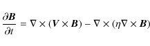
|
(1) |
where
As we are working in the framework of mean-field theory, we express both magnetic and velocity fields as a sum
of large-scale (that will correspond to mean field) and small-scale (associated with fluid turbulence) contributions.
Averaging over some suitably chosen intermediate scale makes it possible to write two distinct induction equations for
the mean and the fluctuating parts of the magnetic field. The mean-field equation reads:
| |
= | ||
| (2) |
where
Working in spherical coordinates and under the assumption of axisymmetry, we write the total mean magnetic field B
and velocity field V as (for the sake of simplicity we omit
![]() in the rest of the paper):
in the rest of the paper):
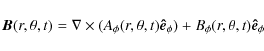
|
(3) |
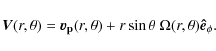
|
(4) |
Note that our velocity field is time-independent since we will not assume any fluctuations in time of the differential rotation
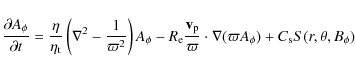
where
Equations (5) and (6)
are solved with the STELEM code (Emonet & Charbonneau 1998, private
communication) in an annular meridional plane with the colatitude ![]()
![]() and the
radius (in dimensionless units)
and the
radius (in dimensionless units)
![]() i.e. from slightly below the tachocline (r=0.7)
up to the solar surface.
The STELEM code has been thoroughly tested and validated thanks to an
international mean field dynamo benchmark involving 8 different
codes (Jouve et al. 2008).
At
i.e. from slightly below the tachocline (r=0.7)
up to the solar surface.
The STELEM code has been thoroughly tested and validated thanks to an
international mean field dynamo benchmark involving 8 different
codes (Jouve et al. 2008).
At ![]() and
and
![]() boundaries, both
boundaries, both ![]() and
and ![]() are set to 0. Both
are set to 0. Both ![]() and
and ![]() are set
to 0 at r=0.6. At the upper boundary, we smoothly match our solution to an external potential field, i.e. we have vacuum
for
are set
to 0 at r=0.6. At the upper boundary, we smoothly match our solution to an external potential field, i.e. we have vacuum
for ![]() .
As initial conditions we are setting a confined dipolar field configuration, i.e. the poloidal field is set to
.
As initial conditions we are setting a confined dipolar field configuration, i.e. the poloidal field is set to
![]() in
the convective zone and to 0 below the tachocline whereas the toroidal field is set to 0 everywhere.
in
the convective zone and to 0 below the tachocline whereas the toroidal field is set to 0 everywhere.
2.2 The physical ingredients
The rotation profile used in the series of models discussed in this
work captures some realistic aspects of the Sun's angular velocity,
deduced from helioseismic inversions (Thompson et al. 2003). We are thus
assuming a solid rotation below 0.66 and a differential rotation above the interface (cf. top panel of Fig. 1).
| |
= | ![$\displaystyle \Omega_{\rm c}+\frac{1}{2}\left[1+{\rm erf}(2\frac{r-r_{\rm c}}{d_{1}})\right]$](/articles/aa/full_html/2010/01/aa13103-09/img70.png)
|
|
| (7) |
with
![\begin{figure}
\par\includegraphics[width=7cm,clip]{13103f1a.ps}\par\vspace*{2mm}
\hspace*{2mm}\includegraphics[width=6.3cm,clip]{13103f1b.ps}
\end{figure}](/articles/aa/full_html/2010/01/aa13103-09/img75.png)
|
Figure 1: Top panel: differential rotation profile used in the models G0.25 to G10 discussed Sect. 3. We zoomed on the tachocline region between r=0.6 and r=0.8. Bottom panel: meridional circulation used in the models G0.25 to G10 discussed Sect. 3. Plain (dashed) lines indicate counterclockwise (clockwise) circulation. |
| Open with DEXTER | |
We assume that the diffusivity in the envelope ![]() is dominated by its turbulent contribution whereas in the stable interior
is dominated by its turbulent contribution whereas in the stable interior
![]() .
We smoothly match the two different constant values with an error function which enables us to
quickly and continuously transit from
.
We smoothly match the two different constant values with an error function which enables us to
quickly and continuously transit from
![]() to
to
![]() i.e.
i.e.
![\begin{displaymath}\eta(r)=\eta_{\rm c}+\frac{1}{2}\left(\eta_{\rm t}-\eta_{\rm ...
...ht)\left[1+{\rm erf}\left(\frac{r-r_{\rm c}}{d}\right)\right],
\end{displaymath}](/articles/aa/full_html/2010/01/aa13103-09/img78.png)
with
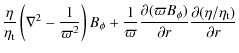
In Babcock-Leighton (BL) flux-transport dynamo models, the poloidal
field owes its origin to the tilt of magnetic loops emerging at the
solar surface. Thus, the source has to be confined to a thin layer just
below the surface and since the process is fundamentally non-local, the
source term depends on the variation of ![]() at the base of the convection zone (CZ). The expression is
at the base of the convection zone (CZ). The expression is
| |
= | ![$\displaystyle \frac{1}{2}\left[1+{\rm erf}\left(\frac{r-r_{2}}{d_{2}}\right)\right]\left[ 1-{\rm erf}\left(\frac{r-1}{d_{2}}\right)\right]$](/articles/aa/full_html/2010/01/aa13103-09/img81.png)
|
|
![$\displaystyle \times\left[1+\left({\frac{B_{\phi}(r_{\rm c},\theta,t)}{B_{0}}}\right)^{2}\right]^{-1}\cos\theta \sin\theta B_{\phi}(r_{\rm c},\theta,t)$](/articles/aa/full_html/2010/01/aa13103-09/img82.png)
|
where r2=0.95, d2=0.01,
In these BL flux-transport dynamo models, meridional
circulation is used to link the two sources of the magnetic
field namely the base of the CZ and the solar surface. The
structure of the meridional circulations in the Sun is less
constrained than the internal differential rotation, as they
possess slower flows that are difficult to detect
helioseismically. The nature of these flows in other stars is
even less constrained. It is generally believed that in the Sun,
the meridional circulations are likely to be composed largely of a
single cell in each hemisphere, and recent solar simulations
(Miesch et al. 2008) find such single-celled structures when the
global-scale flows are averaged over long intervals but multi-cellular profiles can also be realized.
In more rapidly rotating suns, 3-D models presently indicate that the
circulations are likely to be multi-celled in both radius and
latitude (Ballot et al. 2007; Brown et al. 2008).
In the series of models discussed in Sect. 3 of this paper,
we restrict ourselves to Babcock-Leighton flux-transport models
that have a large single cell per hemisphere. We choose this
simple profile because it is widely used in the community,
although some studies have considered more complex profiles (Bonanno et al. 2005; Jouve & Brun 2007a).
We are deferring to Sect. 4.2 the analysis of complex multi-cellular profiles.
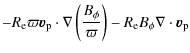
As in the Sun, the meridional circulations are
directed poleward at the surface and here they vanish at the
bottom boundary (r=0.6) and thus penetrate a little beneath the
tachocline into the radiative interior (cf. bottom panel of Fig. 1). To model the single cell meridional circulation
we consider a stream function with the following expression:
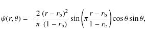
which gives, through the relation
| |
= | 
|
|
|
(10) |
| |
= | 
|
|
![$\displaystyle +\frac{r\pi}{1-r_{\rm b}}\frac{(r-r_{\rm b})}{(1-r_{\rm b})} \cos\left(\pi\frac{r-r_{\rm b}}{1-r_{\rm b}}\right)\Bigg]$](/articles/aa/full_html/2010/01/aa13103-09/img91.png)
|
|||
| (11) |
with
3 Flux transport models as a function of rotation rate
3.1 Previous results
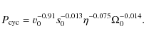
Jouve & Brun (2007a) have done a systematic study of the influence on the cycle period of the various parameters of Babcock-Leighton flux transport models. For the reference model possessing only one cell per hemisphere they confirm the results of Dikpati & Charbonneau (1999) that the cycle period is strongly dependent on the meridional circulation amplitude. A least square fit through the ensemble of models they computed leads to the following dependency:
We can thus expect that as we increase the rotation rate the cycle period will shorten if all the other parameters are kept constant but unfortunately not as fast as what is observed (Noyes et al. 1984; Saar 2002). However we may also expect the meridional circulation to depend on the rotation rate, and the sign of the variation of v0 with
3.2 Implementing results from 3D simulations of rapidly rotating stars in our mean field dynamo models
In order to get some physical insight on how the meridional circulation varies with the rotation rate we rely on recent 3-D numerical simulations of solar convection performed with the ASH code (Brun & Toomre 2002; Ballot et al. 2007; Brown et al. 2008). Indeed there are no reliable observations of the meridional circulation in stars except for the Sun near the surface. The theoretical work of Brown et al. (2008), that studies the influence of the rotation rate on solar like stars (i.e. with the same thickness for the convection zone as our current Sun), will provide the required scaling. In this work several 3-D purely hydrodynamical models have been computed at various rotation rates (from 1 to 10 times solar) and the redistribution of angular momentum, heat and energy assessed systematically to explain the differential rotation and meridional circulations achieved in the simulations. Figures 10 and 12 of Brown et al. (2008) are particularly relevant to our study and we have used the data from all the models reported in these figures plus more slowly rotating cases (i.e. with a rotation rate lower than the solar rate) that are currently being studied (Brown 2009).
Table 1:
Summary of the different cases studied and the values of ![]() and
and ![]() used in the 2D Babcock-Leighton models.
used in the 2D Babcock-Leighton models.
![\begin{figure}
\par\includegraphics[width=6.6cm,clip]{13103f2a.eps}\par\vspace*{...
...2mm}
\includegraphics[width=6.6cm,clip]{13103f2d.eps} \vspace{-3mm}
\end{figure}](/articles/aa/full_html/2010/01/aa13103-09/img108.png)
|
Figure 2:
Butterfly diagrams for cases G0.5, G1, G5 and G10. The top panel shows the time-latitude cut of the toroidal field at the base of the
convection zone and the bottom one represents the evolution of the radial field at the surface. Time is in years. The scale of the color
table is the same for all: between
|
| Open with DEXTER | |
We have thus scaled the meridional circulation by taking into account the way meridional circulation kinetic energy (MCKE)
is found to change with rotation in the published 3-D models of Brown et al. (2008).
We are confident that this scaling for MCKE still holds in the
magnetized version since recent 3-D models of dynamo action in rapidly
rotating suns find that the weak meridional circulations are
essentially unmodified by the strong magnetic fields that are generated
(Brown et al. 2009).
In contrast, the differential rotation appears to be substantially different
from that found in hydrodynamic cases, and its scaling with
rotation rate is sensitive to magnetic fields that are realized. We will thus not use the scaling
of
![]() with
with ![]() found in Brown et al. (2008) when we will vary the differential
rotation profile in our models but instead rely on observations (see Sect. 4.1 below).
found in Brown et al. (2008) when we will vary the differential
rotation profile in our models but instead rely on observations (see Sect. 4.1 below).
In Table 1, we list the solar-like mean field dynamo models that we have computed at various rotation rate along with
the associated Reynolds numbers ![]() and
and ![]() that we have used in our 2-D models. A quick look at the table already
reveals that the meridional circulation amplitude decreases with
rotation rate. This may come as a surprise as one could have expected
faster meridional flows as
that we have used in our 2-D models. A quick look at the table already
reveals that the meridional circulation amplitude decreases with
rotation rate. This may come as a surprise as one could have expected
faster meridional flows as ![]() is increased. However a careful study, via the longitudinal component
of the vorticity equation, of the maintenance of the meridional
circulation (which arises from small unbalance between large forces;
see for instance Miesch 2005; Brun & Rempel 2008), reveals that it
actually weakens with faster rotation rate.
It is thus likely given the strong negative dependency of
is increased. However a careful study, via the longitudinal component
of the vorticity equation, of the maintenance of the meridional
circulation (which arises from small unbalance between large forces;
see for instance Miesch 2005; Brun & Rempel 2008), reveals that it
actually weakens with faster rotation rate.
It is thus likely given the strong negative dependency of
![]() with v0
that
as we increase the rotation rate, the cycle period will increase rather
than decrease as observed. However it is not obvious to anticipate the
resulting field topology of the various models without actually
computing them.
with v0
that
as we increase the rotation rate, the cycle period will increase rather
than decrease as observed. However it is not obvious to anticipate the
resulting field topology of the various models without actually
computing them.
Incorporating the values of the dynamo numbers ![]() and
and ![]() for
the different stars in our flux-transport BL dynamo models enables us
to study the behaviour of the mean magnetic field in such stars in the
framework of mean-field theory. All the dynamo models we have studied
give cyclic behaviours with different periods and different intensity
of the mean toroidal and poloidal magnetic fields.
We wish to stress that even though the naming scheme of the models
discussed in this paper is similar to that used in Brown et al. (2008), the models are distinct since the ones discussed in this work are 2-D not 3-D.
for
the different stars in our flux-transport BL dynamo models enables us
to study the behaviour of the mean magnetic field in such stars in the
framework of mean-field theory. All the dynamo models we have studied
give cyclic behaviours with different periods and different intensity
of the mean toroidal and poloidal magnetic fields.
We wish to stress that even though the naming scheme of the models
discussed in this paper is similar to that used in Brown et al. (2008), the models are distinct since the ones discussed in this work are 2-D not 3-D.
![\begin{figure}
\par\includegraphics[width=8.4cm,clip]{13103f3.eps} \vspace{-6mm}
\end{figure}](/articles/aa/full_html/2010/01/aa13103-09/img109.png)
|
Figure 3:
Representative solution of a BL model applied to a
rapidly rotating star. This is case G5, with a rotation rate |
| Open with DEXTER | |
Figure 2 gives examples of 4 different butterfly diagrams obtained for more or less rapidly rotating stars. This figure shows the evolution in time of the toroidal magnetic field at the bottom of the CZ and of the radial field at the top of the domain. We note that the behaviour of the field is very similar in all these models, except that the period is clearly varying as well as the intensity of the magnetic field (the scale of the color table is the same for all panels). Indeed, we note that the magnetic cycle period is increased when the rotation rate is increased. This is a direct consequence of the fact that the cycle period is almost inversely proportional to the amplitude of the meridional flow in BL models.
In order to illustrate the temporal evolution of the magnetic field in the meridional plane, we display in Fig. 3 a temporal sequence over one starspot cycle for model G5. The advection of the field by the single-celled meridional circulation is evident confirming that our dynamo model is dominated by advection and not by diffusion. We wish to stress here that our particular choice of advection-dominated regime is not the only possibility at hand to model the transport occurring in the solar convection zone and the manner that the models link the Babcock-Leighton surface source term to the deep tachocline. For instance Chatterjee et al. (2004), Käpylä et al. (2006), Yeates et al. (2008), Guerrero & Gouveia Dal Pino (2008) have studied how transporting the poloidal field from the surface to the tachocline via turbulent diffusion or turbulent pumping influence the butterfly diagram, the polarity of the field and the cycle period. We intend to look at these solutions in the near future.
Returning to Fig. 3 we also note that the poloidal field tends to be more
concentrated near the polar region in agreement with the stronger polar branch seen in the corresponding butterfly diagram.
Indeed in Fig. 2 we clearly note that the magnetic intensity is increased when the rotation rate is increased,
which is in agreement with the observations.
We finally also note on the poloidal field that the contrast between the polar intensity and the
intensity close to the equator is diminished when the rotation rate is increased.
3.3 Field topology and poloidal vs. toroidal field ratio
It is clear that the evolution of the field topology as a function of the rotation rate is of great importance. We are thus summarizing in Table 2 and on the curves of Fig. 4 how the field intensity and topology is changing with
Table 2: Starspot cycle period (in year), maximum of toroidal field (in 104 G) at the base of the CZ and ratio between poloidal and toroidal field for 10 different cases with various rotation rates.
![\begin{figure}
\par\hspace*{2mm}\includegraphics[width=6.8cm,clip]{13103f4a.ps}\...
...2mm}
\includegraphics[width=7cm,clip]{13103f4d.eps}
\vspace{-4mm}
\end{figure}](/articles/aa/full_html/2010/01/aa13103-09/img110.png)
|
Figure 4:
Top panel: variation of the magnetic cycle period wih respect to the amplitude of the MC and ( 2nd panel) to the rotation rate
for the cases G1 to G10. On the third panel
we display the variation of the maximum of toroidal field at the base
of the CZ for two series of models. The solid line corresponds to the
models G1 to G10 using the scaled
down meridional flow as a function of the rotation rate whereas the
dotted line corresponds to another set of models for which v0 was kept constant.
On the bottom panel, we show the ratio
|
| Open with DEXTER | |
More precisely on the first (top) panel of Fig. 4,
we recover the almost proportional relationship between the magnetic
cycle period and the inverse of the meridional flow amplitude. This
again shows the major impact of the meridional circulation in these
Babcock-Leighton dynamo models on the cycle period.
As stated in Brown et al. (2008),
the meridional circulation kinetic energy in 3-D hydrodynamical (HD)
models of rapidly rotating stars seems to scale as approximately
![]() ,
leading the averaged meridional flow amplitude to scale as
,
leading the averaged meridional flow amplitude to scale as
![]() .
Indeed, on the second panel of Fig. 4 where we show the cycle period plotted against the rotation rate of the star,
we naturally recover a scaling in
.
Indeed, on the second panel of Fig. 4 where we show the cycle period plotted against the rotation rate of the star,
we naturally recover a scaling in
![]() .
A star rotating at
.
A star rotating at
![]() for example would have a cycle period of about 26 years approximately
40.45=1.87 times
the period of 15.1 years of case G2 rotating at twice the solar rate.
for example would have a cycle period of about 26 years approximately
40.45=1.87 times
the period of 15.1 years of case G2 rotating at twice the solar rate.
More interestingly, if we now focus on the third and fourth (bottom) panels of Fig. 4, we note that the amplitude of the toroidal field possesses an almost linear
dependency on the rotation rate ![]() .
This property is due mainly to two effects: a) a larger
.
This property is due mainly to two effects: a) a larger ![]() -effect (via its dependence on the Reynolds number
-effect (via its dependence on the Reynolds number
![]() )
in more rapidly rotating stars and b) the fact that the reduction of
the meridional flow amplitude allows the poloidal field to be stretched
and amplified over a longer period of time
(see Nandy (2004) and Yeates et al. (2008) who are finding similar effects).
This is evident by comparing on the third panel of Fig. 4
the solid and dashed curves. The difference between the two curves is
the amplitude of
the meridional flow as a function of rotation rate that we kept
constant for the cases shown using dashed line (these models
were used to determine the least square fit of Eq. (12)). We
clearly see that both series of models lead to larger toroidal field as
we increase the rotation rate
but for the series with the scaled down meridional flow, the
strengthening of
)
in more rapidly rotating stars and b) the fact that the reduction of
the meridional flow amplitude allows the poloidal field to be stretched
and amplified over a longer period of time
(see Nandy (2004) and Yeates et al. (2008) who are finding similar effects).
This is evident by comparing on the third panel of Fig. 4
the solid and dashed curves. The difference between the two curves is
the amplitude of
the meridional flow as a function of rotation rate that we kept
constant for the cases shown using dashed line (these models
were used to determine the least square fit of Eq. (12)). We
clearly see that both series of models lead to larger toroidal field as
we increase the rotation rate
but for the series with the scaled down meridional flow, the
strengthening of ![]() is even higher. As a result, in our set of 2-D BL dynamo models the
poloidal to toroidal
field ratio is found to increase almost linearly with the rotation
period (inversely proportional to the rotation rate as seen on the last
panel of Fig. 4).
This is in reasonable agreement with the observations of rapidly rotating solar-like stars by Petit et al. (2008). However the scaling of
is even higher. As a result, in our set of 2-D BL dynamo models the
poloidal to toroidal
field ratio is found to increase almost linearly with the rotation
period (inversely proportional to the rotation rate as seen on the last
panel of Fig. 4).
This is in reasonable agreement with the observations of rapidly rotating solar-like stars by Petit et al. (2008). However the scaling of
![]() /
/
![]() found in recent 3-D MHD
simulations computed by Brown et al. (2009)
is not linear. Moreover, the observations indicate that the energy
stored in the large-scale toroidal
component of the magnetic field tends to dominate for rotation periods
lower than 12 days (corresponding approximately to a rotation rate of
twice the solar one). In our cases, the toroidal
field is always dominant, even for the case with
found in recent 3-D MHD
simulations computed by Brown et al. (2009)
is not linear. Moreover, the observations indicate that the energy
stored in the large-scale toroidal
component of the magnetic field tends to dominate for rotation periods
lower than 12 days (corresponding approximately to a rotation rate of
twice the solar one). In our cases, the toroidal
field is always dominant, even for the case with
![]() where the poloidal field hardly reaches
where the poloidal field hardly reaches ![]() of the toroidal field.
of the toroidal field.
This discrepancy could be due to the fact that the values quoted in Petit et al. (2008) are related to observationally detectable fields, i.e. to surface fields; whereas the values we quote in this work are related to the magnetic fields in the whole convection zone. If the strong toroidal fields stored at the base of the convection zone are not able to reach the solar surface (as it is the case under certain conditions, see Jouve & Brun 2009 for more details), the surface measurements could underestimate the amount of magnetic energy stored in the toroidal fields in the whole stellar convective envelope.
4 Varying the model parameters
From the above set of models it is clear that just increasing the rotation rate of the model and/or implementing a scaled meridional circulation amplitude is not sufficient to reproduce the fast (close to linear) reduction of the stellar cycle period with the rotation rate. We thus wish in this section to modify all the other parameters in order to find the best set of models to reproduce the observations.
The first easiest modification is to change the value of the diffusivity or of the constant s0 used in the model. From the least square fit shown in Eq. (12)
the weak dependency of
![]() on
on ![]() or s0
indicates that it is unlikely that such a modification will be able to
reproduce the observations. We thus need to look for more sophisticated
solutions. In order to make the discussion easy to follow and to reduce
the number of models considered we will now limit our study to cases
rotating at five times the solar rate. Of course our results
are easily transposable to other rotation rates.
or s0
indicates that it is unlikely that such a modification will be able to
reproduce the observations. We thus need to look for more sophisticated
solutions. In order to make the discussion easy to follow and to reduce
the number of models considered we will now limit our study to cases
rotating at five times the solar rate. Of course our results
are easily transposable to other rotation rates.
4.1 Modifying the differential rotation profile
As discussed in the introduction it is clear that in low mass stars
the differential rotation is expected to change with the rotation rate.
Given the key role played
by the ![]() -effect
in mean field dynamo, we propose to compute a new model at 5 times the
solar rate with a modified differential rotation, namely case G5om. But
what scaling of
-effect
in mean field dynamo, we propose to compute a new model at 5 times the
solar rate with a modified differential rotation, namely case G5om. But
what scaling of
![]() with
with ![]() should we use?
In their 3-D hydrodynamic models, Brown et al. (2008) find a scaling of
should we use?
In their 3-D hydrodynamic models, Brown et al. (2008) find a scaling of
![]() .
However due to the nonlinear feed back of the Lorentz force on the mean
longitudinal flow, this scaling is not recovered in the MHD models
computed in Brown et al. (2009). We thus choose here not to use the theoretical scaling for
.
However due to the nonlinear feed back of the Lorentz force on the mean
longitudinal flow, this scaling is not recovered in the MHD models
computed in Brown et al. (2009). We thus choose here not to use the theoretical scaling for
![]() of Brown et al. (2008)
since it is somewhat uncertain and depends on whether or not dynamo
action is realized in the simulations.
The observational situation is not clearer with either a weak scaling
close to zero (i.e. the differential rotation does not vary with the
rotation rate; Barnes et al. 2005) or strong scaling as in Donahue et al. (1996). Given the current debate going on among the observers on the exact variation of
of Brown et al. (2008)
since it is somewhat uncertain and depends on whether or not dynamo
action is realized in the simulations.
The observational situation is not clearer with either a weak scaling
close to zero (i.e. the differential rotation does not vary with the
rotation rate; Barnes et al. 2005) or strong scaling as in Donahue et al. (1996). Given the current debate going on among the observers on the exact variation of
![]() with
with ![]() we have some freedom in the choice of our variation. We choose here to follow the scaling proposed by Donahue et al. (1996), i.e.
we have some freedom in the choice of our variation. We choose here to follow the scaling proposed by Donahue et al. (1996), i.e.
![]() since it is the most extreme variation found among the observers and as
a
consequence it will maximize the effect of varying the differential
rotation profile. The new differential rotation profile is shown on the
top panel of Fig. 5 and is directly comparable with the one shown on the top panel of Fig. 1.
We also display on the bottom panel of Fig. 5 the butterfly diagram for this new model G5om rotating at 5 times the solar rate with increased
since it is the most extreme variation found among the observers and as
a
consequence it will maximize the effect of varying the differential
rotation profile. The new differential rotation profile is shown on the
top panel of Fig. 5 and is directly comparable with the one shown on the top panel of Fig. 1.
We also display on the bottom panel of Fig. 5 the butterfly diagram for this new model G5om rotating at 5 times the solar rate with increased
![]() .
.
![\begin{figure}
\par\includegraphics[width=7cm,clip]{13103f5a.ps}\par\vspace*{2mm}
\includegraphics[width=7.5cm,clip]{13103f5b.ps}
\end{figure}](/articles/aa/full_html/2010/01/aa13103-09/img119.png)
|
Figure 5:
Top panel: new differential rotation used in the model G5om zoomed on the portion between r=0.6 and r=0.8. For that case
|
| Open with DEXTER | |
We see that the cycle period is almost not affected by the increase of
the latitudinal shear when comparing the butterfly diagram of Fig. 5 with the third panel of Fig. 2.
This confirms that the ![]() -effect
plays little role in setting the cycle period in BL dynamo models.
On the contrary the ratio between Bpol and Btor is changed. Indeed, for
this case, we go from a Bpol to Btor ratio of 0.05 in the standard case
G5 to a ratio of 0.019 in G5om. We thus proceeded in this case to a
significant increase of the toroidal component of the magnetic field,
keeping the value for the poloidal field approximately the same. This
is due to the fact that this new class of models is generating stronger
Btor as can be expected with a larger shear. A precise observation of
this ratio may thus be of utility to put constraints on stellar
internal differential rotation.
-effect
plays little role in setting the cycle period in BL dynamo models.
On the contrary the ratio between Bpol and Btor is changed. Indeed, for
this case, we go from a Bpol to Btor ratio of 0.05 in the standard case
G5 to a ratio of 0.019 in G5om. We thus proceeded in this case to a
significant increase of the toroidal component of the magnetic field,
keeping the value for the poloidal field approximately the same. This
is due to the fact that this new class of models is generating stronger
Btor as can be expected with a larger shear. A precise observation of
this ratio may thus be of utility to put constraints on stellar
internal differential rotation.
With a larger latitudinal shear it is expected that the tachocline at
the base of the stellar convection zone will also be modified. The
tachocline is
the transition region between the differentially rotating convective
envelope of low mass star and their supposedly uniformly rotating
radiative interior. How
the tachocline thickness is varying with the rotation rate and the
differential rotation of the star is not easy to determine. Based on
the
tachocline model of Spiegel & Zahn (1992) and the observations of
Donahue et al. (1996) for the dependency of
![]() with
with ![]() ,
Brun et al. (1999) have shown that the tachocline thickness for a younger more rapidly
rotating Sun could be thicker. They find a scaling for
,
Brun et al. (1999) have shown that the tachocline thickness for a younger more rapidly
rotating Sun could be thicker. They find a scaling for
![]() when taking into account all the dependencies. We have thus computed a
new model G5omt,
with both a larger tachocline (about twice as large in this case than
in case G5om, following the scaling law quoted above) and stronger
differential rotation (identical to case G5om shown on Fig. 5, with a
when taking into account all the dependencies. We have thus computed a
new model G5omt,
with both a larger tachocline (about twice as large in this case than
in case G5om, following the scaling law quoted above) and stronger
differential rotation (identical to case G5om shown on Fig. 5, with a
![]() about three times the solar one). The result in term of the cycle
period is again difficult to distinguish from the standard G5 model,
that had only
about three times the solar one). The result in term of the cycle
period is again difficult to distinguish from the standard G5 model,
that had only
![]() and the meridional circulation amplitude changed. This confirms that the
tachocline plays almost no role in Babcock-Leighton dynamo models in setting the cycle period.
On the contrary the ratio
and the meridional circulation amplitude changed. This confirms that the
tachocline plays almost no role in Babcock-Leighton dynamo models in setting the cycle period.
On the contrary the ratio
![]() /
/
![]() is modified being intermediate between the cases G5 and G5om. The value
of the ratio is now of about 0.02, very close to the case where the
differential rotation was increased, but with a slight reduction of the
toroidal component, due to the softer transition (i.e. thicker
tachocline). In summary neither models G5om nor G5omt possess a
cycle period in agreement with the observations and we thus need to
modify another physical ingredient.
is modified being intermediate between the cases G5 and G5om. The value
of the ratio is now of about 0.02, very close to the case where the
differential rotation was increased, but with a slight reduction of the
toroidal component, due to the softer transition (i.e. thicker
tachocline). In summary neither models G5om nor G5omt possess a
cycle period in agreement with the observations and we thus need to
modify another physical ingredient.
![\begin{figure}
\par\includegraphics[width=7cm,clip]{13103f6.ps}
\end{figure}](/articles/aa/full_html/2010/01/aa13103-09/img121.png)
|
Figure 6: Multicellular stream function for the case rotating at 5 times the solar rate G5mc20. Two cells with latitude have been used, with the first poleward cell near the equator closing at 20 deg of latitude. On the left panel we show the streamfunction and on the right panel the latitudinal velocity at 3 depths. |
| Open with DEXTER | |
In the standard Babcock-Leighton model we are thus left with two possibilities if we want to reconcile the models and the observations: modifying the profile of meridional circulation or introducing the effects of a faster rotation rate on the surface source term. Indeed, for example it has been shown by D'Silva & Choudhuri (1993) that the Coriolis force could strongly act on the tilt angle of emerging active regions, thus modifying the source term for poloidal field. This feature will have to be checked in future works, with the help of 3-D MHD models such as the ones of Jouve & Brun (2009). For this work, since the dependence of the cycle period on the amplitude of the meridional flow is very strong, we decide to focus on the first solution: modifying the MC profile.
4.2 Varying the number of meridional circulation cells
The strong relation between the meridional circulation speed and the cycle activity is an indication that shortening the advection path may result in shorter cycle period. Dikpati et al. (2004), Bonanno et al. (2005) and Jouve & Brun (2007a) have studied in detail the influence of various meridional circulation profiles on the butterfly diagram and other large scale magnetic properties of the Sun.
In particular Jouve & Brun (2007a) have shown that adding cells in radius slows down the cycle whereas as the two other groups also showed, adding cells in latitude accelerates it. If one seeks to shorten the cycle length as it is the case in this study, only adding cells in latitude will have the expected impact. We have thus computed a new set of simulations, rotating at five times the solar rate in which we have only modified the meridional circulation in latitude (leaving all the other parameters the same as in case G5) by considering two cells in latitude per hemisphere with various extension instead of just one cell.
Following the 3-D results of Brown et al. (2008)
and particularly Fig. 11 of their article, we choose to introduce
a meridional circulation with a counterclockwise cell at lower
latitudes and a clockwise cell at higher latitudes in the Northern
hemisphere, this profile being antisymmetric with respect to the
equator. Since uncertainties are significant concerning
the extension of the low-latitude meridional cell, we have computed
several models at 5 times the solar rate including a low-latitude cell
extending to
![]() ,
,
![]() ,
,
![]() and
and
![]() ,
named respectively G5mc45, G5mc40, G5mc30 and G5mc20. For the sake of
clarity we have decided to illustrate and discuss in length in this
section only one case, namely case G5mc20, the model with the less
extended lower meridional circulation cell. The meridional circulation
profile for that case is shown in Fig. 6
for illustration. In all models we have set the latitudinal velocity
such that it has the same maximal amplitude in the two counter-cells
which correspond to that in the case with one single cell (i.e. case
G5) keeping all the other parameters the same.
,
named respectively G5mc45, G5mc40, G5mc30 and G5mc20. For the sake of
clarity we have decided to illustrate and discuss in length in this
section only one case, namely case G5mc20, the model with the less
extended lower meridional circulation cell. The meridional circulation
profile for that case is shown in Fig. 6
for illustration. In all models we have set the latitudinal velocity
such that it has the same maximal amplitude in the two counter-cells
which correspond to that in the case with one single cell (i.e. case
G5) keeping all the other parameters the same.
![\begin{figure}
\par\includegraphics[width=7.5cm,clip]{13103f7.ps} \vspace{-4mm}
\end{figure}](/articles/aa/full_html/2010/01/aa13103-09/img126.png)
|
Figure 7: Butterfly diagram of the case G5mc20, rotating at 5 times the solar rotation rate and possessing a multicellular meridional flow as shown in Fig. 6. |
| Open with DEXTER | |
When comparing the various multi-cellular stellar dynamo simulations,
we find that the scaling of the cycle period with the extension of the
low-latitude cell is almost linear, the starspot cycle period being
respectively of 9.9, 9.2, 7.4 and 5.2 years for those different models.
This is mainly due to the fact that the advection path is reduced by
the presence of counter-cells and will shorten the distance each
component of the magnetic field has to travel before reaching the
region where it will be turned into the other component. According to
the previous studies and scaling laws of Noyes et al. (1984), Saar & Brandenburg (1999), Charbonneau & Saar (2001) and Saar (2002),
the cycle period for a star rotating at 5 times the rotation rate
should be around 3 years. We are getting very close to this value
with a low-latitude cell extending to
![]() in latitude as in case G5mc20. We now focus on butterfly diagram and
the evolution of the field in the meridional plane of this model, as
shown in Figs. 7 and 8.
in latitude as in case G5mc20. We now focus on butterfly diagram and
the evolution of the field in the meridional plane of this model, as
shown in Figs. 7 and 8.
On the butterfly diagram shown in Fig. 7,
we clearly see that we have significantly reduced the length of the
activity (starspot) cycle: the period is now 5.2 yr instead of
20.8 yr. The cyclic activity tends now to be more concentrated at
low latitudes. The temporal evolution of the field seems to be less
steady if we consider the variations of intensity which appear from one
cycle to the next, visible on the butterfly diagram through changes in
color between the different activity cycles. The radial field appears
to be even more busy, exhibiting a periodic but yet complex pattern at
low latitudes. We moreover note
that above
![]() ,
the cyclic activity is lost and we are left with some regions where the magnetic field evolves much more slowly than the
time scale of the main cycle.
,
the cyclic activity is lost and we are left with some regions where the magnetic field evolves much more slowly than the
time scale of the main cycle.
![\begin{figure}
\par\includegraphics[width=8cm]{13103f8.eps}
\end{figure}](/articles/aa/full_html/2010/01/aa13103-09/img128.png)
|
Figure 8: Same as Fig. 3 but for the case G5mc20 rotating at 5 times the rotation rate and possessing a multicellular meridional circulation as shown in Fig. 6. The evolution is shown over a temporal interval of 5.2 years corresponding to half a magnetic cycle or one starspot cycle. |
| Open with DEXTER | |
Looking at Fig. 8 will help us to have more insight on how the field is organized in the convective envelope and how it is advected by the new meridional circulation. Again, we clearly see that the evolution of the field is much more complicated than in the standard case. We can still follow the evolution of each component of the field on the various panels of the figure. Indeed we can distinguish the effect of the low-latitude cell which advects the newly generated poloidal field (counterclockwise on the first panel) downwards while the toroidal field of the previous cycle (positive i.e. represented by reddish colours) is being advected at the base of the convection zone to reach the equator and replace the toroidal field of the previous cycle at the end of the starspot cycle (last panel). We note, in agreement with the butterfly diagram, that the advection at higher latitudes is much slower and as a consequence we do not clearly see any imprint of the activity cycle in the polar regions. This is due to the fact that the same amplitude of the flow is introduced for both cells and that the distance traveled by the field at low latitudes is much shorter, thus leading to a difference in the time-scale for the advection of the magnetic field in the two cells. We also wish to reemphasize that we did not introduce multi cells in radius since Jouve & Brun (2007a) showed that it results in a slowing down of the cycle period rather than a speeding up as required in this study for fastly rotating stars. In summary adding cell in latitude clearly helps shortening the cycle for fastly rotating stars. For the stars rotating slower than the Sun it may be necessary to add cells in radius if one wants to increase the cycle. Indeed 3-D models indicate that slower the star rotates faster its meridional circulation is and thus shorter its cyclic period will be as demonstrated by the butterfly diagram shown on the top panel of Fig. 2 for case G0.5.
5 Summary and conclusions
The idea of this work was to better understand stellar magnetism, using
both 2-D and 3-D calculations. To do so, we have introduced into
Babcock-Leighton (B-L) flux transport dynamo models, results from 3-D
global hydrodynamical simulations by Brown et al. (2008).
To be more specific we have used these simulations to determine the
variation of the amplitude of the meridional circulation with rotation
rate and complemented our study with observations of the variation of
the angular velocity contrast
![]() with rotation rate. Using these scaling laws we have built a series of 2-D mean field stellar dynamo models in which
we have modified in turn the rotation rate, the amplitude of the meridional circulation and of the angular velocity gradient.
This has allowed us to test the validity of this type of models on solar-like stars with faster rotations and intense magnetism.
with rotation rate. Using these scaling laws we have built a series of 2-D mean field stellar dynamo models in which
we have modified in turn the rotation rate, the amplitude of the meridional circulation and of the angular velocity gradient.
This has allowed us to test the validity of this type of models on solar-like stars with faster rotations and intense magnetism.
Our study shows that an increase in the rotation rate leads to a larger ![]() -effect which in turn modifies the ratio between
poloidal and toroidal fields with a trend similar to that found observationally in a
small sample of rapidly rotating suns (Petit et al. 2008).
Other authors have also studied such trends using solar mean field B-L
flux transport dynamo models (see for instance Charbonneau & Saar 2001; Dikpati et al. 2001; Nandy & Martens 2007).
They also find that the toroidal field grows in amplitude with the
star's rotation rate.
The difference between our work and previous studies comes from the
choice made in varying the meridional circulation amplitude with
rotation rate. In 3-D global calculations an increase of the rotation
rate leads to a decrease in the meridional flow amplitude whereas in
previous studies the opposite was assumed since such knowledge was not
yet available. Given that the cycle period in advection-dominated B-L
dynamo models is almost inversely proportional to the intensity of the
meridional circulation, we find that our models predict slower magnetic
cycles for more rapidly rotating stars. This is not consistent with the
observational data collected at Mount Wilson since the 1960's (e.g.
Noyes et al. 1984; Baliunas et al. 1995).
It thus seems difficult to reconcile advection-dominated B-L models
widely used in the solar dynamo community with stellar activity
observations if we use scaling laws relating
rotation rates and meridional flow amplitudes given by consistent 3-D
models. Of course the systematic observation of the meridional
circulation realized in solar-like stars rotating at various rotation
rate would
be of great use and could solve the apparent discrepancy if we indeed
found that such flows are not so sensitive to the rotation rate.
Unfortunately such observations are not yet available. Hopefully with
the Corot and Kepler satellites now in orbit this situation may change
in the near future.
-effect which in turn modifies the ratio between
poloidal and toroidal fields with a trend similar to that found observationally in a
small sample of rapidly rotating suns (Petit et al. 2008).
Other authors have also studied such trends using solar mean field B-L
flux transport dynamo models (see for instance Charbonneau & Saar 2001; Dikpati et al. 2001; Nandy & Martens 2007).
They also find that the toroidal field grows in amplitude with the
star's rotation rate.
The difference between our work and previous studies comes from the
choice made in varying the meridional circulation amplitude with
rotation rate. In 3-D global calculations an increase of the rotation
rate leads to a decrease in the meridional flow amplitude whereas in
previous studies the opposite was assumed since such knowledge was not
yet available. Given that the cycle period in advection-dominated B-L
dynamo models is almost inversely proportional to the intensity of the
meridional circulation, we find that our models predict slower magnetic
cycles for more rapidly rotating stars. This is not consistent with the
observational data collected at Mount Wilson since the 1960's (e.g.
Noyes et al. 1984; Baliunas et al. 1995).
It thus seems difficult to reconcile advection-dominated B-L models
widely used in the solar dynamo community with stellar activity
observations if we use scaling laws relating
rotation rates and meridional flow amplitudes given by consistent 3-D
models. Of course the systematic observation of the meridional
circulation realized in solar-like stars rotating at various rotation
rate would
be of great use and could solve the apparent discrepancy if we indeed
found that such flows are not so sensitive to the rotation rate.
Unfortunately such observations are not yet available. Hopefully with
the Corot and Kepler satellites now in orbit this situation may change
in the near future.
We have thus tried to investigate ways to improve the agreement
between 2-D models and observations in refining our calculations. A
least-square fit on the various parameters of the standard model
shows that we cannot rely on a modifications of ![]() ,
s0 and
,
s0 and ![]() to act on the cycle period, as the latter is almost completely
determined by the amplitude of the meridional flow (see Eq. (12)).
We thus computed more sophisticated models where the differential
rotation and meridional circulation profiles were modified.
to act on the cycle period, as the latter is almost completely
determined by the amplitude of the meridional flow (see Eq. (12)).
We thus computed more sophisticated models where the differential
rotation and meridional circulation profiles were modified.
First, we computed a model at 5 times the solar rotation rate
where the modified contrast
in the angular velocity was taken into account. Some uncertainties both
from an observational or a theoretical standpoint still exist
concerning the scaling between
![]() and
and ![]() but we find that the effect on the cycle
period is negligible, even when we consider the most extreme
observation of the variation of the differential rotation contrast with
rotation rate (Donahue et al. 1996).
Modifying the tachocline thickness as a function of rotation rate according to the scaling law of Brun et al. (1999)
does not help to improve the relationship between the rotation rate of
the star and the cycle period either. We show that the main impact of a
modification
of the profile of differential rotation is to decrease the percentage
of the poloidal component in the total magnetic field again because of
the increased efficiency of the
source for toroidal field: the
but we find that the effect on the cycle
period is negligible, even when we consider the most extreme
observation of the variation of the differential rotation contrast with
rotation rate (Donahue et al. 1996).
Modifying the tachocline thickness as a function of rotation rate according to the scaling law of Brun et al. (1999)
does not help to improve the relationship between the rotation rate of
the star and the cycle period either. We show that the main impact of a
modification
of the profile of differential rotation is to decrease the percentage
of the poloidal component in the total magnetic field again because of
the increased efficiency of the
source for toroidal field: the ![]() -effect.
The modification of the source term for poloidal field (decay of active
regions in Babcock-Leighton models and the kinetic
helicity of the flow in
-effect.
The modification of the source term for poloidal field (decay of active
regions in Babcock-Leighton models and the kinetic
helicity of the flow in ![]() -
-![]() models) due to an increase of the rotation rate still needs to be
addressed to study the evolution of the poloidal to toroidal field
ratio in those refined cases.
models) due to an increase of the rotation rate still needs to be
addressed to study the evolution of the poloidal to toroidal field
ratio in those refined cases.
Given the strong dependency of the magnetic cycle period on the
meridional circulation and the fact that 3-D models exhibit
multicellular patterns of the flow in latitude, it is
reasonable to think that modifying the profile of the MC according to
3-D models may help to get closer to the observational data. Indeed, we
show that adding a counter cell in latitude
which extends until about
![]() in both hemispheres reduces drastically the cycle period. We find a
quasi-linear relationship between the extension of the counter cell and
the cycle
period, which is very promising to reconcile Babcock-Leighton models
with observations of stellar activity. Another solution could be to
change the way poloidal magnetic fields are transported from the
surface down to the tachocline. In Yeates et al. (2008)
the transport is dominated by diffusion to link the distant magnetic
field generation regions. In their case the cycle period seems less
sensitive to the meridional flow amplitude and profile assumed and
depends more on the diffusion profile. Guerrero &
Gouveia Dal Pino (2008)
have introduced in Babcock-Leighton dynamo equations an extra term
representing the pumping of magnetic fields due to turbulent convection
(inspired by the work of Käpylä et al. 2006). This new process leads to vertical and
horizontal transport of the fields. Their model seems to show a significant decrease
of the cycle period dependency on the meridional flow amplitude (from
v0-0.9 to
v0-0.12, although only a shallow
meridional flow is considered, which may influence the scaling law) and
that the turbulent pumping is now responsible for regulating the cyclic
activity. Reintroducing the meridional flow amplitude scalings deduced
from 3-D calculations in this type of models would thus have much less
impact on the cycle period. The changes in the pumping coefficients
with respect to the rotation rate would have to be investigated to see
if some of the observations of stellar magnetic activity could be
recovered.
in both hemispheres reduces drastically the cycle period. We find a
quasi-linear relationship between the extension of the counter cell and
the cycle
period, which is very promising to reconcile Babcock-Leighton models
with observations of stellar activity. Another solution could be to
change the way poloidal magnetic fields are transported from the
surface down to the tachocline. In Yeates et al. (2008)
the transport is dominated by diffusion to link the distant magnetic
field generation regions. In their case the cycle period seems less
sensitive to the meridional flow amplitude and profile assumed and
depends more on the diffusion profile. Guerrero &
Gouveia Dal Pino (2008)
have introduced in Babcock-Leighton dynamo equations an extra term
representing the pumping of magnetic fields due to turbulent convection
(inspired by the work of Käpylä et al. 2006). This new process leads to vertical and
horizontal transport of the fields. Their model seems to show a significant decrease
of the cycle period dependency on the meridional flow amplitude (from
v0-0.9 to
v0-0.12, although only a shallow
meridional flow is considered, which may influence the scaling law) and
that the turbulent pumping is now responsible for regulating the cyclic
activity. Reintroducing the meridional flow amplitude scalings deduced
from 3-D calculations in this type of models would thus have much less
impact on the cycle period. The changes in the pumping coefficients
with respect to the rotation rate would have to be investigated to see
if some of the observations of stellar magnetic activity could be
recovered.
In conclusion, advection-dominated Babcock-Leighton flux-transport models may offer insights into the dynamo action occurring within the convection zones of solar-type stars. However, it is necessary to make serious modifications to these models if we wish to reconcile their predictions with observations of real stellar magnetism.
AcknowledgementsWe acknowledge funding from the European Community via the ERC-StG grant STARS2 207430 (www.stars2.eu). We are thankful to T. Emonet & P. Charbonneau for the original version of the STELEM code, to M. Browning for fruitful discussions on stellar magnetism and rotation and to the organizers of the dynamo program at KITP in Santa Barbara in 2008 where this work was initiated. We are also thankful to the anonymous referee whose comments helped improve the quality of the paper. B.P. Brown wishes to acknowledge fundings through the NASA GSRP program by award number NNG05GN08H.
References
- Babcock, H. W. 1961, ApJ, 133, 572 [Google Scholar]
- Baliunas, S. L., Donahue, R. A., Soon, W. H., et al. 1995, ApJ, 438, 269 [NASA ADS] [CrossRef] [Google Scholar]
- Baliunas, S. L., Nesme-Ribes, E., Sokoloff, D., & Soon, W. H. 1996, ApJ, 460, 848 [NASA ADS] [CrossRef] [Google Scholar]
- Ballot, J., Brun, A. S., & Turck-Chièze, S. 2007, ApJ, 669, 1190 [Google Scholar]
- Barnes, J. R., Cameron, A. C., Donati, J.-F., et al. 2005, MNRAS, 357, L1 [NASA ADS] [CrossRef] [MathSciNet] [Google Scholar]
- Bonanno, A., Elstner, D., Belvedere, G., & Rüdiger, G. 2005, Astron. Nachr., 326, 170 [NASA ADS] [CrossRef] [Google Scholar]
- Brown, B. P. 2009, Ph.D. Thesis, University of Colorado [Google Scholar]
- Brown, B. P., Browning, M. K., Brun, A. S., Miesch, M. S., & Toomre, J. 2008, ApJ, 689, 1354 [CrossRef] [Google Scholar]
- Brown, B. P., Browning, M. K., Brun, A. S., Miesch, M. S., & Toomre, J. 2009, ApJ, accepted [Google Scholar]
- Browning, M. K. 2008, ApJ, 676, 1262 [Google Scholar]
- Brun, A. S., & Toomre, J. 2002, ApJ, 570, 865 [NASA ADS] [CrossRef] [EDP Sciences] [Google Scholar]
- Brun, A. S., & Turck-Chièze, S., & Zahn, J.-P. 1999, ApJ, 525, 1032 [NASA ADS] [CrossRef] [Google Scholar]
- Brun, A. S., Miesch, M. S., & Toomre, J. 2004, ApJ, 614, 1073 [NASA ADS] [CrossRef] [Google Scholar]
- Cattaneo, F. 1999, ApJ, 515, L39 [NASA ADS] [CrossRef] [Google Scholar]
- Charbonneau, P. 2005, Living Rev. Sol. Phys., 2, 2 [NASA ADS] [Google Scholar]
- Charbonneau, P., & Saar, S. H. 2001, in Magnetic Fields across the H-R diagram, ed. G. Mathys, S. K. Solanki, & D. T. Wickamasinghe, ASP Conf. Ser., 248, 189 [Google Scholar]
- Chatterjee, P., Nandy, D., & Choudhuri, A. R. 2004, A&A, 427, 1019 [Google Scholar]
- Clune, T. L., et al. 1999, Parallel Comput., 25, 361 [CrossRef] [Google Scholar]
- D'Silva, S., & Choudhuri, A. R. 1993, A&A, 272, 621 [Google Scholar]
- Dikpati, M., & Charbonneau, P. 1999, ApJ, 518, 508 [NASA ADS] [CrossRef] [Google Scholar]
- Dikpati, M., Cally, P. S., & Gilman, P. A. 2004, ApJ, 610, 597 [NASA ADS] [CrossRef] [Google Scholar]
- Dikpati, M., Saar, S. H., Brummell, N., & Charbonneau, P. 2001, in Magnetic fields across the H-R diagram, ed. G. Mathys, S. K. Solanki, & D. T. Wickramasinghe, ASP Conf. Ser., 248, 235 [Google Scholar]
- Donahue, R. A., Saar, S. H., & Baliunas, S. L. 1996, ApJ, 466, 384 [NASA ADS] [CrossRef] [Google Scholar]
- Donati, J.-F., Howarth, I. D., Jardine, M. M., et al. 2006, MNRAS, 370, 629 [NASA ADS] [CrossRef] [Google Scholar]
- Durney, B. R., & Latour, J. 1976, Geophys. Astrophys. Fluid dynamics, 9, 241 [Google Scholar]
- Fan, Y. 2008, ApJ, 676, 680 [NASA ADS] [CrossRef] [Google Scholar]
- Giampapa, M. 2005, in The Sun, solar analogs and the climate, Saas-Fee Advanced Course 34, ed. I. Rüedi, M. Güdel, & W. Schmutz (Berlin: Springer), 307 [Google Scholar]
- Guerrero, G., & de Gouveia Dal Pino, E. 2008, A&A, 485, 267 [Google Scholar]
- Hempelmann, A., Schmitt, J. H. M. M., Schultz, M., Rüdiger, G., & Stepien, K. 1995, A&A, 294, 515 [Google Scholar]
- Käpylä, P. J., Korpi, M. J., & Tuominen, I. 2006, Astron. Nach., 327, 884 [Google Scholar]
- Knobloch, E., Rosner, R., & Weiss, N. O. 1981, MNRAS, 197, 45 [NASA ADS] [Google Scholar]
- Kosovichev, A. G., & Stenflo, J. O. 2008, ApJ, 688, L115 [NASA ADS] [CrossRef] [Google Scholar]
- Krause, F., & Raedler, K. H. 1980, Mean-field magnetohydrodynamics and dynamo theory (Oxford Pergamon Press) [Google Scholar]
- Küker, M., & Rüdiger, G. 2008, J. Phys. Conf. Ser., 118, 012029 [NASA ADS] [CrossRef] [Google Scholar]
- Jouve, L., & Brun, A. S. 2007a, A&A, 474, 239 [Google Scholar]
- Jouve, L., & Brun, A. S. 2007b, Astron. Nach., 328, 1104 [Google Scholar]
- Jouve, L., & Brun, A. S. 2009, ApJ, 701, 1300 [NASA ADS] [CrossRef] [Google Scholar]
- Jouve, L., Brun, A. S., Arlt, R., et al. 2008, A&A, 483, 949 [Google Scholar]
- Leighton, R. B. 1969, ApJ, 156, 1 [Google Scholar]
- Moffatt, H. K. 1978, Magnetic Field Generation in Electrically Conducting Fluids (Cambridge: Cambridge Univ. Press) [Google Scholar]
- Nandy, D. 2004, Sol. Phys., 224, 161 [NASA ADS] [CrossRef] [Google Scholar]
- Nandy, D., & Choudhuri, A. R. 2002, Science, 296, 1671 [NASA ADS] [CrossRef] [PubMed] [Google Scholar]
- Nandy, D., & Martens, P. C. H. 2007, AdSpR, 40, 7, 891 [Google Scholar]
- Noyes, R. W., Weiss, N. O., & Vaughan, A. H. 1984, ApJ, 287, 769 [NASA ADS] [CrossRef] [Google Scholar]
- Parker, E. N. 1993, ApJ, 408, 707 [Google Scholar]
- Petit, P., Dintrans, B., Solanki, S. K., et al. 2008, MNRAS, 388, 80 [NASA ADS] [CrossRef] [MathSciNet] [Google Scholar]
- Pizzolato, N., Maggio, A., Micela, G., Sciortino, S., & Ventura, P. 2003, A&A, 397, 147 [Google Scholar]
- Pouquet, A., Frisch, U., & Léorat, J. 1976, J. Fluid Mech., 77, 321 [NASA ADS] [CrossRef] [Google Scholar]
- Reiners, A., Basri, G., & Browning, M. 2009, ApJ, 692, 538 [NASA ADS] [CrossRef] [Google Scholar]
- Rempel, M. 2008, J. Phys. Conf. Ser., 118, 012032 [NASA ADS] [CrossRef] [Google Scholar]
- Saar, S. H., & Brandenburg, A. 1999, ApJ, 524, 295 [NASA ADS] [CrossRef] [Google Scholar]
- Saar, S. H. 2002, in the 11th Cool Stars: Stellar System and the Sun, ed. R. J. Garcia Lopez, R. Rebolo, & M. R. Zapatero, ASP Conf. Ser., 223, 292 [Google Scholar]
- Soon, W. H., Baliunas, S. L., & Zhang, Q. 1993, ApJ, 414, L33 [NASA ADS] [CrossRef] [Google Scholar]
- Thompson, M. J., Christensen-Dalsgaard, J., Miesch, M. S., & Toomre, J. 2003, ARA&A, 41, 599 [Google Scholar]
- Wang, Y.-M., Sheeley, N. R., Jr., & Nash, A. G. 1991, ApJ, 383, 431 [NASA ADS] [CrossRef] [Google Scholar]
- Wilmot-Smith, A. L., Nandy, D., Hornig, G., & Martens, P. C. H. 2006, ApJ, 652, 696 [NASA ADS] [CrossRef] [Google Scholar]
- Wilson, O. C. 1978, ApJ, 226, 379 [NASA ADS] [CrossRef] [Google Scholar]
- Yeates, A. R., Nandy, D., & Mackay, D. H. 2008, ApJ, 673, 544 [NASA ADS] [CrossRef] [Google Scholar]
All Tables
Table 1:
Summary of the different cases studied and the values of ![]() and
and ![]() used in the 2D Babcock-Leighton models.
used in the 2D Babcock-Leighton models.
Table 2: Starspot cycle period (in year), maximum of toroidal field (in 104 G) at the base of the CZ and ratio between poloidal and toroidal field for 10 different cases with various rotation rates.
All Figures
|
|
Figure 1: Top panel: differential rotation profile used in the models G0.25 to G10 discussed Sect. 3. We zoomed on the tachocline region between r=0.6 and r=0.8. Bottom panel: meridional circulation used in the models G0.25 to G10 discussed Sect. 3. Plain (dashed) lines indicate counterclockwise (clockwise) circulation. |
| Open with DEXTER | |
| In the text | |
|
|
Figure 2:
Butterfly diagrams for cases G0.5, G1, G5 and G10. The top panel shows the time-latitude cut of the toroidal field at the base of the
convection zone and the bottom one represents the evolution of the radial field at the surface. Time is in years. The scale of the color
table is the same for all: between
|
| Open with DEXTER | |
| In the text | |
|
|
Figure 3:
Representative solution of a BL model applied to a
rapidly rotating star. This is case G5, with a rotation rate |
| Open with DEXTER | |
| In the text | |
|
|
Figure 4:
Top panel: variation of the magnetic cycle period wih respect to the amplitude of the MC and ( 2nd panel) to the rotation rate
for the cases G1 to G10. On the third panel
we display the variation of the maximum of toroidal field at the base
of the CZ for two series of models. The solid line corresponds to the
models G1 to G10 using the scaled
down meridional flow as a function of the rotation rate whereas the
dotted line corresponds to another set of models for which v0 was kept constant.
On the bottom panel, we show the ratio
|
| Open with DEXTER | |
| In the text | |
|
|
Figure 5:
Top panel: new differential rotation used in the model G5om zoomed on the portion between r=0.6 and r=0.8. For that case
|
| Open with DEXTER | |
| In the text | |
|
|
Figure 6: Multicellular stream function for the case rotating at 5 times the solar rate G5mc20. Two cells with latitude have been used, with the first poleward cell near the equator closing at 20 deg of latitude. On the left panel we show the streamfunction and on the right panel the latitudinal velocity at 3 depths. |
| Open with DEXTER | |
| In the text | |
|
|
Figure 7: Butterfly diagram of the case G5mc20, rotating at 5 times the solar rotation rate and possessing a multicellular meridional flow as shown in Fig. 6. |
| Open with DEXTER | |
| In the text | |
|
|
Figure 8: Same as Fig. 3 but for the case G5mc20 rotating at 5 times the rotation rate and possessing a multicellular meridional circulation as shown in Fig. 6. The evolution is shown over a temporal interval of 5.2 years corresponding to half a magnetic cycle or one starspot cycle. |
| Open with DEXTER | |
| In the text | |
Copyright ESO 2010
Current usage metrics show cumulative count of Article Views (full-text article views including HTML views, PDF and ePub downloads, according to the available data) and Abstracts Views on Vision4Press platform.
Data correspond to usage on the plateform after 2015. The current usage metrics is available 48-96 hours after online publication and is updated daily on week days.
Initial download of the metrics may take a while.