| Issue |
A&A
Volume 509, January 2010
|
|
|---|---|---|
| Article Number | A73 | |
| Number of page(s) | 7 | |
| Section | Stellar structure and evolution | |
| DOI | https://doi.org/10.1051/0004-6361/200912749 | |
| Published online | 21 January 2010 | |
Non-radial oscillations in the red giant HR 7349 measured by CoRoT![[*]](/icons/foot_motif.png)
F. Carrier1 - J. De Ridder1 - F. Baudin2 - C. Barban3 - A. P. Hatzes4 - S. Hekker5,6,1 - T. Kallinger7,8 - A. Miglio9 - J. Montalbán9 - T. Morel9 - W. W. Weiss7 - M. Auvergne3 - A. Baglin3 - C. Catala3 - E. Michel3 - R. Samadi3
1 - Instituut voor Sterrenkunde, Katholieke Universiteit Leuven, Celestijnenlaan 200D,
3001 Leuven, Belgium
2 -
Institut d'Astrophysique Spatiale, Campus d'Orsay, 91405 Orsay, France
3 -
LESIA, UMR8109, Université Pierre et Marie Curie, Université Denis Diderot,
Observatoire de Paris, 92195 Meudon, France
4 -
Thüringer Landessternwarte, 07778 Tautenburg, Germany
5 -
University of Birmingham, School of Physics and Astronomy, Edgbaston, Birmingham B15 2TT, UK
6 -
Royal Observatory of Belgium, Ringlaan 3, 1180 Brussels, Belgium
7 -
Institute for Astronomy, University of Vienna, Türkenschanzstrasse 17, 1180 Vienna, Austria
8
- Department of Physics and Astronomy, University of British Columbia,
6224 Agricultural Road, Vancouver, BC V6T 1Z1, Canada
9 -
Institut d'Astrophysique et de Géophysique de l'Université de Liège, Allée du 6 Août 17, 4000 Liège, Belgium
Received 23 June 2009 / Accepted 7 October 2009
Abstract
Context. Convection in red giant stars excites resonant
acoustic waves whose frequencies depend on the sound speed inside the
star, which in turn depends on the properties of the stellar interior.
Therefore, asteroseismology is the most robust available method for
probing the internal structure of red giant stars.
Aims. Solar-like oscillations in the red giant HR 7349 are investigated.
Methods. Our study is based on a time series of 380 760
photometric measurements spread over 5 months obtained with the CoRoT
satellite. Mode parameters were estimated using maximum likelihood
estimation of the power spectrum.
Results. The power spectrum of the high-precision time series clearly exhibits several identifiable peaks between 19 and 40 ![]() Hz showing regularity with a mean large and small spacing of
Hz showing regularity with a mean large and small spacing of ![]() = 3.47
= 3.47 ![]() 0.12
0.12 ![]() Hz and
Hz and
![]() = 0.65
= 0.65 ![]() 0.10
0.10 ![]() Hz.
Nineteen individual modes are identified with amplitudes in the range
from 35 to 115 ppm. The mode damping time is estimated to be
14.7 +4.7-2.9 days.
Hz.
Nineteen individual modes are identified with amplitudes in the range
from 35 to 115 ppm. The mode damping time is estimated to be
14.7 +4.7-2.9 days.
Key words: stars: variables: general - stars: oscillations - stars: interiors - stars: individual: HR 7349
1 Introduction
The analysis of the oscillation spectrum provides an unrivaled method
for probing the stellar
internal structure because the frequencies of these oscillations depend
on the sound speed inside the
star, which in turn depends on the density, temperature, gas motion,
and other properties of the stellar
interior. High-precision spectrographs have acquired data yielding to a
rapidly growing list of solar-like oscillation detections
in main-sequence and giant stars (see e.g., Bedding & Kjeldsen 2007; Carrier et al. 2008).
In a few years, we have moved from ambiguous detections to firm measurements. Among these, only a few are
related to red giants, e.g., ![]() Hya, Frandsen et al.
(2002),
Hya, Frandsen et al.
(2002), ![]() Hya, De Ridder et al. (2006), and
Hya, De Ridder et al. (2006), and
![]() Hya, Barban et al. (2004).
The reason is that longer and almost uninterrupted time series are needed to characterize the oscillations in
red giants, because of longer oscillation periods than main-sequence stars, and long observing runs are
difficult to obtain using high-accuracy spectrographs.
Hya, Barban et al. (2004).
The reason is that longer and almost uninterrupted time series are needed to characterize the oscillations in
red giants, because of longer oscillation periods than main-sequence stars, and long observing runs are
difficult to obtain using high-accuracy spectrographs.
The CoRoT (COnvection ROtation and planetary Transits) satellite (Baglin 2006) is perfect for this purpose because it can provide these data for a large number of stars simultaneously. The CoRoT satellite continuously collects white-light high-precision photometric observations for 10 bright stars in the so-called seismofield, as well as 3-color photometry for thousands of relatively faint stars in the so-called exofield. The primary motivation for acquiring this second set of data is to detect planetary transits, but the data are also well suited to asteroseismic investigations. De Ridder et al. (2009) unambiguously detected long-lifetime non-radial oscillations in red giant stars in the exofield data of CoRoT, which is an important breakthrough for asteroseismology. Indeed, observations from either the ground or other satellites have been unable to confirm the existence of non-radial modes and determine a clear value of the mode lifetime. Hekker et al. (2009) presented a more detailed classification of the red giants observed by CoRoT.
![]() Hya (HD 181907) is a bright equatorial G8 giant star (V
= 5.82) that is an excellent target for asteroseismology. This star was
selected as a secondary target during the first long run of the
CoRoT mission.
In this paper, we thus report on photometric CoRoT observations of
Hya (HD 181907) is a bright equatorial G8 giant star (V
= 5.82) that is an excellent target for asteroseismology. This star was
selected as a secondary target during the first long run of the
CoRoT mission.
In this paper, we thus report on photometric CoRoT observations of
![]() Hya resulting in the detection and identification of
p-mode oscillations.
The non-asteroseismic observations are presented in Sect. 2, the
CoRoT data and frequency analysis in
Sects. 3 and 4, and the conclusions are given in
Sect. 5.
Hya resulting in the detection and identification of
p-mode oscillations.
The non-asteroseismic observations are presented in Sect. 2, the
CoRoT data and frequency analysis in
Sects. 3 and 4, and the conclusions are given in
Sect. 5.
2 Fundamental parameters
2.1 Effective temperature and chemical composition
We used the line analysis code MOOG, Kurucz models, and a
high-resolution FEROS spectrum obtained in June 2007 to carry out an
LTE abundance study of HR 7349.
The effective temperature and surface gravity were estimated from the
excitation and ionization equilibrium of a set of iron lines taken from
the line list of Hekker & Meléndez (2007). We obtain
![]() = 4790
= 4790 ![]() 80 K and [Fe/H] = -0.08
80 K and [Fe/H] = -0.08 ![]() 0.10 dex, while the abundance pattern of
the other elements with respect to Fe is solar within the errors.
The full results of the abundance analysis will be reported elsewhere (Morel et al.,
in preparation).
We also determined a photometric temperature given by the relation in Alonso et al. (1999) using
the dereddened color index (B-V) (see Sect. 2.2) and found 4704
0.10 dex, while the abundance pattern of
the other elements with respect to Fe is solar within the errors.
The full results of the abundance analysis will be reported elsewhere (Morel et al.,
in preparation).
We also determined a photometric temperature given by the relation in Alonso et al. (1999) using
the dereddened color index (B-V) (see Sect. 2.2) and found 4704 ![]() 110 K, which agrees with the spectroscopic value.
We finally adopt a weighted-mean temperature of 4760
110 K, which agrees with the spectroscopic value.
We finally adopt a weighted-mean temperature of 4760 ![]() 65 K.
65 K.
2.2 Luminosity
Even for such a bright star, the interstellar extinction in the direction of the Galactic center is not negligible. From the HIPPARCOS parallax2.3 Rotational velocity
We determined the rotational velocity of the star by means of a spectrum taken with the spectrograph CORALIE installed on the 1.2-m Swiss telescope, ESO La Silla, Chile. According to the calibration of Santos et al. (2002), we determined a2.4 Large spacing estimation
An estimation of the mass of HR 7349 may be obtained by matching evolutionary tracks to the
![]() error box in the HR diagram. However, in the red giant part of
the HR diagram, this determination is not robust at all. Assuming a mass of between 0.8 and 3
error box in the HR diagram. However, in the red giant part of
the HR diagram, this determination is not robust at all. Assuming a mass of between 0.8 and 3 ![]() and scaling from the solar case (Kjeldsen & Bedding 1995),
a large frequency spacing of 2.8-5.5
and scaling from the solar case (Kjeldsen & Bedding 1995),
a large frequency spacing of 2.8-5.5 ![]() Hz is expected.
Hz is expected.
3 CoRoT observations
|
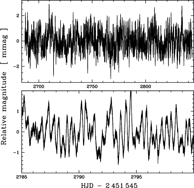
Figure 1:
The total CoRoT light curve ( top) and a zoom ( bottom) of HR 7349. This light curve is
detrended with a polynomial fit (order 8), which only affects frequencies below 6 |
| Open with DEXTER | |
![]() Hya was observed with the CoRoT satellite for
5 consecutive months. CoRoT was launched on 2006 December 27
from Baïkonur cosmodrome on a Soyuz Fregat II-1b launcher. The raw
photometric data acquired with
CoRoT were reduced by
the CoRoT team. A detailed description of how photometric data are
extracted for the seismology field was presented in Baglin (2006).
A summary can be found in Appourchaux et al. (2008).
Hya was observed with the CoRoT satellite for
5 consecutive months. CoRoT was launched on 2006 December 27
from Baïkonur cosmodrome on a Soyuz Fregat II-1b launcher. The raw
photometric data acquired with
CoRoT were reduced by
the CoRoT team. A detailed description of how photometric data are
extracted for the seismology field was presented in Baglin (2006).
A summary can be found in Appourchaux et al. (2008).
In the seismofield, CoRoT obtains one measurement every 32 s. The
observations lasted for 156.64 days from May 11th to October 15th
2007.
The light curve shows near-continuous coverage over the 5 months,
with only a small number of
gaps due mainly to the passage of CoRoT across the South Atlantic
Anomaly. These short gaps were filled by suitable interpolation (Baglin
2006),
without any influence on the mode extraction because it
only affects the amplitude of frequencies far above the oscillation range of our target (see Fig. 2).
The duty cycle for HR 7349 before interpolation was 90%. For the frequency analysis (see
Sect. 4), the light curve was detrended with a polynomial fit to remove the effect of the aging of the CCDs (see Auvergne et al. 2009).
This detrending has no consequence
on the amplitude or frequency of oscillation modes, since it only affects the power spectrum for frequencies lower than 6 ![]() Hz.
The light curve shows variations of a timescale of 8-9 h and peak-to-peak amplitudes of 1-3 mmag (see Fig. 1). This signal is a superposition of tens of smaller
modes with similar periods (see Sect. 4).
Hz.
The light curve shows variations of a timescale of 8-9 h and peak-to-peak amplitudes of 1-3 mmag (see Fig. 1). This signal is a superposition of tens of smaller
modes with similar periods (see Sect. 4).
| Figure 2:
Power spectra of the original data (grey) and interpolated data (black). The range of the oscillation is zoomed in the inset.
The interpolation drastically reduces the amplitude of aliases, in particular the one at 23 |
|
| Open with DEXTER | |
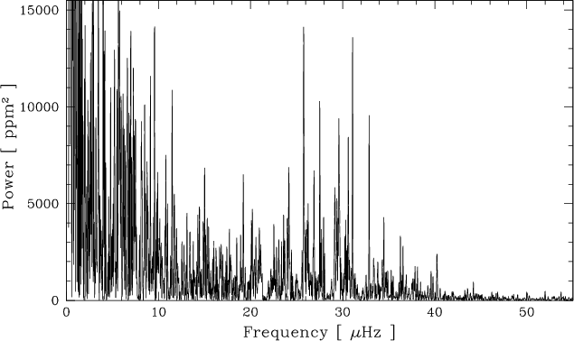
4 Frequency analysis
4.1 Noise determination
| Figure 3: Power density spectrum of the photometric time series of HR 7349 and a multi-component function (black line) fitted to the heavily smoothed power density spectrum. The function is the superposition of three power-law components (dashed lines), white noise (horizontal dashed line) and a power excess hump approximated by a Gaussian function. |
|
| Open with DEXTER | |
We computed the power spectra of CoRoT light curves with both gaps and interpolated points (see Sect. 3). The resulting
power spectra are quasi-identical, the interpolation not affecting the oscillations but suppressing the
aliases (the most important of which lies at 23 ![]() Hz).
We thus analyze the interpolated time series with negligible alias amplitudes.
The time base of the observations gives a formal resolution of 0.07
Hz).
We thus analyze the interpolated time series with negligible alias amplitudes.
The time base of the observations gives a formal resolution of 0.07 ![]() Hz.
The power (density) spectrum of the time series, shown in Figs. 3 and 4, exhibits a series of peaks between 20 and 40
Hz.
The power (density) spectrum of the time series, shown in Figs. 3 and 4, exhibits a series of peaks between 20 and 40 ![]() Hz, exactly where the solar-like oscillations
are expected for this star. The power density spectrum is independent of the observing window: this is
achieved by multiplying the power by the effective length of the
observing run (we have to divide by the resolution for equidistant data), which is calculated to be the
reciprocal of the area beneath the spectral window in power (Kjeldsen et al. 2005).
We note that to obtain the same normalisation as in Baudin et al. (2005), we multiply the power by the effective length of the observation divided by four.
Typically for such a power spectrum, the noise has two components:
Hz, exactly where the solar-like oscillations
are expected for this star. The power density spectrum is independent of the observing window: this is
achieved by multiplying the power by the effective length of the
observing run (we have to divide by the resolution for equidistant data), which is calculated to be the
reciprocal of the area beneath the spectral window in power (Kjeldsen et al. 2005).
We note that to obtain the same normalisation as in Baudin et al. (2005), we multiply the power by the effective length of the observation divided by four.
Typically for such a power spectrum, the noise has two components:
- at high frequencies it is flat, indicative of the Poisson statistics of photon noise;
- towards the lowest frequencies, the power scales inversely with frequency, as expected for instrumental instabilities and noise of stellar origin like granulation.
|
(1) |
where this number N depends on the frequency coverage,
To model the power density spectrum, we added a white noise Pn and a power excess hump produced by the
oscillations, which was approximated by a Gaussian function
|
(2) |
The number of components N is determined iteratively: we first made a single component fit, and additional components were then added until they no longer improved the fit. In our case, we limited the number of components to three. We note that for this star, part of the low frequency variation is caused by the aging of the CCD. The timescales for the different noise sources (Bi) are
4.2 Search for a comb-like pattern
|
Figure 4: Power spectrum of the CoRoT observations of HR 7349. Only a polynomial fit was removed from the original data. |
| Open with DEXTER | |
Here D0 (which equals
The first step is to measure the large spacing that should appear at least between radial modes.
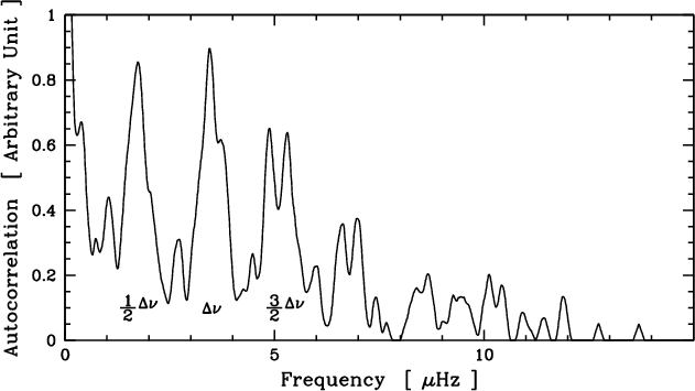
The power spectrum is autocorrelated to search for periodicity.
Each peak of this autocorrelation (see Fig. 5) corresponds to a structure present in the power spectrum.
One of the three strong groups of peaks at about 1.7, 3.5, and 5.2 ![]() Hz should correspond to the large spacing.
By visually inspecting the power spectrum, the value
of about 3.5
Hz should correspond to the large spacing.
By visually inspecting the power spectrum, the value
of about 3.5 ![]() Hz is adopted as the large separation, the two others are spacings between the
Hz is adopted as the large separation, the two others are spacings between the ![]() = 0 and
= 0 and ![]() = 1 modes. This large separation value is
in good agreement with the scaled value from the solar case (see Sect. 2.4).
= 1 modes. This large separation value is
in good agreement with the scaled value from the solar case (see Sect. 2.4).
|
Figure 5:
Autocorrelation of the slightly smoothed power spectrum. The large spacing, as well as separations between |
| Open with DEXTER | |
4.3 Extraction of mode parameters
The power spectra in Figs. 6 and 7 clearly exhibit a regularity that allows us to identify ![]() = 0 to
= 0 to ![]() = 2 modes.
Each mode consists of several peaks, which is the clear signature of a
finite lifetime shorter than the observing time span. In order to
determine the mode frequencies, as well as amplitude and lifetime of
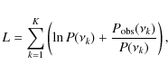
the modes, we fitted the power
spectrum using a maximum likelihood estimation (MLE) method.
MLE has been applied widely in the helioseismic community (e.g., see
Schou 1992; Appourchaux et al. 1998; and Chaplin et al. 2006).
Our program uses the IDL routines developed by Appourchaux (1998). This method has already been used with success for the red giant
= 2 modes.
Each mode consists of several peaks, which is the clear signature of a
finite lifetime shorter than the observing time span. In order to
determine the mode frequencies, as well as amplitude and lifetime of
the modes, we fitted the power
spectrum using a maximum likelihood estimation (MLE) method.
MLE has been applied widely in the helioseismic community (e.g., see
Schou 1992; Appourchaux et al. 1998; and Chaplin et al. 2006).
Our program uses the IDL routines developed by Appourchaux (1998). This method has already been used with success for the red giant ![]() Oph (Barban et al. 2007).
Oph (Barban et al. 2007).
The modelled power spectrum for a series of M oscillation modes, P(![]() ), is
), is
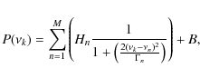
|
(4) |
where Hn is the height of the Lorentzian profile,
|
(5) |
where K is the number of bins, i.e., the number of Fourier frequencies.
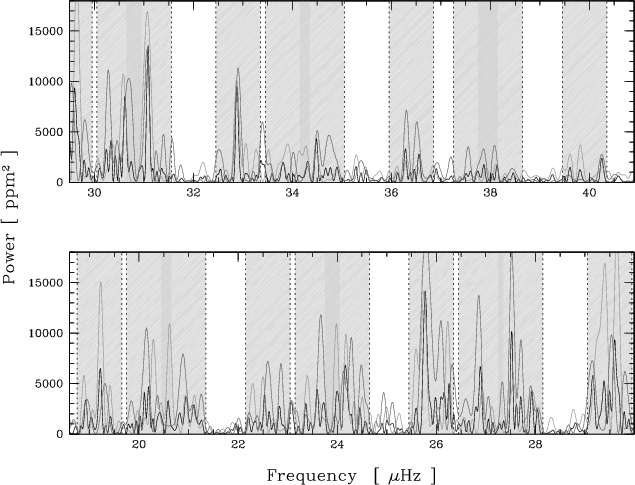
|
Figure 6:
Power spectra of the whole dataset (black) and of the two half-long
subsets (grey). The frequencies of the oscillation peaks change from
one subset to the other, which is a sign of a finite lifetime. The
initial guess for the identification of modes are indicated by shaded
regions: these regions are regularly spaced in agreement with the large
separation deduced from the autocorrelation. Every second region has a
structure more simple and narrow, corresponding to our identification
of |
| Open with DEXTER | |
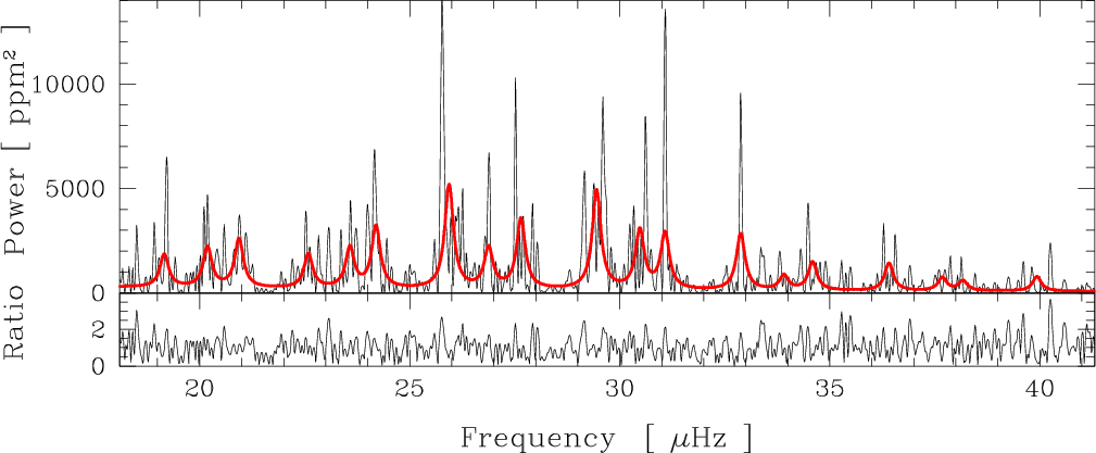
|
Figure 7: Top: Lorentzian fit (thick red line) of the observed power spectrum assuming the same lifetime for all the oscillation modes. Bottom: ratio of the observed spectrum over the Lorentzian fit (in amplitude). As expected, this ratio does not show any correlation with the fit. |
| Open with DEXTER | |
Only a few peaks belong to a given mode, indicating a lifetime longer than 10 days. It is thus also difficult to derive the correct Lorentzian shape for each mode. Therefore some parameters were fixed to avoid incorrect parameter determinations:
- the noise was determined independently of the MLE method (see Sect. 4.1);
- since no difference between the shapes of modes of different degree
 is detected and the value
of
is detected and the value
of  is extremely small, resulting in an
expected rotational splitting value smaller than 0.03
is extremely small, resulting in an
expected rotational splitting value smaller than 0.03  Hz, we assumed that it is zero;
- when fitting all modes without fixing the width of the
Lorentzian envelope, we clearly saw that the fit was not robust enough
to provide an accurate determination of all mode parameters.
The method was thus first to find a mean value for the Lorentzian width
and to fix this mean value for all modes.
The mean width of the Lorentzian is obtained by individually fitting
all modes and by taking their mean,
rejecting the values that obviously correspond to a poor fit.
The determined mean
is 0.25
 0.06 Hz, which
corresponds to a mode lifetime of 14.7
+4.7-2.9 d.
The use of sub-series show the stochastic nature of the mode excitation
caused by the different fine structure of peaks in each spectrum, and
give an indication of their width.
We note that we also checked that no significant width difference was
found for modes with different
degrees
(by comparing their mode-width means).
0.06 Hz, which
corresponds to a mode lifetime of 14.7
+4.7-2.9 d.
The use of sub-series show the stochastic nature of the mode excitation
caused by the different fine structure of peaks in each spectrum, and
give an indication of their width.
We note that we also checked that no significant width difference was
found for modes with different
degrees
(by comparing their mode-width means).
The large and small separations are shown in Fig. 9. The mean large separation has a value of ![]() = 3.47
= 3.47 ![]() 0.12
0.12 ![]() Hz, and the values for different
degrees
Hz, and the values for different
degrees ![]() ,
,
![]() ,
are:
,
are:
![]() = 3.45
= 3.45 ![]() 0.12
0.12 ![]() Hz,
Hz,
![]() = 3.46
= 3.46 ![]() 0.07
0.07 ![]() Hz, and
Hz, and
![]() = 3.50
= 3.50 ![]() 0.19
0.19 ![]() Hz.
We can identify a small oscillation of the large spacing that varies with frequency, which is a clear signature of the
second helium ionization zone (see e.g., Monteiro & Thompson 1998).
The small separation has a mean value
of
Hz.
We can identify a small oscillation of the large spacing that varies with frequency, which is a clear signature of the
second helium ionization zone (see e.g., Monteiro & Thompson 1998).
The small separation has a mean value
of
![]() = 0.65
= 0.65 ![]() 0.10
0.10 ![]() Hz and seems to decrease with frequency.
The small value of the frequency difference between these modes make their frequency determination more uncertain than that of
Hz and seems to decrease with frequency.
The small value of the frequency difference between these modes make their frequency determination more uncertain than that of
![]() = 1 modes, which are not affected by neighbouring modes.
= 1 modes, which are not affected by neighbouring modes.
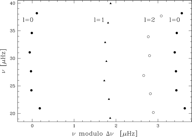
|
Figure 8:
Echelle diagram of identified modes with a large separation of
|
| Open with DEXTER | |
Table 1: Frequency and amplitude of identified modes.
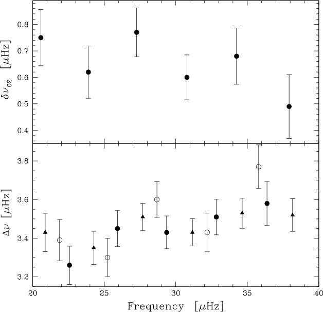
|
Figure 9: Top: small spacing versus frequency. Bottom: large spacing versus frequency. The variations of the large separation with frequency show a clear oscillation. The symbols used are the same as for Fig. 8. |
| Open with DEXTER | |
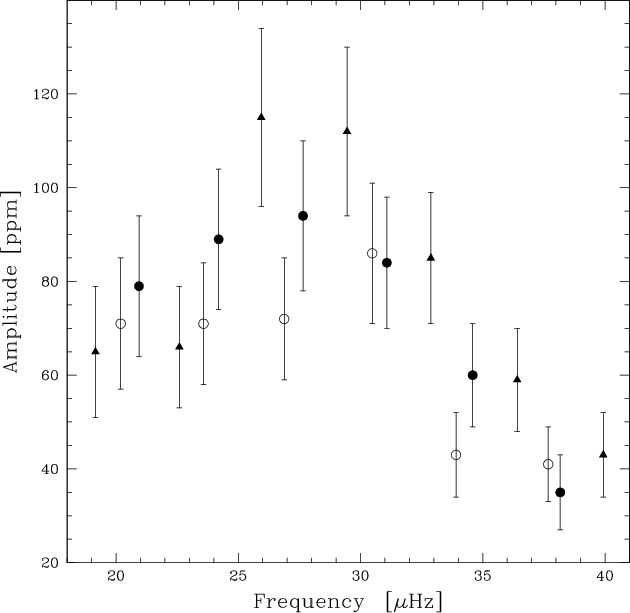
4.4 Oscillation amplitudes
The fit of the Lorentzian profiles to the power spectrum infers the height of all oscillation modes.
Since the modes are resolved and because of the normalization of the power spectrum, the RMS
amplitude is measured to be (see Baudin et al. 2005)

|
(6) |
where H and
As noticed by Kjeldsen et al. (2005), measurements made on different stars with different instruments using different techniques, in different
spectral lines or bandpasses, have different sensitivity to the oscillations. It is thus important to
derive a bolometric amplitude that is independent of the
instrument used. We computed the maximum bolometric amplitude of the ![]() = 0 modes, because their
visibility coefficients do not depend on the inclination of the star.
According to Michel et al. (2009), who derived the CoRoT response for radial modes, radial-mode
amplitudes of HR 7349 must be divided by 1.16 to obtain
the bolometric amplitudes. We find that
= 0 modes, because their
visibility coefficients do not depend on the inclination of the star.
According to Michel et al. (2009), who derived the CoRoT response for radial modes, radial-mode
amplitudes of HR 7349 must be divided by 1.16 to obtain
the bolometric amplitudes. We find that
![]() = 81 ppm, which corresponds to 32 times the solar value (Michel et al. 2009).
The scaling laws for both the large separation and the frequency of the maximum amplitude (Kjeldsen & Bedding 1995), coupled with the non-asteroseismic constraints,
infer
a mass for HR 7349 of about 1.2
= 81 ppm, which corresponds to 32 times the solar value (Michel et al. 2009).
The scaling laws for both the large separation and the frequency of the maximum amplitude (Kjeldsen & Bedding 1995), coupled with the non-asteroseismic constraints,
infer
a mass for HR 7349 of about 1.2 ![]() The derived amplitude is in good agreement with a scaling function
The derived amplitude is in good agreement with a scaling function
![]() ,
with s close to 0.8,
which is in-between the values given by Samadi et al. (2007; s=0.7) and Kjeldsen & Bedding (1995; s=1).
,
with s close to 0.8,
which is in-between the values given by Samadi et al. (2007; s=0.7) and Kjeldsen & Bedding (1995; s=1).
|
Figure 10: Amplitude of the oscillation modes versus frequency. The symbols used are the same as for Fig. 8. |
| Open with DEXTER | |
5 Conclusion
The red giant star HR 7349 has been observed for about 156 days by the CoRoT satellite. These observations have yielded a clear detection of p-mode oscillations. As already mentioned by De Ridder et al. (2009), non-radial modes are observed in red giants. Nineteen identifiable modes of degreeAll modes of the same degree are aligned in the echelle diagram, which is a sign of modes that follow the asymptotic relation.
However, the separation between ![]() =1 and
=1 and ![]() =0 modes is not fully compatible with
this asymptotic relation. All frequency patterns
are theoretically expected for red giants (Dupret et al. 2009), from very complex to regular:
our observations correspond to a red giant for which the radiative
damping of non-radial modes is large and only radial and non-radial modes completely trapped in the envelope can be observed.
=0 modes is not fully compatible with
this asymptotic relation. All frequency patterns
are theoretically expected for red giants (Dupret et al. 2009), from very complex to regular:
our observations correspond to a red giant for which the radiative
damping of non-radial modes is large and only radial and non-radial modes completely trapped in the envelope can be observed.
By fitting Lorentzian profiles to the power spectrum, it has also been
possible to unambiguously derive, for the first time for a red giant, a
mean line-width of 0.25 ![]() Hz corresponding to a mode lifetime of 14.7 days. This lifetime
is in agreement with the scaling law
Hz corresponding to a mode lifetime of 14.7 days. This lifetime
is in agreement with the scaling law
![]() suggested by Chaplin et al. (2009),
although is a little too long. This relation however has yet to be
verified for a larger number of red giants with different physical
properties.
The theoretical study of this red giant, including asteroseismic and
non-asteroseismic constraints, will be the subject of a second paper.
suggested by Chaplin et al. (2009),
although is a little too long. This relation however has yet to be
verified for a larger number of red giants with different physical
properties.
The theoretical study of this red giant, including asteroseismic and
non-asteroseismic constraints, will be the subject of a second paper.
F.C. is a postdoctoral fellow of the Fund for Scientific Research, Flanders (FWO). AM is a postdoctoral researcher of the ``Fonds de la recherche scientifique'' FNRS, Belgium. T.K. is supported by the Canadian Space Agency and the Austrian Science Found (FWF). The research leading to these results has received funding from the Research Council of K.U. Leuven under grant agreement GOA/2008/04, from the Belgian PRODEX Office under contract C90309: CoRoT Data Exploitation, and from the FWO-Vlaanderen under grant O6260. We thank T. Appourchaux for helpful comments.
References
- Aigrain, S., Favata, F., & Gilmore, G. 2004, A&A, 414, 1139 [Google Scholar]
- Alonso, A., Arribas, S., & Martinez-Roger, C. 1999, A&AS, 140, 261 [Google Scholar]
- Andersen, B., Appourchaux, T., & Crommelnynck, D. 1998, in Sounding solar and stellar interiors, ed. Provost, & Schmider, 181, 147 [Google Scholar]
- Appourchaux, T., Gizon, L., & Rabello-Soares, M. C. 1998, A&AS, 132, 107 [Google Scholar]
- Appourchaux, T., Michel, E., Auvergne, M., et al. 2008, A&A, 488, 705 [Google Scholar]
- Arenou, F., Grenon, M., & Gomez, A. 1992, A&A, 258, 104 [Google Scholar]
- Auvergne, M., Bodin, P., Boisnard, L., et al. 2009, A&A, 506, 411 [Google Scholar]
- Baglin, A. 2006, ESA SP-1306, The CoRoT mission, ed. M. Fridlund, A. Baglin, J. Lochard and L. Conroy (Noordwijk, The Nederlands) [Google Scholar]
- Barban, C., De Ridder, J., Mazumdar, A., et al. 2004, ESA SP-559, SOHO 14 Helio- and Asteroseismology, ed. D. Danesy, 113 [Google Scholar]
- Barban, C., Matthews, J. M., De Ridder, J., et al. 2007, A&A, 468, 1033 [Google Scholar]
- Baudin, F., Samadi, R., Goupil, M.-J., et al. 2005, A&A, 433, 349 [Google Scholar]
- Bedding, T. R., & Kjeldsen H. 2007, CoAst, 150, 106 [Google Scholar]
- Burki, G., et al. 2008, http://obswww.unige.ch/gcpd/ph13.html [Google Scholar]
- Carrier, F., Eggenberger, P., & Leyder, J. C. 2008, JPHCS, 118, 2047 [NASA ADS] [Google Scholar]
- Chaplin, W. J., Appourchaux, T., Baudin, F., et al. 2006, MNRAS, 369, 985 [NASA ADS] [CrossRef] [Google Scholar]
- Chaplin, W. J., Houdek, G., Karoff, C., et al. 2009, A&A, 500, L21 [Google Scholar]
- Christensen-Dalsgaard, J. 2004, Sol. Phys., 220, 137 [NASA ADS] [CrossRef] [Google Scholar]
- Christensen-Dalsgaard, J., Bedding, T. R., & Kjeldsen, H. 1995, ApJ, 443, L29 [NASA ADS] [CrossRef] [Google Scholar]
- Dupret, M.-A., Belkacem, K., Samadi, R., et al. 2009, A&A, 506, 57 [Google Scholar]
- De Ridder, J., Barban, C., Carrier, F., et al. 2006, A&A, 448, 689 [Google Scholar]
- De Ridder, J., Barban, C., Baudin., F., et al. 2009, Nature, 459, 398 [Google Scholar]
- Fernandes, J., & Monteiro, M. J. P. F. G. 2003, A&A, 399, 243 [Google Scholar]
- Flower, P. 1996, ApJ, 469, 355 [NASA ADS] [CrossRef] [Google Scholar]
- Frandsen, S., Carrier, F., Aerts, C., et al. 2002, A&A, 394, L5 [Google Scholar]
- Kjeldsen, H., & Bedding, T. 1995, A&A, 293, 87 [Google Scholar]
- Kjeldsen, H., Bedding, T., Butler, R. P., et al. 2005, ApJ, 635, 1281 [NASA ADS] [CrossRef] [Google Scholar]
- Harvey, J. 1985, in Future Missions in Solar, Heliospheric, & Space Plasma Physics, ed. Rolfe & Battrick, ESA SP, 235, 199 [Google Scholar]
- Hekker, S., & Meléndez, J. 2007, A&A, 475, 1003 [Google Scholar]
- Hekker, S., Kallinger, T., Baudin, F., et al. 2009, A&A, 506, 465 [Google Scholar]
- Lejeune, T., Cuisinier, F., & Buser, R. 1998, A&AS, 130, 65 [Google Scholar]
- Libbrecht, K. G. 1992, ApJ, 387, 712 [NASA ADS] [CrossRef] [Google Scholar]
- Michel, E., Samadi, R., Baudain, F., et al. 2009, A&A 495, 979 [Google Scholar]
- Monteiro, M. J. P. F. G., & Thompson, M. J. 1998, IAU Symp., 185, 317 [Google Scholar]
- Samadi, R., Georgobiani, D., Trampedach, R., et al. 2007, A&A, 463, 297 [Google Scholar]
- Santos, N. C., Mayor, M., Naef, D., et al. 2002, A&A, 392, 215 [Google Scholar]
- Schou, J. 1992, Ph.D. Thesis (Denmark: Aarhus Universitet) [Google Scholar]
- Stello, D., Kjeldsen, H., Bedding, T. R., & Buzasi, D. 2006, A&A, 448, 709 [Google Scholar]
- Tarrant, N. J., Chaplin, W. J., Elsworth, Y. P., et al. 2008, CoAst, 157, 92 [NASA ADS] [Google Scholar]
- Tassoul, M. 1980, ApJS, 43, 469 [NASA ADS] [CrossRef] [Google Scholar]
- Toutain, T., & Appourchaux, T. 1994, A&A, 289, 649 [Google Scholar]
- van Leeuwen, F. 2007, A&A, 474, 653 [Google Scholar]
Footnotes
- ... CoRoT
- The CoRoT space mission has been developed and is operated by CNES, with the contribution of Austria, Belgium, Brazil, ESA, Germany and Spain.
All Tables
Table 1: Frequency and amplitude of identified modes.
All Figures
|
|
Figure 1:
The total CoRoT light curve ( top) and a zoom ( bottom) of HR 7349. This light curve is
detrended with a polynomial fit (order 8), which only affects frequencies below 6 |
| Open with DEXTER | |
| In the text | |
| |
Figure 2:
Power spectra of the original data (grey) and interpolated data (black). The range of the oscillation is zoomed in the inset.
The interpolation drastically reduces the amplitude of aliases, in particular the one at 23 |
| Open with DEXTER | |
| In the text | |
| |
Figure 3: Power density spectrum of the photometric time series of HR 7349 and a multi-component function (black line) fitted to the heavily smoothed power density spectrum. The function is the superposition of three power-law components (dashed lines), white noise (horizontal dashed line) and a power excess hump approximated by a Gaussian function. |
| Open with DEXTER | |
| In the text | |
|
|
Figure 4: Power spectrum of the CoRoT observations of HR 7349. Only a polynomial fit was removed from the original data. |
| Open with DEXTER | |
| In the text | |
|
|
Figure 5:
Autocorrelation of the slightly smoothed power spectrum. The large spacing, as well as separations between |
| Open with DEXTER | |
| In the text | |
|
|
Figure 6:
Power spectra of the whole dataset (black) and of the two half-long
subsets (grey). The frequencies of the oscillation peaks change from
one subset to the other, which is a sign of a finite lifetime. The
initial guess for the identification of modes are indicated by shaded
regions: these regions are regularly spaced in agreement with the large
separation deduced from the autocorrelation. Every second region has a
structure more simple and narrow, corresponding to our identification
of |
| Open with DEXTER | |
| In the text | |
|
|
Figure 7: Top: Lorentzian fit (thick red line) of the observed power spectrum assuming the same lifetime for all the oscillation modes. Bottom: ratio of the observed spectrum over the Lorentzian fit (in amplitude). As expected, this ratio does not show any correlation with the fit. |
| Open with DEXTER | |
| In the text | |
|
|
Figure 8:
Echelle diagram of identified modes with a large separation of
|
| Open with DEXTER | |
| In the text | |
|
|
Figure 9: Top: small spacing versus frequency. Bottom: large spacing versus frequency. The variations of the large separation with frequency show a clear oscillation. The symbols used are the same as for Fig. 8. |
| Open with DEXTER | |
| In the text | |
|
|
Figure 10: Amplitude of the oscillation modes versus frequency. The symbols used are the same as for Fig. 8. |
| Open with DEXTER | |
| In the text | |
Copyright ESO 2010
Current usage metrics show cumulative count of Article Views (full-text article views including HTML views, PDF and ePub downloads, according to the available data) and Abstracts Views on Vision4Press platform.
Data correspond to usage on the plateform after 2015. The current usage metrics is available 48-96 hours after online publication and is updated daily on week days.
Initial download of the metrics may take a while.