| Issue |
A&A
Volume 509, January 2010
|
|
|---|---|---|
| Article Number | A63 | |
| Number of page(s) | 11 | |
| Section | Galactic structure, stellar clusters, and populations | |
| DOI | https://doi.org/10.1051/0004-6361/200912641 | |
| Published online | 19 January 2010 | |
Stellar interactions in dense and sparse star clusters
C. Olczak1 - S. Pfalzner1 - A. Eckart1,2
1 - I. Physikalisches Institut, Universität zu Köln, Zülpicher Str.77, 50937 Köln, Germany
2 - Max-Planck-Institut für Radioastronomie, Auf dem Hügel 69, 53121 Bonn, Germany
Received 5 June 2009 / Accepted 2 November 2009
Abstract
Context. Stellar encounters potentially affect the evolution
of the protoplanetary discs in the Orion Nebula Cluster (ONC). However,
the role of encounters in other cluster environments is less known.
Aims. We investigate the effect of the encounter-induced disc-mass loss in different cluster environments.
Methods. Starting from an ONC-like cluster we vary the cluster
size and density to determine the correlation of the collision time
scale and disc-mass loss. We use the NBODY6 ++ code to model the dynamics of these clusters and analyse the disc-mass loss due to encounters.
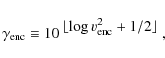
Results. We find that the encounter rate strongly depends on the
cluster density but remains rather unaffected by the size of the
stellar population. This dependency translates directly into the effect
on the encounter-induced disc-mass loss. The essential outcome of the
simulations are: i) even in clusters of four times lower density than
the ONC, the effect of encounters is still apparent; ii) the density of
the ONC itself marks a threshold: in less dense and less massive
clusters it is the massive stars that dominate the encounter-induced
disc-mass loss, whereas in denser and more massive clusters the
low-mass stars play the major role for the disc-mass removal.
Conclusions. It seems that in the central regions of young dense
star clusters - the common sites of star formation - stellar encounters
do affect the evolution of the protoplanetary discs. With higher
cluster density low-mass stars become more heavily involved in this
process. These results can also be applied to extreme stellar systems:
in the case of the Arches cluster one would expect stellar encounters
to destroy the discs of most of the low- and high-mass stars in several
hundred thousand years, whereas intermediate mass stars are able to
retain their discs to some extent even under these harsh environmental
conditions.
Key words: stellar dynamics - methods: numerical - stars: pre-main sequence - circumstellar matter
1 Introduction
According to current knowledge, planetary systems form from the
accretion discs around young stars. These young stars are in most cases
not isolated,
but are part of a cluster (e.g. Lada & Lada 2003). Densities in these cluster environments vary considerably, spanning a range of
10 pc-3 (e.g. ![]() Chameleontis) to 106 pc-3 (e.g. Arches Cluster). Though it is known that discs disperse over time
(Currie et al. 2008; Hillenbrand 2002; Haisch et al. 2001; Sicilia-Aguilar et al. 2006) and that in dense clusters (
Chameleontis) to 106 pc-3 (e.g. Arches Cluster). Though it is known that discs disperse over time
(Currie et al. 2008; Hillenbrand 2002; Haisch et al. 2001; Sicilia-Aguilar et al. 2006) and that in dense clusters (
![]() pc-3)
the disc frequency seems to be lower in the core (e.g. Balog et al. 2007),
it is an open question as to how far interactions with the surrounding
stars influence the planet formation in clusters of different
densities.
pc-3)
the disc frequency seems to be lower in the core (e.g. Balog et al. 2007),
it is an open question as to how far interactions with the surrounding
stars influence the planet formation in clusters of different
densities.
Two major mechanisms are potentially able to strongly affect the evolution of protoplanetary discs and planets in a cluster environment: photoevaporation and gravitational interactions. Photoevaporation causes the heating and evaporation of disc matter by the intense UV radiation from massive stars. First models of photoevaporation were developed by Johnstone et al. (1998) and Störzer & Hollenbach (1999) (see also references in Hollenbach et al. 2000) and have been much improved in the past years (Drake et al. 2009; Alexander et al. 2006; Gorti & Hollenbach 2009; Clarke et al. 2001; Alexander et al. 2005; Ercolano et al. 2008; Matsuyama et al. 2003; Johnstone et al. 2004). Gravitational interactions are another important effect on the population of stars, discs and planets in a cluster environment. An encounter between a circumstellar disc and a nearby passing star can lead to a significant loss of mass and angular momentum from the disc. While such isolated encounters have been studied in a large variety (Clarke & Pringle 1993; Ostriker 1994; Heller 1995; Pfalzner et al. 2005; Kley et al. 2008; Moeckel & Bally 2006; Hall 1997; Heller 1993; Hall et al. 1996; Pfalzner 2004; Moeckel & Bally 2007b), only a few numerical studies have directly investigated the effect of stellar encounters on circumstellar discs in a dense cluster environment (Adams et al. 2006; Scally & Clarke 2001).
It has been shown only recently by numerical simulations that stellar encounters do have an effect on the discs surrounding stars in a young dense cluster Moeckel & Bally 2006; Pfalzner & Olczak 2007b; Olczak et al. 2006; Pfalzner 2006; Pfalzner & Olczak 2007a; Moeckel & Bally 2007b; Pfalzner et al. 2006; Moeckel & Bally 2007a; see also the review by Zinnecker & Yorke 2007. The massive stars in the centre of such a stellar cluster act as gravitational foci for the lower mass stars (Pfalzner et al. 2006). Discs are most affected when the masses of the stars involved in an encounter are unequal (Olczak et al. 2006; Moeckel & Bally 2007b), so it is the massive stars which dominate the encounter-induced disc-mass loss in the young dense clusters (Olczak et al. 2006). Observational evidence for this effect has been found by Olczak et al. (2008).
The numerical results obtained in our previous investigations are based on a dynamical model of the Orion Nebula Cluster (ONC) - one of the observationally most intensively studied young star cluster. It was demonstrated that in the ONC stellar encounters can have a significant impact on the evolution of the young stars and their surrounding discs (Olczak et al. 2006; Pfalzner & Olczak 2007a; Pfalzner 2006; Pfalzner et al. 2008,2006; Olczak et al. 2008). However, investigating one model star cluster is not sufficient to draw general conclusions - in fact, one could not answer questions as: How would things change in a denser cluster? Would a higher density inevitably imply that stellar encounters play a more important role in the star - and planet formation process? And what would the situation be like in more massive clusters? Would the larger number of stars - in particular massive stars - play a role?
Conclusive answers to these questions demand further numerical investigations covering a larger parameter space in cluster parameters. Here we realise this by modelling clusters as scaled versions of the standard ONC model with varying stellar numbers and sizes. The focus of this investigation is on the encounter-induced disc-mass loss. Throughout this work we assume that initially all stars are surrounded by protoplanetary discs. This is justified by observations that reveal disc fractions of nearly 100% in very young star clusters (e.g. Haisch et al. 2000; Hillenbrand 2005; Lada et al. 2000; Haisch et al. 2001). In Sect. 2 we outline briefly the observationally determined basic properties of the ONC, which serves as a reference model for the other cluster models. The computational method is described in Sect. 3 and the construction of the numerical models is outlined in Sect. 4. Afterwards we present results from a numerical approach to this problem in Sect. 5 and compare with analytical estimates in Sect. 6. The conclusion and discussion mark the last section of this paper.
2 Structure and dynamics of the ONC
The ONC is a rich stellar cluster with about 4000 members with masses of
![]() and a radial extension of
and a radial extension of
![]() 2.5 pc (Hillenbrand & Carpenter 2000; Hillenbrand & Hartmann 1998). Most of the objects are T Tauri stars. The mean stellar mass is about
2.5 pc (Hillenbrand & Carpenter 2000; Hillenbrand & Hartmann 1998). Most of the objects are T Tauri stars. The mean stellar mass is about
![]() and the half-mass radius
and the half-mass radius
![]() pc (Hillenbrand & Hartmann 1998). Recent studies
of the stellar mass distribution (Slesnick et al. 2004; Luhman et al. 2000; Hillenbrand & Carpenter 2000; Muench et al. 2002) reveal no significant
deviation from the generalised IMF of Kroupa (2002),
pc (Hillenbrand & Hartmann 1998). Recent studies
of the stellar mass distribution (Slesnick et al. 2004; Luhman et al. 2000; Hillenbrand & Carpenter 2000; Muench et al. 2002) reveal no significant
deviation from the generalised IMF of Kroupa (2002),
The mean age of the whole cluster has been estimated to be
The density and velocity distribution of the ONC resembles an isothermal sphere. The central number density
![]() in the inner 0.053 pc
reaches
in the inner 0.053 pc
reaches
![]() pc-3 (McCaughrean et al. 2002) and makes the ONC the densest nearby (<1 kpc) young stellar cluster. The
dense inner part of the ONC, also known as the Trapezium Cluster (TC), is characterised by
pc-3 (McCaughrean et al. 2002) and makes the ONC the densest nearby (<1 kpc) young stellar cluster. The
dense inner part of the ONC, also known as the Trapezium Cluster (TC), is characterised by
![]() pc and
pc and
![]() ,
or
,
or
![]() pc-3.
pc-3.
In the most detailed study on circumstellar discs in the Trapezium Cluster, Lada et al. (2000) found a fraction of 80-85% discs among the stellar population from the L-band excess. This agrees with an earlier investigation of the complete ONC in which Hillenbrand et al. (1998) report
a disc fraction of 50-90% (though relying only on
![]() colors) and justifies the assumption of a 100% primordial disc fraction in
the simulations presented here.
colors) and justifies the assumption of a 100% primordial disc fraction in
the simulations presented here.
We now describe the construction of the numerical cluster models that have been used in our simulations.
3 Computational method
The basic dynamical model of the ONC used here is described in Olczak et al. (2006), but we include several extensions discussed in
Pfalzner & Olczak (2007b). We summarise the main aspects of our model: the initial stellar population consists of 4000 members with masses of
between
![]() and
and
![]() sampled from the standard Kroupa IMF (see Eq. (1)). The system is initially in virial
equilibrium,
sampled from the standard Kroupa IMF (see Eq. (1)). The system is initially in virial
equilibrium,
where
For the generation of star cluster models in the present
investigation the initial radial density profile has been slightly
modified. In a first-order
approximation, the isothermal sphere,
![]() ,
represents the projected density distribution of the ONC, yet a flattening in the
core,
,
represents the projected density distribution of the ONC, yet a flattening in the
core,
![]() ,
,
![]() ,
,
![]() pc, is observed (Scally et al. 2005). Validating the initial setup by means of the best reproduction of the current projected
density distribution of the ONC after a simulation time of 1 Myr,
the evaluation of numerous initial configurations led to the following
best estimate of the initial three-dimensional density distribution:
pc, is observed (Scally et al. 2005). Validating the initial setup by means of the best reproduction of the current projected
density distribution of the ONC after a simulation time of 1 Myr,
the evaluation of numerous initial configurations led to the following
best estimate of the initial three-dimensional density distribution:
![$\displaystyle \rho_0(r) =
\left\{ \begin{array}{ll}
\rho_0~(r/R_{{\rm core}})^{...
...ore}},R] \\
\qquad 0 & , \quad r \in (R,\infty] \\
\end{array}\right. \quad ,$](/articles/aa/full_html/2010/01/aa12641-09/img42.png)
where
Moreover, the generation of the high-mass end of the mass function has
been modified. In the case of the ONC the upper mass was chosen to be
50
![]() ,
because this value corresponds to the mass of the most massive stellar
system in the ONC. However, stars with larger masses are expected
to form in more massive clusters (Oey & Clarke 2005; Weidner & Kroupa 2006). Thus in the framework of this numerical investigation the upper mass
limit has been set to the currently accepted fundamental upper mass limit,
,
because this value corresponds to the mass of the most massive stellar
system in the ONC. However, stars with larger masses are expected
to form in more massive clusters (Oey & Clarke 2005; Weidner & Kroupa 2006). Thus in the framework of this numerical investigation the upper mass
limit has been set to the currently accepted fundamental upper mass limit,
![]() (Koen 2006; Oey & Clarke 2005; Maíz Apellániz et al. 2007; Zinnecker & Yorke 2007; Weidner & Kroupa 2006; Figer 2005).
(Koen 2006; Oey & Clarke 2005; Maíz Apellániz et al. 2007; Zinnecker & Yorke 2007; Weidner & Kroupa 2006; Figer 2005).
The choice of a fixed upper mass limit, though in disagreement with the well-established non-trivial correlation of the mass of a star cluster and its most massive member (e.g. Maschberger & Clarke 2008; Weidner & Kroupa 2006; Larson 2003), was motivated by the fact that the exact relation is not known. However, a comparison with the ``sorted sampling algorithm'' of Weidner & Kroupa (2006) in Table 1 shows that - at least in a statistical sense - the exact prescription for the generation of the maximum stellar mass in a cluster is not as important as it might seem. The values obtained by random sampling are only slightly larger than those from sorted sampling.
Table 1: Averaged initial parameters of the two families of cluster models.
Stellar encounters in dense clusters can lead to a significant transport of mass and angular momentum in protoplanetary discs
(Olczak et al. 2006; Pfalzner & Olczak 2007a; Pfalzner et al. 2006). In the present investigation we assume that all discs are of a low mass, i.e. a
low mass ratio of disc and central star,
![]() ,
which agrees with observations of the ONC
(Bally et al. 1998; Williams et al. 2005; Mann & Williams 2009). We use Eq. (1) from Pfalzner et al. (2006) to keep track of the
relative disc-mass loss of each star-disc system due to
encounters. Approaches of stars are only considered to be encounters if
the calculated
relative disc-mass loss is higher than 3%, corresponding to the 1
,
which agrees with observations of the ONC
(Bally et al. 1998; Williams et al. 2005; Mann & Williams 2009). We use Eq. (1) from Pfalzner et al. (2006) to keep track of the
relative disc-mass loss of each star-disc system due to
encounters. Approaches of stars are only considered to be encounters if
the calculated
relative disc-mass loss is higher than 3%, corresponding to the 1![]() error in our simulations of star-disc encounters. In this case the
relative disc-mass loss is independent of the disc-mass and depends
only on the mass ratio of the interacting stars and the orbital
parameters
(see Pfalzner et al. 2006).
Our estimate of the accumulated disc-mass loss is an upper limit
because the underlying formula is only valid for co-planar, prograde
encounters, which are the most perturbing. A simplified prescription
assigns stars into one of two distinct groups: if the
relative disc-mass loss exceeds 90% of the initial disc mass,
stars are marked as ``discless''; otherwise they are termed ``star-disc
systems''. As
in our previous investigations, the determination of the disc-mass loss
involves two different models of the initial distribution of disc
sizes:
i) scaled disc sizes
error in our simulations of star-disc encounters. In this case the
relative disc-mass loss is independent of the disc-mass and depends
only on the mass ratio of the interacting stars and the orbital
parameters
(see Pfalzner et al. 2006).
Our estimate of the accumulated disc-mass loss is an upper limit
because the underlying formula is only valid for co-planar, prograde
encounters, which are the most perturbing. A simplified prescription
assigns stars into one of two distinct groups: if the
relative disc-mass loss exceeds 90% of the initial disc mass,
stars are marked as ``discless''; otherwise they are termed ``star-disc
systems''. As
in our previous investigations, the determination of the disc-mass loss
involves two different models of the initial distribution of disc
sizes:
i) scaled disc sizes
![]() with
with
![]() ,
which is equivalent to the assumption of a fixed
force at the disc boundary; and ii) equal disc sizes with
,
which is equivalent to the assumption of a fixed
force at the disc boundary; and ii) equal disc sizes with
![]() .
Whenever results are presented, we will specify which
of these two distributions has been used.
.
Whenever results are presented, we will specify which
of these two distributions has been used.
4 Numerical models
For the present study we have set up a variety of scaled versions of
the standard ONC model cluster with varying sizes and stellar numbers.
In total,
eleven cluster models have been set up (see Table 1).
They form two parametric groups, the ``density-scaled'' (D0-D5) and
the ``size-scaled'' (S0-S5) group, both containing six clusters with
stellar numbers of 1000, 2000, 4000, 8000, 16 000, and
32 000, respectively. Models
D2 and S2 are identical and correspond to the standard ONC model with
the adopted higher stellar upper mass limit,
![]() .
The other ten cluster models have been set up as scaled representations
of ONC-like clusters. As in the case of the numerical model of the ONC,
for each cluster model a set of simulations has been performed with
varying random configurations of positions, velocities, and masses,
according to the given distributions, to minimise the effect of
statistical uncertainties. For the clusters with 1000, 2000, 4000,
8000, 16 000, and
32 000 particles, a number of 200, 100, 100, 50, 20, and
20 simulations seemed appropriate to provide sufficiently robust
results.
.
The other ten cluster models have been set up as scaled representations
of ONC-like clusters. As in the case of the numerical model of the ONC,
for each cluster model a set of simulations has been performed with
varying random configurations of positions, velocities, and masses,
according to the given distributions, to minimise the effect of
statistical uncertainties. For the clusters with 1000, 2000, 4000,
8000, 16 000, and
32 000 particles, a number of 200, 100, 100, 50, 20, and
20 simulations seemed appropriate to provide sufficiently robust
results.
It has to be noted that these ``artificial'' stellar systems are not just theoretical models but have counterparts as well in the observational catalogues of star clusters: the young star cluster NGC 2024 (e.g. Haisch et al. 2000; Liu et al. 2003; Bik et al. 2003) is well represented by the 1000 particle model, whereas the 16000 particle model has its counterpart in the massive cluster NGC 3603 (e.g. Stolte et al. 2006; de Pree et al. 1999; Stolte et al. 2004).
Density-scaled cluster models
The six density-scaled cluster models (D0-D5) have been simulated with the same initial size as the ONC (R=2.5 pc). Due to the adopted number
density distribution, which is roughly represented by
![]() ,
the density of the models scales as the stellar number,
,
the density of the models scales as the stellar number,
though for an exact treatment one would have to consider the steeper density profile of the core,
However, since the core population is not dominant in terms of the number, the clusters are characterised in good approximation by densities that are 1/4, 1/2, 1, 2, 4, and 8 times the density of the ONC (at any radius), respectively. These models are used to study the importance of the density for the effect of star-disc encounters in a cluster environment.
Size-scaled cluster models
Five more cluster models have been simulated with the same initial density as the ONC, but with varying extension. The set of size-scaled cluster models (S0-S5) is used to study the pure effect of the size of the stellar population. Due to the relation (4), the initial size of these clusters scales as the stellar number and was set up with 1/4, 1/2, 1, 2, 4 and 8 times the initial size of the ONC, respectively.
![\begin{figure}
\par\includegraphics[angle=-90,width=8cm,clip]{12641f01.eps}
\end{figure}](/articles/aa/full_html/2010/01/aa12641-09/img65.png)
|
Figure 1: Projected density profiles of the density-scaled models compared to observational data. The initial profile (grey lines) and the profile at a simulation time of 1 Myr (black lines) are shown. From bottom to top the cluster models D0-D5 are marked in each colour regime by a short-dashed, long-dashed, solid, dotted, dot-long-dashed, and dot-short-dashed line, respectively. The observational data are from a compilation of McCaughrean et al. (2002) and Hillenbrand (1997). |
| Open with DEXTER | |
The initial parameters of the cluster models, for each model averaged over all configurations, are presented in
Table 1. Here the number density in the Trapezium Cluster,
![]() ,
is taken as a reference value for all
simulations. As expected, the density scales with the number of stars
for the density-scaled models, while it is rather constant for the
size-scaled
models. The velocity dispersion, which satisfies the relation
,
is taken as a reference value for all
simulations. As expected, the density scales with the number of stars
for the density-scaled models, while it is rather constant for the
size-scaled
models. The velocity dispersion, which satisfies the relation
shows the expected scaling of
5 Results of numerical simulations
In this section the results of the numerical simulations of the two families of cluster models will be presented. A short discussion of the characteristic scaling relations and differences of the cluster dynamics will be followed by a more detailed investigation of the encounter-induced disc-mass loss among the two families of density-scaled and size-scaled cluster models.
5.1 Cluster dynamics
In Fig. 1
the evolution of the projected density distribution of the
density-scaled
models is shown. The shape of the distributions is very similar in all
cases. The evolved distributions have nearly identical shapes and are
separated
by vertical intervals of 0.3 in log-space, which corresponds to the
difference of the initial densities by a factor of 2. Only in the
innermost
cluster regions slight deviations between the evolved distributions are
apparent. These are attributed to the poorer random sampling of the
initial
particle distribution due to the very steep density profile,
![]() ,
as is evident from the larger scatter among the initial
profiles. However, after 1 Myr these deviations are smoothed out to a large degree.
,
as is evident from the larger scatter among the initial
profiles. However, after 1 Myr these deviations are smoothed out to a large degree.
Due to the nearly exact qualitative and scaled quantitative evolution of the density-scaled cluster models, it is justified to ascribe differences of the effects of star-disc encounters on the stellar population mainly to one parameter, namely the initial density of the cluster models. Nevertheless, the influence of the particle number has to be considered, too.
![\begin{figure}
\par\includegraphics[angle=-90,width=8cm,clip]{12641f02.eps}
\end{figure}](/articles/aa/full_html/2010/01/aa12641-09/img72.png)
|
Figure 2:
Time evolution of stellar densities
|
| Open with DEXTER | |
The size-scaled cluster models show a different dynamical evolution
compared to the density-scaled models. The temporal evolution of the
densities
![]() in Fig. 2
demonstrates that the clusters evolve on slightly different time
scales,
where the density declines faster for the less populated clusters S0
and S1. However, the densities of the models S1-S5 differ not much and
are
consistent with a coeval decline. The evolution of the cluster
densities does not - in a first-order approximation - depend on the
number of
particles, probably with the exception of the model S0. The
size-scaled models are thus well suited to the investigation of the
effect of the number
of cluster stars on star-disc encounters and the corresponding induced
disc-mass loss.
in Fig. 2
demonstrates that the clusters evolve on slightly different time
scales,
where the density declines faster for the less populated clusters S0
and S1. However, the densities of the models S1-S5 differ not much and
are
consistent with a coeval decline. The evolution of the cluster
densities does not - in a first-order approximation - depend on the
number of
particles, probably with the exception of the model S0. The
size-scaled models are thus well suited to the investigation of the
effect of the number
of cluster stars on star-disc encounters and the corresponding induced
disc-mass loss.
5.2 Encounter dynamics
![\begin{figure}
\par\includegraphics[angle=-90,width=8cm,clip]{12641f03.eps}
\end{figure}](/articles/aa/full_html/2010/01/aa12641-09/img74.png)
|
Figure 3:
Time evolution of the cluster disc fraction of the density-scaled models for a region of the size of the Trapezium Cluster
(
|
| Open with DEXTER | |
We investigate the effect of the cluster density on the encounter-induced disc-mass loss via the evolution of the cluster disc fraction (CDF). The distributions in Fig. 3 show the average fraction of stars that are surrounded by disc material and correspond from top to bottom to clusters with an increasing density. The curves have been smoothed with Bezier curves to provide a clearer view. It is evident that the fraction of destroyed discs in the Trapezium Cluster increases significantly with increasing cluster density. In particular, the effect becomes much stronger for the models D3-D5 with two to eight times the density of the ONC. In the case of the densest model D5, even up to 60% of the stars in the Trapezium Cluster could have lost their discs after 1 Myr of dynamical evolution. But it is also interesting to note that even in a cluster four times less dense than the ONC (model D0), still 10-15% of the stars could lose their surrounding discs due to gravitational interactions with cluster members. However, one has to treat these numbers with care due to the - partially - significant uncertainties that go into the calculations (see Olczak et al. 2006). Nonetheless, what is more important here - and relies only on the relative quantities - is the fact that the distributions in Fig. 3 are not equidistant but do show larger differences with increasing density.
The impression that the disc fraction increases at later stages of the cluster evolution is solely due to the acceleration of perturbed systems leaving the sampling volume. The escape rate follows the trend of the disc destruction rate with a time delay which is determined by the difference of the crossing time of disc-less stars and star-disc systems in the sampling volume. Hence, the decrease of the disc fraction is followed by an increase and eventually remains constant some time after disc destruction has stopped.
The preferred mass range of stars which become disproportionately strongly involved in perturbing encounters changes significantly between the models D2 and D4. From previous investigations (Olczak et al. 2006; Pfalzner et al. 2006) we already know that in the model D2, representing an ONC-like cluster, the high-mass stars' discs are the ones most affected by encounters. These encounters occur preferentially with low-mass stars due to gravitational focusing. However, in the model cluster D4, a system four times denser, it is the low-mass stars that dominate the disc-mass loss of the cluster population.
![\begin{figure}
\par\includegraphics[angle=-90,width=8cm,clip]{12641f04.eps}
\end{figure}](/articles/aa/full_html/2010/01/aa12641-09/img75.png)
|
Figure 4: Comparison of the fraction of encounters as a function of the relative perturber mass, i.e. the mass ratio of perturber and perturbed star, of the group of low-mass stars (see Appendix A for the width of the mass intervals) for the models D0 (dotted), D2 (solid), and D4 (dot-long-dashed), respectively. Here initially equal disc sizes have beenassumed. |
| Open with DEXTER | |
![\begin{figure}
\par\includegraphics[angle=-90,width=8cm,clip]{12641f05.eps}
\vspace*{-2mm}
\end{figure}](/articles/aa/full_html/2010/01/aa12641-09/img76.png)
|
Figure 5: Comparison of the fraction of encounters as a function of eccentricity of the group of low-mass stars (see Appendix A for the width of the mass intervals) for the models D0 (dotted), D2 (solid), and D4 (dot-long-dashed), respectively. Here initially equal disc sizes have beenassumed. |
| Open with DEXTER | |
We demonstrate this transition by binning the fraction of encounters,
adapted to the total number of encounters of each model (so that the
integrated
surface is unity in each case). Recall that encounters have been
defined as flybys causing more than 3% of disc-mass loss (see
Sect. 3). Figure 4
shows for the group of low-mass stars that the dominance of
perturbations from much more massive stars in the models D0-D2,
represented by the peak at
relative perturber masses ![]() 100,
changes dramatically towards encounters of nearly equal-mass stars in
the model D4 (with a peak at relative perturber masses
100,
changes dramatically towards encounters of nearly equal-mass stars in
the model D4 (with a peak at relative perturber masses ![]() 3). Similarly, the typical geometry of the encounter orbits is subject to a strong transition. As is evident from
Fig. 5, most encounters of low-mass stars in the
models D0-D2 are parabolic (with an eccentricity
3). Similarly, the typical geometry of the encounter orbits is subject to a strong transition. As is evident from
Fig. 5, most encounters of low-mass stars in the
models D0-D2 are parabolic (with an eccentricity
![]() ).
In contrast, in model D4 these stars usually experience a strongly
hyperbolic flyby of a perturber, mostly with an eccentricity e
> 10. Hence, with increasing cluster density, the dominant mode of
the star-disc interactions changes towards hyperbolic encounters of
low-mass stars among themselves.
).
In contrast, in model D4 these stars usually experience a strongly
hyperbolic flyby of a perturber, mostly with an eccentricity e
> 10. Hence, with increasing cluster density, the dominant mode of
the star-disc interactions changes towards hyperbolic encounters of
low-mass stars among themselves.
This transition is a consequence of the gravitational focusing
by high-mass stars becoming significantly less important among the
models
D0-D5. Gravitational focusing forces a deflection of the interacting
stars onto a less eccentric orbit, effectively increasing the
cross-section above
geometrical:
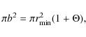
where
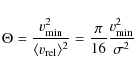
|
(8) |
is the gravitational focusing term or Safronov number, b the impact parameter,
Table 2: Typical stellar encounter parameters.
In summary, the encounter-induced disc-mass loss in cluster
environments of different densities shows two important features:
i) low-mass stars lose a
larger fraction of their disc material with increasing cluster density;
and ii) the discs of the most massive stars are (nearly)
completely destroyed;
regardless of the density of the cluster environment. The important
finding for i) is that the correlation is not linear, but shows a much
larger
increase for the cluster models with higher densities than
model D2, implying that there exists a critical density
![]() that marks the onset of a much more destructive effect of star-disc
encounters. This critical density seems to be close to the density of
the ONC,
that marks the onset of a much more destructive effect of star-disc
encounters. This critical density seems to be close to the density of
the ONC,
![]() .
.
We find that the evolution of the CDF in the Trapezium Cluster region is very similar among the size-scaled models and corresponds to the distribution of the model D2 in Fig. 3. The size-scaled models are obviously of the same importance in their environmental effect on protoplanetary discs despite the slightly different dynamical evolution. The density of the models S0 and S1 decreases faster than for the more massive clusters, even up to a factor of 2 in the case of the model S0 (see Sect. 5.1). Thus one would expect a lower encounter rate in these smaller systems and, consequently, on average a lower disc-mass loss. However, this is obviously not the case and is explained by the fact that, similarly to the finding for the density-scaled models, high-mass stars become less important as gravitational foci for the low-mass stars in clusters with larger stellar populations. Hence in terms of encounter statistics, the lower density of the models S0 and S1 is compensated by the more frequent interactions of the high-mass stars.
5.3 Validation of the numerical method
So far the disc-mass loss has been calculated from the Eq. (1) of Pfalzner et al. (2006)
by treating all encounters as parabolic. To account for the lower
disc-mass loss in hyperbolic encounters, we have determined a function
that quantifies the reduction of the disc-mass loss in dependence of
the orbital eccentricity:
Equation (9) is a fit function to the median distribution of the relative disc-mass loss as a function of eccentricity, adapted to the parabolic case, for all star-disc simulations that have been performed.
![\begin{figure}
\par\includegraphics[angle=-90,width=8cm,clip]{12641f06.eps} \includegraphics[angle=-90,width=8cm,clip]{12641f07.eps}
\vspace*{-2.5mm}
\end{figure}](/articles/aa/full_html/2010/01/aa12641-09/img101.png)
|
Figure 6: Number of encounters as a function of eccentricity (logarithmic bins), plotted for three different groups by means of disc-mass loss per encounter. The white surface represents all encounters (i.e. a minimum of 3% disc-mass loss, cf. Olczak et al. 2006), the light grey surface those that removed at least 50% of the disc-mass, while the dark grey one stands for the most destructive encounters which caused a disc-mass loss of at least 90%. The two plots show the distributions for the model D4. Top: disc-mass loss calculated assuming parabolic encounters. Bottom: disc-mass loss calculation corrected for effects of eccentricity by using Eq. (9). |
| Open with DEXTER | |
As shown in Fig. 6, the number of hyperbolic encounters is significantly reduced if the eccentricity is considered explicitly in the calculation of the disc-mass loss using the fit function (9). This is a consequence of our definition of an encounter (see Sect. 3): the fraction of those perturbations which cause a relative disc-mass loss of above 3% is lower for higher eccentricities, hence the number of eccentric encounters decreases. However, because the fit function represents the median distribution of all simulated star-disc encounters and the effect of strongly perturbing encounters is only weakly dependent on the eccentricity, the number of strongly perturbing encounters in Fig. 6b (light and dark grey surfaces) is underestimated.
![\begin{figure}
\par\includegraphics[angle=-90,width=8cm,clip]{12641f08.eps}
\vspace*{-2mm}
\end{figure}](/articles/aa/full_html/2010/01/aa12641-09/img102.png)
|
Figure 7:
Time evolution of the cluster disc fraction of the density-scaled
models, not restricted to parabolic encounters, for a region of the
size of the Trapezium Cluster (
|
| Open with DEXTER | |
It is accordingly the disc-mass loss induced by weak hyperbolic
interactions that has been overestimated in the calculations. These
events are most
numerous in the models D3-D5 with densities of
![]() and result preferentially from interactions of low-mass stars with
roughly equal-mass perturbers. Consequently, when considering
explicitly the reduced disc-mass loss in hyperbolic encounters (see
Fig. 7), the outstanding role of these dense clusters as environments of huge disc
destruction becomes less pronounced (cf. Fig. 3), though the encounter-induced disc-mass loss is still considerably larger compared to the sparser clusters D0-D2.
and result preferentially from interactions of low-mass stars with
roughly equal-mass perturbers. Consequently, when considering
explicitly the reduced disc-mass loss in hyperbolic encounters (see
Fig. 7), the outstanding role of these dense clusters as environments of huge disc
destruction becomes less pronounced (cf. Fig. 3), though the encounter-induced disc-mass loss is still considerably larger compared to the sparser clusters D0-D2.
![\begin{figure}
\par\includegraphics[angle=-90,width=8cm,clip]{12641f09.eps}
\vspace*{-2mm}
\end{figure}](/articles/aa/full_html/2010/01/aa12641-09/img104.png)
|
Figure 8:
Average relative disc-mass loss at 1 Myr for the Trapezium Cluster
as a function of the stellar mass for initially equal disc sizes. The
standard ONC model with a stellar upper mass limit of 50 |
| Open with DEXTER | |
In Fig. 8
we investigate the effect of the higher upper
mass limit on our results as compared to the basic ONC model. It shows
the average relative disc-mass loss as a function of the stellar mass
for the
standard ONC model with a stellar upper mass limit of 50 ![]() (dark grey boxes), and the same model with an upper mass limit of 150
(dark grey boxes), and the same model with an upper mass limit of 150 ![]() (light
grey boxes). For masses below 10
(light
grey boxes). For masses below 10 ![]() the two distributions are quantitatively in good agreement.
the two distributions are quantitatively in good agreement.
In the range of ![]() 10-50
10-50
![]() the average disc-mass loss of the 50
the average disc-mass loss of the 50
![]() -limit model is significantly higher. This is to be expected because
stars in this mass range can act as additional strong gravitational foci in the presence of a 50
-limit model is significantly higher. This is to be expected because
stars in this mass range can act as additional strong gravitational foci in the presence of a 50
![]() star, while their effect is largely reduced
if a 150
star, while their effect is largely reduced
if a 150
![]() star is gravitationally dominating. The most massive stars in the range
star is gravitationally dominating. The most massive stars in the range
![]() show, as expected, the largest average
relative disc-mass loss. That it is somewhat lower than the one of the most massive star of the 50
show, as expected, the largest average
relative disc-mass loss. That it is somewhat lower than the one of the most massive star of the 50
![]() -limit
model agrees with the stronger
gravitational attraction of their disc, leading on average to a reduced
disc-mass loss per encounter. However, since the highest mass bin is
only
populated by nine stars, any further conclusions about the average
relative disc-mass loss of the most massive stars would be highly
speculative.
-limit
model agrees with the stronger
gravitational attraction of their disc, leading on average to a reduced
disc-mass loss per encounter. However, since the highest mass bin is
only
populated by nine stars, any further conclusions about the average
relative disc-mass loss of the most massive stars would be highly
speculative.
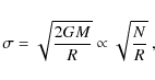
6 Comparison of numerical results and analytical estimates
In this section the numerical results will be compared to analytical
estimates. The treatment of encounters involves one important time
scale, the
collision time
![]() (Binney & Tremaine 1987, Eq. (8-123)),
(Binney & Tremaine 1987, Eq. (8-123)),
![\begin{displaymath}
t_{\rm coll} = \left[ 16 \sqrt{\pi} \rho \sigma r_\star^2 \l...
... + \frac{Gm_\star}{2\sigma^2r_\star}\right) \right]^{-1} \cdot
\end{displaymath}](/articles/aa/full_html/2010/01/aa12641-09/img107.png)
Here the inverse of the collision time will be introduced as the encounter rate,

the encounter rate can be written as
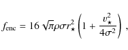
where G denotes the gravitational constant,
where
Because the model D2/S2 represents the standard ONC model, which
has been intensively studied, the calculations will be adapted to this
model. All
quantities related to this model will be denoted accordingly by
a ``0'' as subscript. Adopting the initial velocity dispersion of
the model D2/S2,
![]() ,
using
,
using
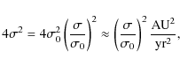
and the numbers given in Table 2, Eq. (12) can be simplified to
![\begin{displaymath}
f_{{\rm enc}} = 16 \sqrt{\pi} \rho \sigma r_{{\rm enc}}^2(m_...
...ar}) \left( \frac{ \sigma_0 }
{\sigma } \right)^2 \right]\cdot
\end{displaymath}](/articles/aa/full_html/2010/01/aa12641-09/img121.png)
An even more compact representation is achieved by considering the scaling properties of the two families of models: as can be derived from Eqs. (4) and (6), the scaling relations for the density-scaled models are
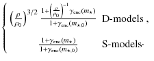
The derived relation for the adapted encounter rate predicts very different scaling relations for the two families of cluster models. Density-scaled models are expected to show large variations of the number of encounters, with a strong dependency on the density for low-mass stars, i.e. when
Table 3: Approximate relative encounters rates.
In summary, what one would expect from the numerical simulations of the
density-scaled models is a steep increase of the encounter rate
![]() in the case of the low-mass stars and a considerably shallower dependency
in the case of the low-mass stars and a considerably shallower dependency
![]() for the high-mass stars. For low densities,
corresponding to low particle numbers, one would expect that the
high-mass stars dominate the encounter rate via gravitational focusing,
favouring an
overall scaling
for the high-mass stars. For low densities,
corresponding to low particle numbers, one would expect that the
high-mass stars dominate the encounter rate via gravitational focusing,
favouring an
overall scaling
![]() .
In contrast, the size-scaled models should produce very similar results in terms of encounter rate, regardless
of the specific cluster model.
.
In contrast, the size-scaled models should produce very similar results in terms of encounter rate, regardless
of the specific cluster model.
![\begin{figure}
\par\includegraphics[angle=-90,width=8cm,clip]{12641f10.eps}\includegraphics[angle=-90,width=8cm,clip]{12641f11.eps}
\end{figure}](/articles/aa/full_html/2010/01/aa12641-09/img140.png)
|
Figure 9:
Normalised encounter rate
|
| Open with DEXTER | |
These expectations agree well with the results from the numerical simulations. We demonstrate this in Fig. 9 by the average encounter rate of stars of all masses and of the three mass groups, respectively, adapted in each case to the model D2/S2. Figure 9a shows that the encounter rates of the cluster models D0-D2 are scaling roughly as N1/2. For higher particle numbers the distribution becomes more complex. Here the high-mass stars show a trend of a decreasing encounter rate with the particle number. This feature accounts for the decreasing importance of the high-mass stars as gravitational foci (for the lower mass stars) and is a consequence of the decreasing ratio of the mass of the most massive star and the cluster mass. Accordingly, the distribution of the encounter rate tends towards the analytical limit of N3/2 for low-mass stars, representing the more frequent interaction of low-mass stars among themselves in the models D3-D5.
Figure 9b shows that the size-scaled models are of the same importance in their environmental effect on protoplanetary discs. In the case of low- and intermediate mass stars the presented encounter rates, adapted to the model S2, agree well with the analytical estimate, which predicts a constant distribution as a function of particle number. In contrast, the adapted encounter rate of the high-mass stars decreases with an increasing particle number. This trend shows that the high-mass stars, similar to the finding for the density-scaled models, become less important as gravitational foci for the low-mass stars in clusters with larger stellar populations.
7 Conclusion and discussion
The influence of different cluster environments on the encounter-induced disc-mass loss has been investigated by scaling the size, density and stellar number of the basic dynamical model of the ONC. The results can be summarised as follows:
- 1.
- The disc-mass loss increases with cluster density but remains unaffected by the size of the stellar population.
- 2.
- The density of the ONC itself marks a threshold:
- (a)
- in less dense and less massive clusters it is the massive stars that dominate the encounter-induced disc-mass loss by a gravitational focusing of low-mass stars, whereas
- (b)
- in denser and more massive clusters the interactions of low-mass stars with equal-mass perturbers play the major role for the removal of disc mass.
- 3.
- In clusters four times sparser than the ONC the effect of encounters is still apparent.
![\begin{figure}
\par\includegraphics[angle=-90,width=8cm,clip]{12641f12.eps}
\end{figure}](/articles/aa/full_html/2010/01/aa12641-09/img145.png)
|
Figure 10:
Cluster density as a function of cluster size for clusters more massive than
|
| Open with DEXTER | |
Our results have several important implications for the general picture of star- and cluster formation. Very recently, Pfalzner (2009) has shown that there two cluster sequences exist, evolving in time along pre-defined tracks in the density-radius plane, the ``leaky'' and the ``star-burst'' clusters. The simulations performed in the present investigation cover the parameter space of the ``leaky'' clusters in their embedded stage (see Fig. 10). A comparison with our results shows that at the earliest evolutionary stage leaky clusters have densities above the critical density. Hence in leaky clusters star-disc systems are initially efficiently destroyed via encounters that occur preferentially between low-mass stars. The ONC corresponds to an intermediate stage in the embedded phase of leaky clusters with the transition towards a preferred disc-mass loss of high-mass stars via gravitational focusing of low-mass stars. At the final stage of the embedded phase the encounter-induced disc-mass loss in leaky clusters ceases. Gravitational focusing by high-mass stars may still affect single objects, yet at this age is most probably exceeded by other disc-destructive processes like photoevaporation or planet formation. The effects in star-burst clusters would be similar, yet much more pronounced. In case of the Arches cluster one could expect stellar encounters to destroy the discs of most of the low- and high-mass stars in several hundred thousand years. Combining our results with those of Lada & Lada (2003) that most stars are born in clusters, it becomes evident that a significant fraction of all stars must have been affected by stellar encounters at the early evolutionary stages of their hosting environment.
The application of our results to the dynamics of embedded clusters - though obtained from simulations that do not contain gas - is justified for three reasons:
- 1.
- Rather than simulating the evolution of leaky clusters (which would explicitly require the treatment of gas), we use our cluster models to map certain evolutionary stages of the sequence of leaky clusters in terms of ``dynamical snapshots''. The dynamical effects of these numerical models are then used to estimate the effect of encounters in the observedclusters at their current dynamical state.
- 2.
- The effect of gas in an embedded cluster is to lower the frequency of close encounters (due to the smoother cluster potential), yet unless the gas mass is dominating cluster dynamics - as is not the case for the only partially embedded leaky clusters shown in Fig. 10 (e.g. NGC 2024) - the effect is minor.
- 3.
- Gas expulsion causes the clusters to expand and thus their density to decrease much faster than in our simulations. Consequently, when mapping our results to the current dynamical state, we underestimate the initial cluster density and thus the effect of encounters in the early evolutionary phases. Hence, our results are least accurate for older clusters, yet well applicable for the young evolutionary stages, where encounters have the most significant effect.
We thank the anonymous referee and the editor for careful reading and very useful comments and suggestions which improved this work. C. Olczak appreciates fruitful discussions with S. Portegies Zwart concerning the analytical estimates and scaling relations. We also thank R. Spurzem for providing the NBODY6++ code for the cluster simulations. Simulations were partly performed at the Jülich Supercomputing Centre (JSC), Research Centre Jülich, Project HKU14. We are grateful for the excellent support by the JSC Dispatch team.
Table A.1: Boundaries of the three mass groups of low-, intermediate-, and high-mass stars of cluster models with 1000, 2000, 4000, 8000, 16 000, and 32 000 particles.
Appendix A: Determination of boundaries of mass groups
Boundaries of mass groups of low-, intermediate- and high-mass stars have been determined individually for different sizes of stellar populations on the basis of the IMF of Kroupa (2001, see also Eq. (1)#. The derivation involves the requirement for the three mass ranges to be equidistant in logarithmic space, weighted by the slope of the IMF (of each mass range). The weighting accounts for the steepness of the slope in the high-mass regime, which would otherwise cause a very sparsely populated group of high-mass stars.
In the case of a lower mass cutoff at
![]() ,
and an upper mass limit m3, the IMF is characterised by just two different slopes,
,
and an upper mass limit m3, the IMF is characterised by just two different slopes,
![]() in the range of
in the range of
![]() ,
and
,
and
![]() in the range of
in the range of
![]() .
Because the break in the
slope of the IMF at the critical mass
.
Because the break in the
slope of the IMF at the critical mass
![]() does not necessarily coincide with one of the boundaries of the mass ranges,
the cases
does not necessarily coincide with one of the boundaries of the mass ranges,
the cases
![]() and
and
![]() have to be differentiated. Though from the theoretical point of view the same
differentiation would be required for the higher mass boundary m2, this is not relevant for the stellar systems in the focus of the present
work. The four mass ranges, mk, k=0,...,3, and the two slopes,
have to be differentiated. Though from the theoretical point of view the same
differentiation would be required for the higher mass boundary m2, this is not relevant for the stellar systems in the focus of the present
work. The four mass ranges, mk, k=0,...,3, and the two slopes, ![]() ,
k=1,2, are then interrelated as follows:
,
k=1,2, are then interrelated as follows:
| (m1 | |||
| (m1 | < | ||
Solving these equations, and substituting
| |
|||
one obtains
| (16) | |||
The choice of the appropriate solution is determined by the upper mass limit m3. For this purpose the ``critical maximum mass''
![\begin{displaymath}m_c^{{\rm max}} = \log^{-1}{\left[ ( 1 + 2 \alpha_{12} ) \log{m_c^{{\rm br}}} - 2 \alpha_{12} \log{m_0} \right]},
\end{displaymath}](/articles/aa/full_html/2010/01/aa12641-09/img194.png)
is estimated from Eq. (A) and
With the given values of the parameters m0,
The derived mass boundaries, mk, k=0,...,3, for each cluster of the families of models are presented in Table A.1.
References
- Aarseth, S. 2003, Gravitational N-body Simulations (Cambridge: Cambridge University Press), 430 [Google Scholar]
- Adams, F. C., Proszkow, E. M., Fatuzzo, M., et al. 2006, ApJ, 641, 504 [NASA ADS] [CrossRef] [Google Scholar]
- Alexander, R. D., Clarke, C. J., & Pringle, J. E. 2005, MNRAS, 358, 283 [NASA ADS] [CrossRef] [Google Scholar]
- Alexander, R. D., Clarke, C. J., & Pringle, J. E. 2006, MNRAS, 369, 229 [NASA ADS] [CrossRef] [Google Scholar]
- Bally, J., Testi, L., Sargent, A., et al. 1998, AJ, 116, 854 [NASA ADS] [CrossRef] [Google Scholar]
- Balog, Z., Muzerolle, J., Rieke, G. H., et al. 2007, ApJ, 660, 1532 [NASA ADS] [CrossRef] [Google Scholar]
- Bik, A., Lenorzer, A., Kaper, L., et al. 2003, A&A, 404, 249 [Google Scholar]
- Binney, J., & Tremaine, S. 1987, Galactic dynamics (Princeton, NJ: Princeton University Press), 747 [Google Scholar]
- Clarke, C. J., & Pringle, J. E. 1993, MNRAS, 261, 190 [NASA ADS] [CrossRef] [Google Scholar]
- Clarke, C. J., Bonnell, I. A., & Hillenbrand, L. A. 2000, Protostars and Planets IV, 151 [Google Scholar]
- Clarke, C. J., Gendrin, A., & Sotomayor, M. 2001, MNRAS, 328, 485 [NASA ADS] [CrossRef] [Google Scholar]
- Currie, T., Kenyon, S. J., Balog, Z., et al. 2008, ApJ, 672, 558 [Google Scholar]
- de Pree, C. G., Nysewander, M. C., & Goss, W. M. 1999, AJ, 117, 2902 [NASA ADS] [CrossRef] [Google Scholar]
- Drake, J. J., Ercolano, B., Flaccomio, E., et al. 2009, ApJ, 699, L35 [NASA ADS] [CrossRef] [Google Scholar]
- Ercolano, B., Drake, J. J., Raymond, J. C., et al. 2008, ApJ, 688, 398 [NASA ADS] [CrossRef] [Google Scholar]
- Falgarone, E., & Phillips, T. G. 1990, ApJ, 359, 344 [NASA ADS] [CrossRef] [PubMed] [Google Scholar]
- Figer, D. F. 2005, Nature, 434, 192 [NASA ADS] [CrossRef] [PubMed] [Google Scholar]
- Gorti, U., & Hollenbach, D. 2009, ApJ, 690, 1539 [Google Scholar]
- Haisch, K. E., Lada, E. A., & Lada, C. J. 2000, AJ, 120, 1396 [NASA ADS] [CrossRef] [Google Scholar]
- Haisch, Jr., K. E., Lada, E. A., & Lada, C. J. 2001, ApJ, 553, L153 [NASA ADS] [CrossRef] [Google Scholar]
- Hall, S. M. 1997, MNRAS, 287, 148 [NASA ADS] [CrossRef] [Google Scholar]
- Hall, S. M., Clarke, C. J., & Pringle, J. E. 1996, MNRAS, 278, 303 [NASA ADS] [Google Scholar]
- Heller, C. H. 1993, ApJ, 408, 337 [NASA ADS] [CrossRef] [Google Scholar]
- Heller, C. H. 1995, ApJ, 455, 252 [NASA ADS] [CrossRef] [Google Scholar]
- Hillenbrand, L. A. 1997, AJ, 113, 1733 [NASA ADS] [CrossRef] [Google Scholar]
- Hillenbrand, L. A. 2002 [arXiv:0210520] [Google Scholar]
- Hillenbrand, L. A. 2005 [arXiv:0511083] [Google Scholar]
- Hillenbrand, L. A., & Carpenter, J. M. 2000, ApJ, 540, 236 [NASA ADS] [CrossRef] [Google Scholar]
- Hillenbrand, L. A., & Hartmann, L. W. 1998, ApJ, 492, 540 [NASA ADS] [CrossRef] [Google Scholar]
- Hillenbrand, L. A., Strom, S. E., Calvet, N., et al. 1998, AJ, 116, 1816 [NASA ADS] [CrossRef] [Google Scholar]
- Hollenbach, D. J., Yorke, H. W., & Johnstone, D. 2000, Protostars and Planets IV, 401 [Google Scholar]
- Johnstone, D., Hollenbach, D., & Bally, J. 1998, ApJ, 499, 758 [NASA ADS] [CrossRef] [Google Scholar]
- Johnstone, D., Matsuyama, I., McCarthy, I. G., et al. 2004, in Rev. Mex. Astron. Astrofis. Conf. Ser. 22, ed. G. Garcia-Segura, G. Tenorio-Tagle, J. Franco, & H. W. Yorke, 38 [Google Scholar]
- Kley, W., Papaloizou, J. C. B., & Ogilvie, G. I. 2008, A&A, 487, 671 [Google Scholar]
- Koen, C. 2006, MNRAS, 365, 590 [NASA ADS] [CrossRef] [Google Scholar]
- Kroupa, P. 2001, MNRAS, 322, 231 [NASA ADS] [CrossRef] [Google Scholar]
- Kroupa, P. 2002, Science, 295, 82 [NASA ADS] [CrossRef] [PubMed] [Google Scholar]
- Lada, C. J., & Lada, E. A. 2003, ARA&A, 41, 57 [Google Scholar]
- Lada, C. J., Muench, A. A., Haisch, Jr., K. E., et al. 2000, AJ, 120, 3162 [NASA ADS] [CrossRef] [Google Scholar]
- Larson, R. B. 2003, in Galactic Star Formation Across the Stellar Mass Spectrum, ed. J. M. De Buizer, & N. S. van der Bliek, ASP Conf. Ser., 287, 65 [Google Scholar]
- Liu, W. M., Meyer, M. R., Cotera, A. S., et al. 2003, AJ, 126, 1665 [NASA ADS] [CrossRef] [Google Scholar]
- Luhman, K. L., Rieke, G. H., Young, E. T., et al. 2000, ApJ, 540, 1016 [Google Scholar]
- Maíz Apellániz, J., Walborn, N. R., Morrell, N. I., Niemela, V. S., & Nelan, E. P. 2007, ApJ, 660, 1480 [NASA ADS] [CrossRef] [Google Scholar]
- Mann, R. K., & Williams, J. P. 2009, ApJ, 699, L55 [NASA ADS] [CrossRef] [Google Scholar]
- Maschberger, T., & Clarke, C. J. 2008, MNRAS, 391, 711 [NASA ADS] [CrossRef] [Google Scholar]
- Matsuyama, I., Johnstone, D., & Hartmann, L. 2003, ApJ, 582, 893 [NASA ADS] [CrossRef] [Google Scholar]
- McCaughrean, M., Zinnecker, H., Andersen, M., Meeus, G., & Lodieu, N. 2002, The Messenger, 109, 28 [NASA ADS] [Google Scholar]
- Miesch, M. S., & Scalo, J. M. 1995, ApJ, 450, L27 [NASA ADS] [CrossRef] [Google Scholar]
- Moeckel, N., & Bally, J. 2006, ApJ, 653, 437 [NASA ADS] [CrossRef] [Google Scholar]
- Moeckel, N., & Bally, J. 2007a, ApJ, 661, L183 [NASA ADS] [CrossRef] [Google Scholar]
- Moeckel, N., & Bally, J. 2007b, ApJ, 656, 275 [NASA ADS] [CrossRef] [Google Scholar]
- Muench, A. A., Lada, E. A., Lada, C. J., et al. 2002, ApJ, 573, 366 [NASA ADS] [CrossRef] [Google Scholar]
- Oey, M. S., & Clarke, C. J. 2005, ApJ, 620, L43 [NASA ADS] [CrossRef] [Google Scholar]
- Olczak, C., Pfalzner, S., & Eckart, A. 2008, A&A, 488, 191 [Google Scholar]
- Olczak, C., Pfalzner, S., & Spurzem, R. 2006, ApJ, 642, 1140 [NASA ADS] [CrossRef] [Google Scholar]
- Ostriker, E. C. 1994, ApJ, 424, 292 [NASA ADS] [CrossRef] [Google Scholar]
- Palla, F., & Stahler, S. W. 2000, ApJ, 540, 255 [NASA ADS] [CrossRef] [Google Scholar]
- Pfalzner, S. 2004, ApJ, 602, 356 [NASA ADS] [CrossRef] [Google Scholar]
- Pfalzner, S. 2006, ApJ, 652, L129 [NASA ADS] [CrossRef] [Google Scholar]
- Pfalzner, S. 2009, A&A, 498, L37 [Google Scholar]
- Pfalzner, S., & Olczak, C. 2007a, A&A, 462, 193 [Google Scholar]
- Pfalzner, S., & Olczak, C. 2007b, A&A, 475, 875 [Google Scholar]
- Pfalzner, S., Umbreit, S., & Henning, T. 2005, ApJ, 629, 526 [NASA ADS] [CrossRef] [Google Scholar]
- Pfalzner, S., Olczak, C., & Eckart, A. 2006, A&A, 454, 811 [Google Scholar]
- Pfalzner, S., Tackenberg, J., & Steinhausen, M. 2008, A&A, 487, L45 [Google Scholar]
- Scally, A., & Clarke, C. 2001, MNRAS, 325, 449 [Google Scholar]
- Scally, A., Clarke, C., & McCaughrean, M. J. 2005, MNRAS, 358, 742 [NASA ADS] [CrossRef] [Google Scholar]
- Sicilia-Aguilar, A., Hartmann, L., Calvet, N., et al. 2006, ApJ, 638, 897 [NASA ADS] [CrossRef] [Google Scholar]
- Slesnick, C. L., Hillenbrand, L. A., & Carpenter, J. M. 2004, ApJ, 610, 1045 [NASA ADS] [CrossRef] [Google Scholar]
- Spurzem, R. 1999, J. Comput. Appl. Math., 109, 407 [NASA ADS] [CrossRef] [Google Scholar]
- Stolte, A., Brandner, W., Brandl, B., Zinnecker, H., & Grebel, E. K. 2004, AJ, 128, 765 [NASA ADS] [CrossRef] [Google Scholar]
- Stolte, A., Brandner, W., Brandl, B., et al. 2006, AJ, 132, 253 [NASA ADS] [CrossRef] [Google Scholar]
- Störzer, H., & Hollenbach, D. 1999, ApJ, 515, 669 [CrossRef] [Google Scholar]
- Weidner, C., & Kroupa, P. 2006, MNRAS, 365, 1333 [NASA ADS] [CrossRef] [Google Scholar]
- Williams, J. P., Andrews, S. M., & Wilner, D. J. 2005, ApJ, 634, 495 [NASA ADS] [CrossRef] [Google Scholar]
- Zinnecker, H., & Yorke, H. W. 2007, ARA&A, 45, 481 [Google Scholar]
Footnotes
All Tables
Table 1: Averaged initial parameters of the two families of cluster models.
Table 2: Typical stellar encounter parameters.
Table 3: Approximate relative encounters rates.
Table A.1: Boundaries of the three mass groups of low-, intermediate-, and high-mass stars of cluster models with 1000, 2000, 4000, 8000, 16 000, and 32 000 particles.
All Figures
|
|
Figure 1: Projected density profiles of the density-scaled models compared to observational data. The initial profile (grey lines) and the profile at a simulation time of 1 Myr (black lines) are shown. From bottom to top the cluster models D0-D5 are marked in each colour regime by a short-dashed, long-dashed, solid, dotted, dot-long-dashed, and dot-short-dashed line, respectively. The observational data are from a compilation of McCaughrean et al. (2002) and Hillenbrand (1997). |
| Open with DEXTER | |
| In the text | |
|
|
Figure 2:
Time evolution of stellar densities
|
| Open with DEXTER | |
| In the text | |
|
|
Figure 3:
Time evolution of the cluster disc fraction of the density-scaled models for a region of the size of the Trapezium Cluster
(
|
| Open with DEXTER | |
| In the text | |
|
|
Figure 4: Comparison of the fraction of encounters as a function of the relative perturber mass, i.e. the mass ratio of perturber and perturbed star, of the group of low-mass stars (see Appendix A for the width of the mass intervals) for the models D0 (dotted), D2 (solid), and D4 (dot-long-dashed), respectively. Here initially equal disc sizes have beenassumed. |
| Open with DEXTER | |
| In the text | |
|
|
Figure 5: Comparison of the fraction of encounters as a function of eccentricity of the group of low-mass stars (see Appendix A for the width of the mass intervals) for the models D0 (dotted), D2 (solid), and D4 (dot-long-dashed), respectively. Here initially equal disc sizes have beenassumed. |
| Open with DEXTER | |
| In the text | |
|
|
Figure 6: Number of encounters as a function of eccentricity (logarithmic bins), plotted for three different groups by means of disc-mass loss per encounter. The white surface represents all encounters (i.e. a minimum of 3% disc-mass loss, cf. Olczak et al. 2006), the light grey surface those that removed at least 50% of the disc-mass, while the dark grey one stands for the most destructive encounters which caused a disc-mass loss of at least 90%. The two plots show the distributions for the model D4. Top: disc-mass loss calculated assuming parabolic encounters. Bottom: disc-mass loss calculation corrected for effects of eccentricity by using Eq. (9). |
| Open with DEXTER | |
| In the text | |
|
|
Figure 7:
Time evolution of the cluster disc fraction of the density-scaled
models, not restricted to parabolic encounters, for a region of the
size of the Trapezium Cluster (
|
| Open with DEXTER | |
| In the text | |
|
|
Figure 8:
Average relative disc-mass loss at 1 Myr for the Trapezium Cluster
as a function of the stellar mass for initially equal disc sizes. The
standard ONC model with a stellar upper mass limit of 50 |
| Open with DEXTER | |
| In the text | |
|
|
Figure 9:
Normalised encounter rate
|
| Open with DEXTER | |
| In the text | |
|
|
Figure 10:
Cluster density as a function of cluster size for clusters more massive than
|
| Open with DEXTER | |
| In the text | |
Copyright ESO 2010
Current usage metrics show cumulative count of Article Views (full-text article views including HTML views, PDF and ePub downloads, according to the available data) and Abstracts Views on Vision4Press platform.
Data correspond to usage on the plateform after 2015. The current usage metrics is available 48-96 hours after online publication and is updated daily on week days.
Initial download of the metrics may take a while.