| Issue |
A&A
Volume 509, January 2010
|
|
|---|---|---|
| Article Number | A101 | |
| Number of page(s) | 9 | |
| Section | Stellar atmospheres | |
| DOI | https://doi.org/10.1051/0004-6361/200912434 | |
| Published online | 26 January 2010 | |
The outer atmospheric layers of the early M dwarf Gliese 1
E. Lexen1 - R. Wehrse1,2 - J. Liebert3 - M. S. Bessell4
1 - Institut für Theoretische Astrophysik, Zentrum für Astronomie der Universität Heidelberg,
Albert-Ueberle-Str. 2, 69120 Heidelberg, Germany
2 -
Interdisziplinäres Zentrum für
Wissenschaftliches Rechnen (IWR),
Im Neuenheimer Feld 368, 69120 Heidelberg, Germany
3 -
Steward Observatory, Univ. of Arizona, Tucson, AZ 85721, USA
4 -
RSAA, College of Science, The Australian National University, Cotter Road , Weston Creek ACT 2611, Australia
Received 6 May 2009 / Accepted 5 October 2009
Abstract
Using infrared and high-resolution optical observations of the
M dwarf Gliese 1, we investigated the temperatures in the
upper atmospheric layers of this star with low atmospheric activity. To
fit the H![]() and metal line profiles, the normal radiative equilibrium temperature decrease must be truncated at about log
and metal line profiles, the normal radiative equilibrium temperature decrease must be truncated at about log
![]() above which a steep chromospheric (
above which a steep chromospheric (
![]() K)
rise must be imposed. Unfortunately, the position of the onset of the
chromosphere depends to some extent on the temperature distribution in
the inner parts of the photosphere. The chromosphere is just not
sufficiently optically thick to be seen in the infrared up to
K)
rise must be imposed. Unfortunately, the position of the onset of the
chromosphere depends to some extent on the temperature distribution in
the inner parts of the photosphere. The chromosphere is just not
sufficiently optically thick to be seen in the infrared up to ![]() 30
30 ![]() m. The persistent strength of the TiO bands leads us to check for indications of surface inhomogeneities with negative results.
m. The persistent strength of the TiO bands leads us to check for indications of surface inhomogeneities with negative results.
Key words: stars: atmospheres - stars: chromospheres - stars: late-type - stars: low-mass - stars: fundamental parameters
1 Introduction
M dwarfs are the most numerous stars (70%) in the Milky Way. Even
though they contribute about 40% to the total mass of the stellar
contents, their atmospheres are still poorly understood due to the
myriads of atomic and molecular lines, efficient convection that
reaches very shallow layers, and strong chromospheres and coronae.
Although model atmospheres have been used with increasing success to
model the spectra of M dwarfs in recent years
(Gustafsson et al. 2003; Brett & Plez 1993; Hauschildt et al. 1999; Allard 1990; Gustafsson et al. 2008; Mould 1976,1975),
uncertainties, particularly
in the opacity data and in the modeling of nonradiative fluxes have
up to now inhibited an accurate theoretical determination of the
temperature distribution in the outer layers. Generally, the model
atmosphere/synthetic spectra fits have emphasized the overall energy
distributions and the molecular bands, with little attention paid to the
profiles of atomic lines that are very sensitive to the outer layers.
It is clear that a temperature inversion takes place at the top of the
normal atmosphere in M dwarfs that show evidence of chromospheric
activity, that is, emission lines of H![]() and/or Ca II. However, many
M dwarfs, especially those with kinematics that suggest they are very old,
show little or no evidence of overt chromospheric activity.
and/or Ca II. However, many
M dwarfs, especially those with kinematics that suggest they are very old,
show little or no evidence of overt chromospheric activity.
Golimowski et al. (2004)
present M band photometry for many dwarfs; however, only a few of the
brightest M dwarfs have been observed spectroscopically in the M and N
bands. In this paper, we report (in Sect. 2) observations of the M
dwarf Gliese 1
(Gl 1)
with the ISOPHOT spectrophotometer (Lemke et al. 1996) of the Infrared Space Observatory
(ISO) in the wavelength range 2.5-12.5 ![]() m and the
InfraRed Spectrograph (IRS) on the Spitzer Space Telescope (Houck et al. 2004) in the wavelength range 5.3-38
m and the
InfraRed Spectrograph (IRS) on the Spitzer Space Telescope (Houck et al. 2004) in the wavelength range 5.3-38 ![]() m.
These ISO and Spitzer observations are discussed in Sect. 3.
In Sect. 2, medium and high-dispersion optical spectrophotometry
of Gl 1 are also reported, while in Sect. 4 we attempt empirical
determinations of the vertical temperature distribution of Gl 1 and show that
the observed spectra do show evidence of chromospheric reversals.
The summary discussion is given in Sect. 5.
m.
These ISO and Spitzer observations are discussed in Sect. 3.
In Sect. 2, medium and high-dispersion optical spectrophotometry
of Gl 1 are also reported, while in Sect. 4 we attempt empirical
determinations of the vertical temperature distribution of Gl 1 and show that
the observed spectra do show evidence of chromospheric reversals.
The summary discussion is given in Sect. 5.
2 Observations
2.1 Parameters of the observed star
The star targeted for ISO and Spitzer observations provides ideal tests of
the hypothesis that even inactive M dwarfs may retain chromospheric
temperature reversals.
Table 1 includes some relevant parameters and data for the target. It is
noteworthy that Gl 1 is a dM star known to lack
H![]() emission, one sign of an active chromosphere. It shows old
disk or halo kinematics. Eggen (1979) classified Gl 1 as old disk whereas
Leggett (1992) and
Leggett & Hawkins (1988) classified Gl 1 as a halo star
noting that it is subluminous in an MI I-K color magnitude diagram,
the signature of a metal-poor, Pop II M subdwarf.
Gl 1 has an age of many Gyr, whether it is from the old disk or halo population.
It has a slight metal deficiency in accordance with its space motion and
it is probably massive enough to possess a small
radiative core. Thus, it should be an example of a star in which a normal magnetic
dynamo has had time to spin down the star. To our knowledge, direct
measurements of the rotation (
emission, one sign of an active chromosphere. It shows old
disk or halo kinematics. Eggen (1979) classified Gl 1 as old disk whereas
Leggett (1992) and
Leggett & Hawkins (1988) classified Gl 1 as a halo star
noting that it is subluminous in an MI I-K color magnitude diagram,
the signature of a metal-poor, Pop II M subdwarf.
Gl 1 has an age of many Gyr, whether it is from the old disk or halo population.
It has a slight metal deficiency in accordance with its space motion and
it is probably massive enough to possess a small
radiative core. Thus, it should be an example of a star in which a normal magnetic
dynamo has had time to spin down the star. To our knowledge, direct
measurements of the rotation (
![]() )
are not available, since
the star is generally too far south for the survey of Gliese stars
by Stauffer & Hartmann (1986).
In the literature, the spectral type of Gl 1 ranges from M1.5V (Hawley et al. 1996; Cincunegui & Mauas 2004) to M4V (Gliese 1969; Evans 1961).
The spectral type would be close to M2V from R-I and V-I whereas B-V is slightly bluer than an M2V star and implies M1V (Bessell 1991; Reid & Hawley 2000).
It is more physically realistic to use the red R-I or V-I color rather than the blue B-V color (Bessell 1990).
Using the TiO5 bandstrengths as suggested in Hawley et al. (1996) indicates it is close to M1.5V.
)
are not available, since
the star is generally too far south for the survey of Gliese stars
by Stauffer & Hartmann (1986).
In the literature, the spectral type of Gl 1 ranges from M1.5V (Hawley et al. 1996; Cincunegui & Mauas 2004) to M4V (Gliese 1969; Evans 1961).
The spectral type would be close to M2V from R-I and V-I whereas B-V is slightly bluer than an M2V star and implies M1V (Bessell 1991; Reid & Hawley 2000).
It is more physically realistic to use the red R-I or V-I color rather than the blue B-V color (Bessell 1990).
Using the TiO5 bandstrengths as suggested in Hawley et al. (1996) indicates it is close to M1.5V.
2.2 ISOPHOT and IRS
Table 1: Relevant parameters of Gl 1.
|
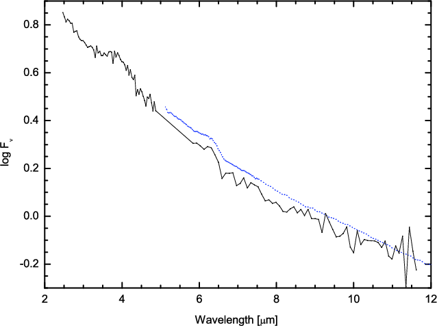
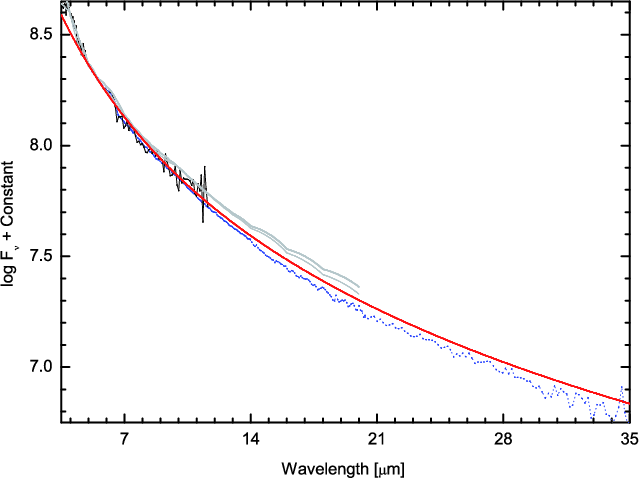
Figure 1: ISOPHOT S (solid line) and IRS (dotted line) flux distributions for Gl 1. |
| Open with DEXTER | |
|
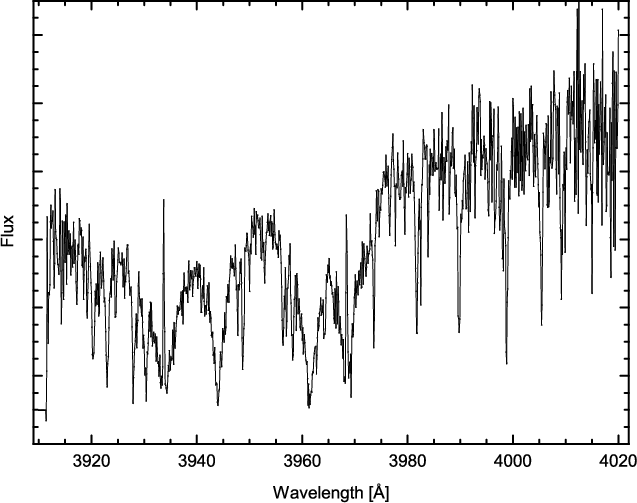
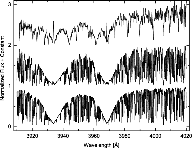
Figure 2: The spectrum of Gl 1 in the range of 3910-4020 Å around the Ca II H and K lines with a resolution of 100 mÅ. Note the strong but very narrow emission in the cores of Ca II K (3933.7 Å) and Ca II H (3968.5 Å). |
| Open with DEXTER | |
|
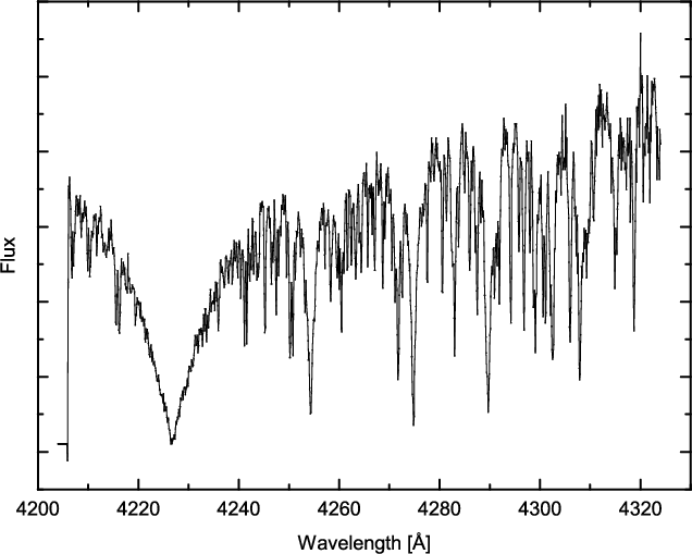
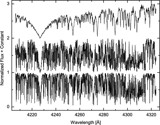
Figure 3: The spectrum of Gl 1 in the range of 4206-4324 Å around the Ca I line with a resolution of 100 mÅ. |
| Open with DEXTER | |
2.3 Mt. Stromlo and Siding Spring spectrophotometry
In order to investigate further the properties of this ISO and Spitzer target - in particular, to determine from line profiles whether they show any evidence of chromospheric activity or non-LTE effects - spectra were obtained in June 2007 with the Boller & Chivens grating cross dispersed echelle spectrograph on the Nasmyth B focus on the 2.3 m reflector at Siding Spring Observatories. A 79 g/mm echelle grating with dispersion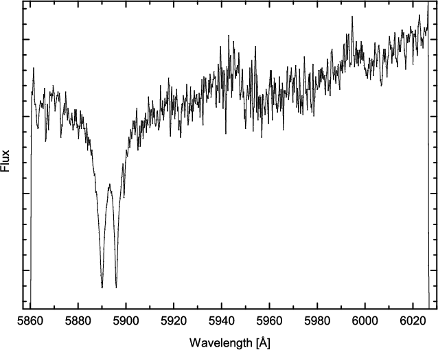
|
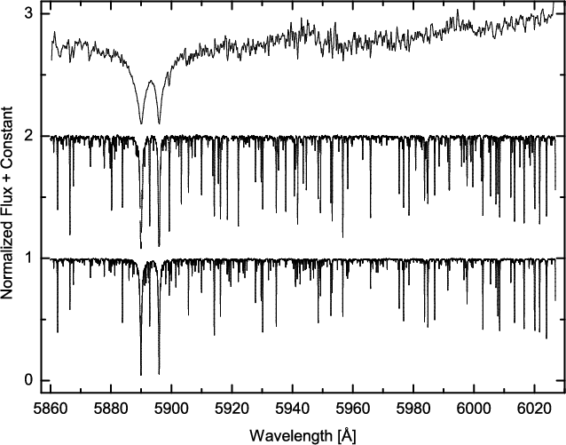
Figure 4: The spectrum of Gl 1 in the range of 5860-6027 Å around the Na I D2 and D1 lines with a resolution of 200 mÅ. |
| Open with DEXTER | |
|
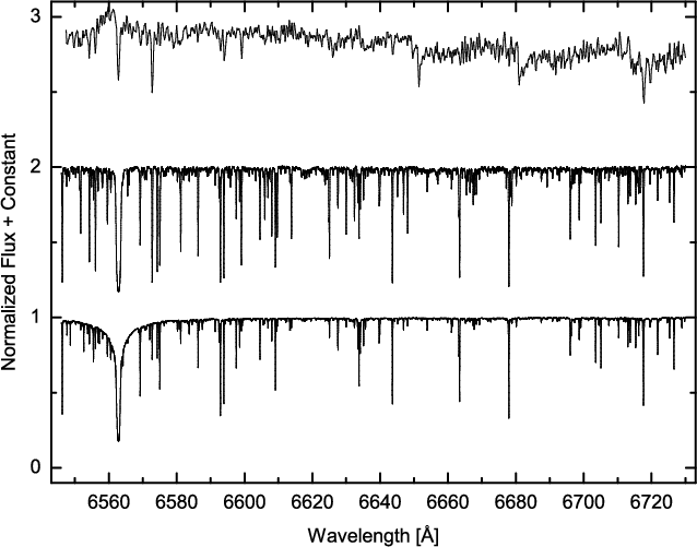
Figure 5:
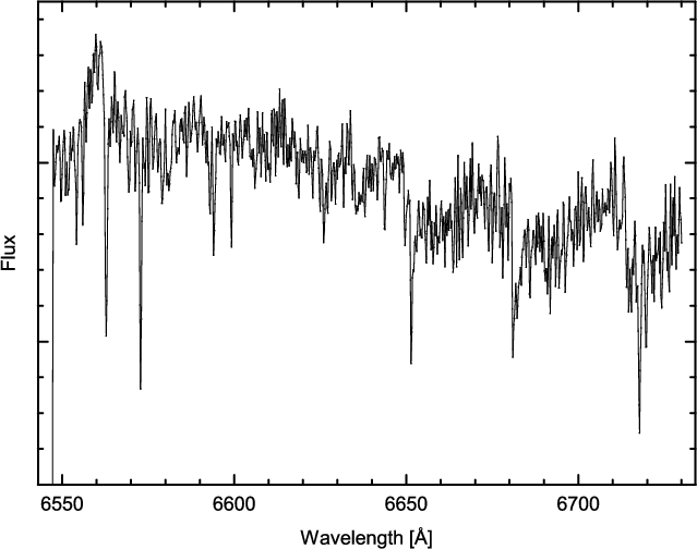
The spectrum of Gl 1 in the range of 6546-6730 Å around the H |
| Open with DEXTER | |
|
Figure 6: The spectra of the stars Gl 1 (M1.5), Arcturus (K1.5) and the Sun (G2) from top to bottom in the range of 3910-4020 Å around the Ca II H and K lines. |
| Open with DEXTER | |
|
Figure 7: The spectra of the stars Gl 1 (M1.5), Arcturus (K1.5) and the Sun (G2) from top to bottom in the range of 4206-4324 Å around the Ca I line. |
| Open with DEXTER | |
|
Figure 8: The spectra of the stars Gl 1 (M1.5), Arcturus (K1.5) and the Sun (G2) from top to bottom in the range of 5860-6027 Å around the Na I D lines. |
| Open with DEXTER | |
|
Figure 9:
The spectra of the stars Gl 1 (M1.5), Arcturus (K1.5) and the Sun
(G2) from top to bottom in the range of 6546-6730 Å around the H |
| Open with DEXTER | |
|
Figure 10:
Flux distributions for Gl 1 as shown in Fig. 1 in
the range 3.5-35 |
| Open with DEXTER | |
|
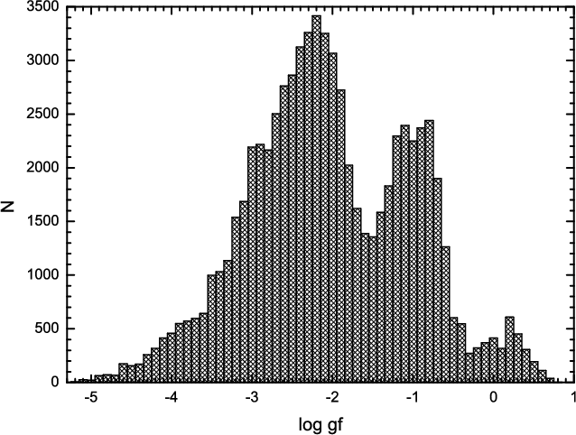
Figure 11: Distribution of the numbers of titanium oxide lines (Plez 1998) used in the modeling of the spectrum in the wavelength range 6550-6580 Å as a function of the gf-values of the lines. It is seen that there are essentially three peaks but the distributions are essentially continuous. |
| Open with DEXTER | |
|
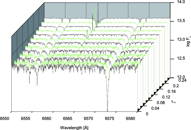
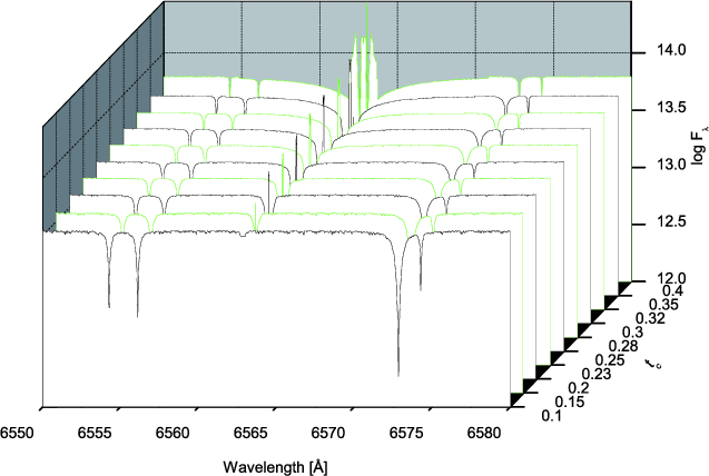
Figure 12:
Model series with gray temperature stratification for
|
| Open with DEXTER | |

|
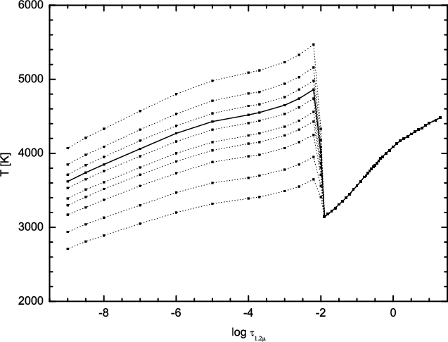
Figure 13:
Temperature as a function of the optical depth at |
| Open with DEXTER | |
|
Figure 14:
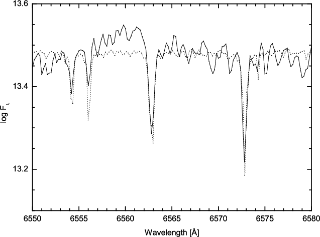
Comparison of high resolution observations of Gl 1 (full line) and
synthetic spectra calculated with an additional cool chromosphere with
parameters
|
| Open with DEXTER | |
|
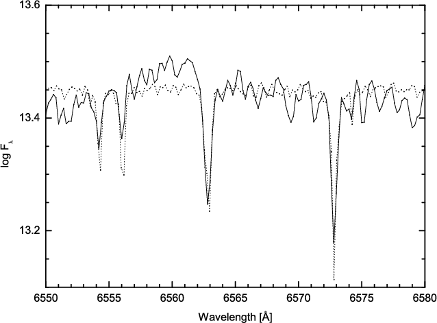
Figure 15:
Same as Fig. 14 but for parameters
|
| Open with DEXTER | |
3 Infrared flux distribution
In Fig. 10 is shown the observed ISOPHOT S (solid line) and IRS
fluxes (dotted line) (shifted by an additional constant) compared with
the distribution of a black body of
![]() K and
two calculated models with and without an additional cool
chromosphere. The temperature stratification for the model with an
additional component is shown in Fig. 18 (full line).
K and
two calculated models with and without an additional cool
chromosphere. The temperature stratification for the model with an
additional component is shown in Fig. 18 (full line).
4 Interpretation of the line profiles
The obtained optical spectra of the M 1.5V dwarf Gl 1 (Figs. 2-5) was compared with the spectra of the red giant Arcturus (![]() Boo) (K1.5 III) and the Sun (G2V) (Figs. 6-9). The resolution of the spectra of Gl 1 are inferior to the others. The spectra of Arcturus (Hinkle et al. 2000) and the Sun (Kurucz 2005)
are freely available on the web. For our purpose the spectrum of
Arcturus has been corrected for negative values that were introduced by
the observer for regions with poorly corrected telluric absorption
features and for regions that were suspected to be affected by detector
blemishes. Note that the very different appearances of the Ca II H
and K lines of these objects reflect to a large extent the very
different line blanketing. Furthermore, the emission components in the
H and K lines (Fig. 6)
reflect differences in the chromospheres. It is seen that in the dwarf
Gl 1 very few lines and weak band heads can be identified and
other lines form a quasi-continuum in the spectral range
6546-6730 Å (Fig. 9).
A close look at the spectra of Gl 1 shows that several profiles of strong lines in the high dispersion optical
and far-red spectra indicate deviations from the radiative
equilibrium temperature distribution and from LTE level occupations
in the top layers of the atmosphere:
Fig. 2 shows evidence for reversals of the Ca II resonance line
cores. The emission cores for the early
objects require a reversal in the temperature in the top layers for at
least some part of the photospheric disk.
Boo) (K1.5 III) and the Sun (G2V) (Figs. 6-9). The resolution of the spectra of Gl 1 are inferior to the others. The spectra of Arcturus (Hinkle et al. 2000) and the Sun (Kurucz 2005)
are freely available on the web. For our purpose the spectrum of
Arcturus has been corrected for negative values that were introduced by
the observer for regions with poorly corrected telluric absorption
features and for regions that were suspected to be affected by detector
blemishes. Note that the very different appearances of the Ca II H
and K lines of these objects reflect to a large extent the very
different line blanketing. Furthermore, the emission components in the
H and K lines (Fig. 6)
reflect differences in the chromospheres. It is seen that in the dwarf
Gl 1 very few lines and weak band heads can be identified and
other lines form a quasi-continuum in the spectral range
6546-6730 Å (Fig. 9).
A close look at the spectra of Gl 1 shows that several profiles of strong lines in the high dispersion optical
and far-red spectra indicate deviations from the radiative
equilibrium temperature distribution and from LTE level occupations
in the top layers of the atmosphere:
Fig. 2 shows evidence for reversals of the Ca II resonance line
cores. The emission cores for the early
objects require a reversal in the temperature in the top layers for at
least some part of the photospheric disk.
A spectrum covering the H![]() line is shown for Gl 1 in
Fig. 5.
Also seen in the spectral region of Fig. 5 is the
strong Ca I line at 6572.795 Å, lines of Ti I 6554.298 and 6556.077 Å,
and numerous weak TiO absorption features across the spectra.
H
line is shown for Gl 1 in
Fig. 5.
Also seen in the spectral region of Fig. 5 is the
strong Ca I line at 6572.795 Å, lines of Ti I 6554.298 and 6556.077 Å,
and numerous weak TiO absorption features across the spectra.
H![]() is seen strongly in absorption in Gl 1. With an equivalent width of -0.39 Å
and
R-I = 1.15 (Robinson et al. 1990), Gl 1 falls
near the bottom of the envelope of M dwarfs of similar color in Fig. 3
of Stauffer & Hartmann (1986), Fig. 6 of Gizis et al. (2002) and Fig. 7 of Robinson et al. (1990).
is seen strongly in absorption in Gl 1. With an equivalent width of -0.39 Å
and
R-I = 1.15 (Robinson et al. 1990), Gl 1 falls
near the bottom of the envelope of M dwarfs of similar color in Fig. 3
of Stauffer & Hartmann (1986), Fig. 6 of Gizis et al. (2002) and Fig. 7 of Robinson et al. (1990).
The n = 2 lower level of hydrogen has an excitation potential of
10.2 eV. For a simple atmosphere in radiative equilibrium at the
indicated temperature near 3600 K, the corresponding Boltzmann factor
would be smaller than 10-17 and no H![]() absorption should
appear. Instead, it is necessary to assume that the line is actually
formed in hotter, outer layers and is subject to strong NLTE effects
that reduce the source function. These findings are in accordance with
the calculations of Cram & Mullan (1979), Houdebine et al. (1995) and Short & Doyle (1997) and
others; these show that the first effect of a weak chromospheric
reversal in the outer atmospheric layers is to produce a pure absorption
line. As the reversal becomes stronger, the line gets weaker, then
finally goes into emission. Empirical evidence in favor of this
interpretation is discussed by Stauffer & Hartmann (1986).
The strength of the absorption
actually indicates a weak chromosphere compared with stars of similar colors (Fig. 14) in the Stauffer & Hartmann (1986) sample, because the absorptions are stronger than
the average. Cram & Mullan (1979) calculated for an atmospheric
absorption should
appear. Instead, it is necessary to assume that the line is actually
formed in hotter, outer layers and is subject to strong NLTE effects
that reduce the source function. These findings are in accordance with
the calculations of Cram & Mullan (1979), Houdebine et al. (1995) and Short & Doyle (1997) and
others; these show that the first effect of a weak chromospheric
reversal in the outer atmospheric layers is to produce a pure absorption
line. As the reversal becomes stronger, the line gets weaker, then
finally goes into emission. Empirical evidence in favor of this
interpretation is discussed by Stauffer & Hartmann (1986).
The strength of the absorption
actually indicates a weak chromosphere compared with stars of similar colors (Fig. 14) in the Stauffer & Hartmann (1986) sample, because the absorptions are stronger than
the average. Cram & Mullan (1979) calculated for an atmospheric
![]() of 3500 K that the maximum absorption equivalent width
would be -0.69 Å, of which only -0.08 Å is caused by the normal
photosphere. Gl 1 has an equivalent width of -0.39 Å (Panagi & Mathioudakis 1993; Robinson et al. 1990).
The neighboring Ca I resonance line (6572 Å) is deeper than expected
from a radiative equilibrium atmosphere. We suspect therefore that it
is also formed in ``scattering mode''. It is very narrow, implying that
the microturbulence plus rotational velocity is quite low.
The spectra certainly require a full NLTE analysis. Unfortunately, a
corresponding program is presently not available to us.
of 3500 K that the maximum absorption equivalent width
would be -0.69 Å, of which only -0.08 Å is caused by the normal
photosphere. Gl 1 has an equivalent width of -0.39 Å (Panagi & Mathioudakis 1993; Robinson et al. 1990).
The neighboring Ca I resonance line (6572 Å) is deeper than expected
from a radiative equilibrium atmosphere. We suspect therefore that it
is also formed in ``scattering mode''. It is very narrow, implying that
the microturbulence plus rotational velocity is quite low.
The spectra certainly require a full NLTE analysis. Unfortunately, a
corresponding program is presently not available to us.
![\begin{figure}
\par\includegraphics[width=17cm]{12434f16.eps}
\end{figure}](/articles/aa/full_html/2010/01/aa12434-09/img52.png)
|
Figure 16:
Synthetic spectra calculated with an additional cool chromosphere including convection with
|
| Open with DEXTER | |
![\begin{figure}
\par\includegraphics[width=17cm]{12434f17.eps}
\end{figure}](/articles/aa/full_html/2010/01/aa12434-09/img58.png)
|
Figure 17:
Same as Fig. 16 but for parameters
|
| Open with DEXTER | |
From these comparisons we see that:
- (i)
- without an outer temperature rise the molecular lines are
reasonably well reproduced. A large fraction of the discrepancies most
probably result from uncertainties in the TiO line data as comparisons
with Kurucz's and Joergensen's list have shown, but the atomic lines
do not fit at all; in particular, H
 absorption is completely
absent, as expected from the cited earlier papers;
absorption is completely
absent, as expected from the cited earlier papers;
- (ii)
- with an increasing temperature rise, the atomic lines fit reasonably well but now the molecular features are too weak;
- (iii)
- the predicted H line is completely absent without an outer temperature rise. With a temperature rise, H
starts with an increasing absorption component, finally superimposed
with a very narrow emission core that is not observed. We therefore
modified the temperature distribution in various ways to avoid the
emission core without losing the absorption part.
In order to include convection, we use an extrapolated temperature
stratification from MARCS. The chemical composition for the calculated
models is assumed to be solar except for Ca and Fe which were reduced
by 1 dex. In these models it can be shown that synthetic spectra in
agreement with observations can only be reached by starting the
chromospheric temperature rise at the specific optical depth that was
empirically determined. Calculated fluxes are shown for parameters
![]() and
and
![]() that indicate the chromospheric temperature rise at an optical depth log
that indicate the chromospheric temperature rise at an optical depth log
![]() for different temperature stratifications (Fig. 16). In these series the H
for different temperature stratifications (Fig. 16). In these series the H![]() absorption is completely absent. Varying the parameters
absorption is completely absent. Varying the parameters
![]() and
and
![]() for starting the beginning of the chromospheric temperature rise at an optical depth log
for starting the beginning of the chromospheric temperature rise at an optical depth log
![]() leads to the models shown in Fig. 17. The temperature stratification for this model series is shown in Fig. 18. The best model fit of this series is compared with high resolution observations of Gl 1 (Fig. 19). In the last series, we use the parameters
leads to the models shown in Fig. 17. The temperature stratification for this model series is shown in Fig. 18. The best model fit of this series is compared with high resolution observations of Gl 1 (Fig. 19). In the last series, we use the parameters
![]() and
and
![]() so the beginning of the chromospheric temperature rise starts at an optical depth log
so the beginning of the chromospheric temperature rise starts at an optical depth log
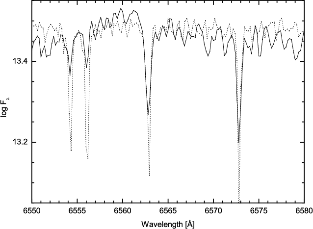
![]() log
log
![]() (Fig. 20). As expected, the molecular features are too weak and the H
(Fig. 20). As expected, the molecular features are too weak and the H![]() line can't be modeled in absorption without an emission core in this
series. It seems impossible to get a comparable fit for a model in
which only the abundances of
line can't be modeled in absorption without an emission core in this
series. It seems impossible to get a comparable fit for a model in
which only the abundances of ![]() elements relative to iron are enhanced.
elements relative to iron are enhanced.
|
Figure 18:
Temperature as a function of the optical depth at |
| Open with DEXTER | |
|
Figure 19:
Comparison of high resolution observations of Gl 1 (full line) and best model fit from Fig. 17. It is calculated with an additional cool chromosphere including convection with parameters
|
| Open with DEXTER | |
5 Discussion
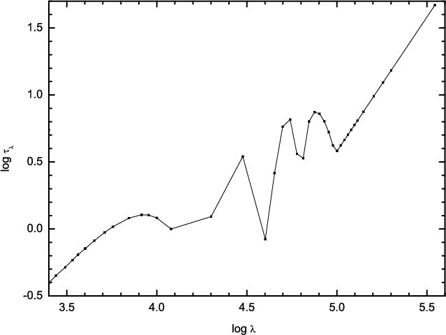
It had been the original plan (Wehrse et al. 1997) to detect - as a consequence of the strong increase of the H- absorption coefficient with wavelength - the chromosphere of M dwarfs in the IR range accessible to the ISO and Spitzer space crafts, and to use these observations to model empirically the temperature distributions in the very outer layers of these stars. This would allow the study of the outer radiative boundary condition needed in the construction of chromospheric and interior models.Unfortunately, a flux excess increasing to longer wavelengths is not seen for Gl 1 up to about 35 ![]() m. The reason for this can be seen from Fig. 21. In spite of a strong increase with wavelength,
m. The reason for this can be seen from Fig. 21. In spite of a strong increase with wavelength,
![]() (
(
![]() )
does yet not reach increase unity, i.e. we see essentially only the
layers around the temperature minimum! This is most probably the reason
for the flux decrease that is steeper than that of a black body
(Fig. 10).
With increasing wavelengths, layers of lower and lower temperature are
seen. Since we have not modelled the flux of Gl 1 consistently
from the UV to the IR (e.g. with respect to the inclusion of all
relevant lines),
we cannot give accurate total acoustic plus magnetic fluxes that are
dissipated in the chromosphere but our models indicate
an appreciable fraction (up to about 25%) of the total flux entering
the atmosphere must be of non-radiative nature.
If this is confirmed, these fluxes will have severe consequences for
the temperature stratification for layers below the
chromosphere also and must consistently be taken into account in future
modeling. This would imply that the effective temperature, the gravity,
and the chemical composition are not sufficient to determine the
atmospheres of M dwarf stars uniquely.
)
does yet not reach increase unity, i.e. we see essentially only the
layers around the temperature minimum! This is most probably the reason
for the flux decrease that is steeper than that of a black body
(Fig. 10).
With increasing wavelengths, layers of lower and lower temperature are
seen. Since we have not modelled the flux of Gl 1 consistently
from the UV to the IR (e.g. with respect to the inclusion of all
relevant lines),
we cannot give accurate total acoustic plus magnetic fluxes that are
dissipated in the chromosphere but our models indicate
an appreciable fraction (up to about 25%) of the total flux entering
the atmosphere must be of non-radiative nature.
If this is confirmed, these fluxes will have severe consequences for
the temperature stratification for layers below the
chromosphere also and must consistently be taken into account in future
modeling. This would imply that the effective temperature, the gravity,
and the chemical composition are not sufficient to determine the
atmospheres of M dwarf stars uniquely.
|
Figure 20:
Same as Fig. 16 but for parameters
|
| Open with DEXTER | |
|
Figure 21:
Essential run of the optical depth of the layer
|
| Open with DEXTER | |
The element abundances given in Sect. 4 have been determined
iteratively starting from solar values and seemed to give the best fits
to our spectra. In view of the complicated dependencies of the line
strengths and profiles on the details of the temperature stratification
and of the chemical composition (cf. Allard & Hauschildt 1995; see also Wehrse 1985, for an analogue discussion for M giants), we cannot, however, exclude
that a fit to the full spectrum may result in a somewhat different composition, e.g. in an enhanced abundance ratio of the ![]() elements to iron. A thorough quantitative error analysis on the basis
of well calibrated high dispersion spectra extending from the visible
to the infrared range is certainly an urgent need for cool dwarf stars
such as Gl 1.
elements to iron. A thorough quantitative error analysis on the basis
of well calibrated high dispersion spectra extending from the visible
to the infrared range is certainly an urgent need for cool dwarf stars
such as Gl 1.
In summary, we have analyzed high resolution optical and low
resolution infra-red spectra of the early M dwarf Gliese 1 in
order to study the temperature structure of the upper photospheric
layers. From the H![]() and adjacent metal line profiles it is found that there should be a temperature reversal at about
and adjacent metal line profiles it is found that there should be a temperature reversal at about
![]() and an outer temperature of
and an outer temperature of ![]() 4900 K. There are no indications of horizontal inhomogeneities or of chromospheric flux enhancements in the IR up to
4900 K. There are no indications of horizontal inhomogeneities or of chromospheric flux enhancements in the IR up to
![]() It was beyond the scope of this paper to perform a full and consistent
abundance analysis, the modeling of the metal lines requiered decreased
abundances for Ca, Fe and Ti.
It was beyond the scope of this paper to perform a full and consistent
abundance analysis, the modeling of the metal lines requiered decreased
abundances for Ca, Fe and Ti.
References
- Allard, F. 1990, Ph.D. Thesis, Ruprecht Karls Univ Heidelberg [Google Scholar]
- Allard, F., & Hauschildt, P. H. 1995, ApJ, 445, 433 [NASA ADS] [CrossRef] [Google Scholar]
- Bessell, M. S. 1990, A&AS., 83, 357 [Google Scholar]
- Bessell, M. S. 1991, AJ, 101, 662 [NASA ADS] [CrossRef] [Google Scholar]
- Brett, J. M., & Plez, B. 1993, Proc. Astron. Soc. Australia, 10, 250 [Google Scholar]
- Cincunegui, C., & Mauas, P. J. D. 2004, A&A, 414, 699 [Google Scholar]
- Cram, L. E., & Mullan, D. J. 1979, ApJ, 234, 579 [NASA ADS] [CrossRef] [EDP Sciences] [Google Scholar]
- Eggen, O. J. 1979, ApJ, 230, 786 [NASA ADS] [CrossRef] [Google Scholar]
- Evans, D. S. 1961, Royal Greenwich Observatory Bulletin, 48, 389 [NASA ADS] [Google Scholar]
- Gabriel, C., Acosta-Pulido, J., Heinrichsen, I., Morris, H., & Tai, W.-M. 1997, in Astronomical Data Analysis Software and Systems VI, ed. G. Hunt, & H. Payne, ASP, 125, 108 [Google Scholar]
- Giampapa, M. S. 1985, ApJ, 299, 781 [NASA ADS] [CrossRef] [Google Scholar]
- Gizis, J. E., Reid, I. N., & Hawley, S. L. 2002, AJ, 123, 3356 [NASA ADS] [CrossRef] [Google Scholar]
- Gliese, W. 1969, Veröffentlichungen des Astronomischen Rechen-Instituts Heidelberg, 22, 1 [Google Scholar]
- Golimowski, D. A., Leggett, S. K., Marley, M. S., et al. 2004, AJ, 127, 3516 [NASA ADS] [CrossRef] [Google Scholar]
- Gustafsson, B., Edvardsson, B., Eriksson, K., et al. 2003, in Stellar Atmosphere Modeling, ed. I. Hubeny, D. Mihalas, & K. Werner, ASP Conf. Ser., 288, 331 [Google Scholar]
- Gustafsson, B., Edvardsson, B., Eriksson, K., et al. 2008, A&A, 486, 951 [Google Scholar]
- Hauschildt, P. H., Allard, F., & Baron, E. 1999, ApJ, 512, 377 [NASA ADS] [CrossRef] [Google Scholar]
- Hawley, S. L., Gizis, J. E., & Reid, I. N. 1996, AJ, 112, 2799 [NASA ADS] [CrossRef] [Google Scholar]
- Hinkle, K., Wallace, L., Valenti, J., & Harmer, D. 2000, Visible and Near Infrared Atlas of the Arcturus Spectrum 3727-9300 Å, ed. K. Hinkle, L. Wallace, J. Valenti, D. Harmer [Google Scholar]
- Houck, J. R., Roellig, T. L., van Cleve, J., et al. 2004, ApJ, 154, 18 [Google Scholar]
- Houdebine, E. R., Doyle, J. G., & Koscielecki, M. 1995, A&A, 294, 773 [Google Scholar]
- Jefferies, J. T. 1968, Spectral line formation, ed. J. T. Jefferies [Google Scholar]
- Kurucz, R. L. 2005, Mem. Soc. Astron. Ital. Supp., 8, 189 [Google Scholar]
- Laureijs, R. J., Klaas, U., Richards, P. J., Schulz, B., & Abraham, P. 2003, The ISO Handbook, Vol. IV - PHT - The Imaging Photo-Polarimeter, ed. T.G. Mueller, J.A.D.L. Blommaert, & P. Garcia-Lario., ESA SP-1262 [Google Scholar]
- Leggett, S. K. 1992, ApJ, 82, 351 [Google Scholar]
- Leggett, S. K., & Hawkins, M. R. S. 1988, MNRAS, 234, 1065 [NASA ADS] [CrossRef] [Google Scholar]
- Lemke, D., Klaas, U., Abolins, J., et al. 1996, A&A, 315, L64 [Google Scholar]
- Mihalas, D. 1978, Stellar atmospheres, 2nd edition, ed. J. Hevelius [Google Scholar]
- Mould, J. R. 1975, A&A, 38, 283 [Google Scholar]
- Mould, J. R. 1976, A&A, 48, 443 [Google Scholar]
- Panagi, P. M., & Mathioudakis, M. 1993, A&AS, 100, 343 [Google Scholar]
- Plez, B. 1998, A&A, 337, 495 [Google Scholar]
- Reid, N., & Hawley, S. L., 2000, New light on dark stars: red dwarfs, low mass stars, brown dwarfs [Google Scholar]
- Robinson, R. D., Cram, L. E., & Giampapa, M. S. 1990, ApJS, 74, 891 [NASA ADS] [CrossRef] [Google Scholar]
- Short, C. I., & Doyle, J. G. 1997, A&A, 326, 287 [Google Scholar]
- Stauffer, J. R., & Hartmann, L. W. 1986, ApJS, 61, 531 [NASA ADS] [CrossRef] [Google Scholar]
- Wehrse, R. 1981, MNRAS, 195, 553 [NASA ADS] [Google Scholar]
- Wehrse, R. 1985, in Cool Stars with Excesses of Heavy Elements, Proceedings of the Strasbourg Observatory Colloquium, Universite de Strasbourg I, France, July 3-6, 1984 (Dordrecht: D. Reidel Publishing Co.) ed. M. Jaschek, & P. C. Keenan, Astrophysics and Space Science Library, 114, 293 [Google Scholar]
- Wehrse, R., Rosenau, P., Suvernev, A., Liebert, J., & Leinert, C. 1997, in The first ISO workshop on Analytical Spectroscopy, ed. A. M. Heras, K. Leech, N. R. Trams, & M. Perry, ESA SP, 419, 309 [Google Scholar]
All Tables
Table 1: Relevant parameters of Gl 1.
All Figures
|
|
Figure 1: ISOPHOT S (solid line) and IRS (dotted line) flux distributions for Gl 1. |
| Open with DEXTER | |
| In the text | |
|
|
Figure 2: The spectrum of Gl 1 in the range of 3910-4020 Å around the Ca II H and K lines with a resolution of 100 mÅ. Note the strong but very narrow emission in the cores of Ca II K (3933.7 Å) and Ca II H (3968.5 Å). |
| Open with DEXTER | |
| In the text | |
|
|
Figure 3: The spectrum of Gl 1 in the range of 4206-4324 Å around the Ca I line with a resolution of 100 mÅ. |
| Open with DEXTER | |
| In the text | |
|
|
Figure 4: The spectrum of Gl 1 in the range of 5860-6027 Å around the Na I D2 and D1 lines with a resolution of 200 mÅ. |
| Open with DEXTER | |
| In the text | |
|
|
Figure 5:
The spectrum of Gl 1 in the range of 6546-6730 Å around the H |
| Open with DEXTER | |
| In the text | |
|
|
Figure 6: The spectra of the stars Gl 1 (M1.5), Arcturus (K1.5) and the Sun (G2) from top to bottom in the range of 3910-4020 Å around the Ca II H and K lines. |
| Open with DEXTER | |
| In the text | |
|
|
Figure 7: The spectra of the stars Gl 1 (M1.5), Arcturus (K1.5) and the Sun (G2) from top to bottom in the range of 4206-4324 Å around the Ca I line. |
| Open with DEXTER | |
| In the text | |
|
|
Figure 8: The spectra of the stars Gl 1 (M1.5), Arcturus (K1.5) and the Sun (G2) from top to bottom in the range of 5860-6027 Å around the Na I D lines. |
| Open with DEXTER | |
| In the text | |
|
|
Figure 9:
The spectra of the stars Gl 1 (M1.5), Arcturus (K1.5) and the Sun
(G2) from top to bottom in the range of 6546-6730 Å around the H |
| Open with DEXTER | |
| In the text | |
|
|
Figure 10:
Flux distributions for Gl 1 as shown in Fig. 1 in
the range 3.5-35 |
| Open with DEXTER | |
| In the text | |
|
|
Figure 11: Distribution of the numbers of titanium oxide lines (Plez 1998) used in the modeling of the spectrum in the wavelength range 6550-6580 Å as a function of the gf-values of the lines. It is seen that there are essentially three peaks but the distributions are essentially continuous. |
| Open with DEXTER | |
| In the text | |
|
|
Figure 12:
Model series with gray temperature stratification for
|
| Open with DEXTER | |
| In the text | |
|
|
Figure 13:
Temperature as a function of the optical depth at |
| Open with DEXTER | |
| In the text | |
|
|
Figure 14:
Comparison of high resolution observations of Gl 1 (full line) and
synthetic spectra calculated with an additional cool chromosphere with
parameters
|
| Open with DEXTER | |
| In the text | |
|
|
Figure 15:
Same as Fig. 14 but for parameters
|
| Open with DEXTER | |
| In the text | |
|
|
Figure 16:
Synthetic spectra calculated with an additional cool chromosphere including convection with
|
| Open with DEXTER | |
| In the text | |
|
|
Figure 17:
Same as Fig. 16 but for parameters
|
| Open with DEXTER | |
| In the text | |
|
|
Figure 18:
Temperature as a function of the optical depth at |
| Open with DEXTER | |
| In the text | |
|
|
Figure 19:
Comparison of high resolution observations of Gl 1 (full line) and best model fit from Fig. 17. It is calculated with an additional cool chromosphere including convection with parameters
|
| Open with DEXTER | |
| In the text | |
|
|
Figure 20:
Same as Fig. 16 but for parameters
|
| Open with DEXTER | |
| In the text | |
|
|
Figure 21:
Essential run of the optical depth of the layer
|
| Open with DEXTER | |
| In the text | |
Copyright ESO 2010
Current usage metrics show cumulative count of Article Views (full-text article views including HTML views, PDF and ePub downloads, according to the available data) and Abstracts Views on Vision4Press platform.
Data correspond to usage on the plateform after 2015. The current usage metrics is available 48-96 hours after online publication and is updated daily on week days.
Initial download of the metrics may take a while.