Morphology of the local volume

M. Kerscher; A. Tikhonov

doi:10.1051/0004-6361/200912353

Home

All issues

Volume 509 (January 2010)

A&A, 509 (2010) A57

Full HTML

Free Access

Issue		A&A Volume 509, January 2010


Article Number		A57
Number of page(s)		9
Section		Cosmology (including clusters of galaxies)
DOI		https://doi.org/10.1051/0004-6361/200912353
Published online		19 January 2010

A&A 509, A57 (2010)

Morphology of the local volume

M. Kerscher¹ - A. Tikhonov²

1 - Mathematisches Institut, Ludwig-Maximilians-Universität, Theresienstrasse 39, 80333 München, Germany
2 - Saint-Petersburg State University, Russian Federation

Received 20 April 2009 / Accepted 21 October 2009

Abstract
To study the global morphology of the galaxy distribution in our local neighbourhood we calculate the Minkowski functionals for a sequence of volume limited samples within a sphere of 8 Mpc centred on our galaxy. The well known strong clustering of the galaxies and the dominance of voids and coherent structures on larger scales is clearly visible in the Minkowski functionals. The morphology of the galaxy distribution changes with the limiting absolute magnitude. The samples, encompassing the more luminous galaxies, show emptier voids and more pronounced coherent structures. Indeed there is a prominent peak in the luminosity function of isolated galaxies for $M_B\approx-14$ , which at least partly explains these morphological changes. We compare our date with halo samples from a $\Lambda$ CDM simulation. Special care was taken to reproduce the observed local neighbourhood as well as the observed luminosity function in these mock samples. All in all the mock samples render the global morphology of the galaxy distribution quite well. However, the detailed morphological analysis reveals that real galaxies cluster stronger, the observed voids are emptier and the structures are more pronounced compared to the mock samples from the $\Lambda$ CDM simulation.

Key words: galaxy: formation - large-scale structure of Universe

1 Introduction

We study the global morphology of the galaxy distribution in the local volume using Minkowski functionals and compare the geometry and topology of the galaxy distribution to halo samples from a $\Lambda$ CDM-simulation. Only in our local neighbourhood are we able to observe objects down to very low absolute luminosities, and only there will we be able to construct an almost complete galaxy sample. Karachentsev et al. (2004) presented the essential version of such a catalogue of neighbouring galaxies. They outlined the main structural elements of the local volume: the local sheet (part of the local supercluster), the groups containing about 2/3 of the total local volume population and the local (Tully) void (and some other voids). Tikhonov & Karachentsev (2006) and Tikhonov & Klypin (2009) analysed these voids and the galaxy distribution within. To study the global morphology of the galaxy distribution we use the same data - an updated catalogue of neighbouring galaxies (Karachentsev, private communication).

Cold dark matter simulations together with a cosmological constant ( $\Lambda$ CDM-simulations) are considered to match the distribution of M^*-like galaxies quite well. However, there are problems on small scales with the abundance of small mass aggregations. The $\Lambda$ CDM model predicts thousands of dwarf dark matter halos in the local group (Moore et al. 1999; Madau et al. 2008; Klypin et al. 1999a), while only $\sim$ 50 are observed. Recently Tikhonov & Klypin (2009) found in $\Lambda$ CDM-simulations a severe overabundance (a factor of 10) of halos in the voids compared to the observed number of galaxies in nearby voids. The overabundance of halos on small mass scales as well as in the voids is certainly a problem for the $\Lambda$ CDM-model. In the present study, we investigate the spatial distribution of halos from a $\Lambda$ CDM simulation compared to the galaxies observed in the local volume. For the comparison with halo samples, we use the procedure from Tikhonov & Klypin (2009) to map the circular velocities of the dark matter halos to luminosities. This allows the construction of mock galaxy samples with the same number of objects and the same luminosity function as observed in the galaxy sample from the local volume. Hence, we assume that the $\Lambda$ CDM overabundance can either be solved by the detection of new (very) low surface brightness galaxies, or by mechanisms suppressing the galaxy formation in small dark halos (see Tikhonov & Klypin 2009, for a discussion and references). Our focus is on the global morphology of the galaxy distribution compared to the halo distribution.

1.1 The galaxy sample

Over the past few years searches for galaxies with distances less than 10 Mpc have been undertaken using numerous observational data including searches for low surface brightness galaxies, blind HI surveys, and NIR and HI observations of galaxies in the zone of avoidance (Karachentsev et al. 2007,2004). The sample contains about 550 galaxies (see Fig. 1),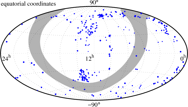

$\begin{figure} \par\resizebox{8.5cm}{!}{\includegraphics{12353f1.eps}} \end{figure}$	Figure 1: The distribution of the galaxies in the local volume on the sky.
Open with DEXTER

the distances to the galaxies are measured independent of the redshift, mostly with tip of the red giant brunch stars, cepheids, the Tully-Fisher relation, and some other secondary distance indicators. The galaxies in the local volume sample map the ``real'' 3D distribution. The absence of the ``fingers of God''-effect simplifies the morphological analysis of the local volume. The distances have been measured with an accuracy of 8-10% for most of the galaxies (Karachentsev et al. 2004). According to Karachentsev (2007, private communication) this sample is nearly volume-limited within an 8 Mpc radius from our galaxy and is reasonably complete for galaxies with an absolute magnitude of $M_B\le -12$ . Some density gradients visible in the local volume sample are not necessarily caused by an incompleteness. They can be explained more naturally with structures in the local volume. The majority of groups resides in a thin layer with a distance of <0.3 Mpc from the supergalactic plane. The filaments of the local supercluster fall mainly in the supergalactic plane, causing an excess of galaxies in this region compared to the outer regions which are perpendicular to the supergalactic plane. The overall completeness of this sample is discussed in Tikhonov & Klypin (2009). They concluded that a significant incompleteness of the sample is improbable. There still exists the possibility that the observational sample is incomplete, missing very low surface brightness galaxies free from gas, beyond the sensitivity of modern ground-based telescopes. The limiting magnitudes and the number of galaxies in the subsamples considered are summarised in Table 1.

Table 1: The galaxy samples considered.

1.2 Minkowski functionals

$\begin{figure} \par\includegraphics[width=9cm,clip]{12353f2.eps} \vspace*{-4mm} \end{figure}$	Figure 2: Galaxies from the local volume decorated with balls of varying radii.
Open with DEXTER

The genus of an isodensity surface is a well known method to describe the topology of cosmological density fields (Gott III et al. 1987). Minkowski functionals provide a unifying framework for the topology and the geometrical quantities like volume, surface area, and integrated mean curvature. They have been developed for the morphological characterisation of the large scale distribution of galaxies and galaxy clusters by Mecke et al. (1994) and have successfully been used in cosmology (Kerscher 2000; Kerscher et al. 1997), porous and disordered media, dewetting phenomena, fluid and magneto hydrodynamics (see Mecke 2000, for a review).

In order to quantify the spatial distribution of the galaxies we decorate the galaxies with balls of varying radii (see Fig. 2). Consider the union set $A_r=\bigcup_{i=0}^N B_r({x}_i)$ of balls of a radius r around the N galaxies at the positions x_i, $i=1,2,\dots N$ , thereby creating connections between neighbouring balls. The global morphology of the union set of these balls changes with the radius r, which is employed as a diagnostic parameter. It seems sensible to request that global geometrical and topological valuations of e.g. A_r are additive, invariant under rotations and translations, and are continuous, at least for convex bodies. With these prerequisites Hadwiger (1957) could show that in three dimensions the four Minkowski functionals $M_{\mu}(A_r)$ , $\mu = 0,1,2,3$ , give a complete morphological characterisation of the body A_r. The Minkowski functional M₀(A_r) is simply its volume, M₁(A_r)is an eight of its surface area, M₂(A_r) is its mean curvature divided by $2\pi^2$ , and M₃(A_r) is its Euler characteristics multiplied by $\frac{3}{4\pi}$ . Volume and surface area are well known quantities. The integral mean curvature and the Euler characteristic are defined as surface integrals over the mean and the Gaussian curvature respectively. This definition is only applicable for bodies with smooth boundaries. In our case we have additional contributions from the intersection lines and intersection points of the balls. Mecke et al. (1994) discuss the extension for a union set of convex bodies.

One may express Minkowski functionals in terms of n-point correlation functions, similar to a perturbative expansion. But the strength of an analysis with Minkowski functions is the direct quantification of the morphology. The additivity of the local contributions to the Minkowski functionals ensures the robustness of the Minkowski functionals even for small point sets (Mecke et al. 1994). In an analysis with Minkowski funtionals, using up to 385 galaxy clusters from the REFLEX sample, Kerscher et al. (2001) were able to clearly distinguish the distribution of observed galaxy clusters from a Gaussian point distribution. As can bee seen from the Table 1 we are confronted with samples with a similar (small) number of points. Closely related to our analysis is the investigation of the void sizes, as performed by Tikhonov & Klypin (2009) for the same catalogue of nearby galaxies. Indeed the void probability distribution function is equal to one minus the volume density, the first Minkowski functional. Hence our analysis complements these investigation by additionally using the other three Minkowski functionals, to quantify the geometry, shape and topology of the galaxy sample.

2 Morphology of the local volume

$\begin{figure} \par\includegraphics[width=11.5cm,clip]{12353f3.eps} \end{figure}$	Figure 3: The volume densities $m_\mu (A_r)$ of the Minkowski functionals determined from the galaxy samples `lv8m12` (black, solid), `lv8m14` (red, dotted), `lv8m15` (blue, dashed), `lv8m16` (green, dashed dotted) For reference the $m_\mu (A_r)$ of a Poisson process with the same number density as `lv8m12` are shown (one- $\sigma$ area, thin black lines).
Open with DEXTER

The galaxy and halo samples considered are only complete within a radius of 8 Mpc. We use the boundary corrections as discussed in Appendix A to calculate the volume densities of the Minkowski functionals in an unbiased way. In Appendix B we show how the Minkowski functionals describe the morphological features and briefly discuss some stochastic models.

In Fig. 3 we show the volume densities $m_\mu (A_r)$ of the Minkowski functionals for a series of volume limited samples from the local galaxy distribution. For reference the functionals of randomly distributed points (Poisson process) are shown.

Compared to randomly distributed points, the volume density m₀(A_r)increase is considerably delayed for all of the galaxy samples. The empty space in between the strongly clustering galaxies fills up later than for the purely random distribution.

The balls on the clustering galaxies already overlap for small radii, causing a slow rise and a reduced maximum of the surface density $m_1(A_r)\times8$ compared to Poisson distributed points. For large radii the surface density of the galaxies is above the values for randomly distributed points. The galaxies cluster on low dimensional structures, and consequently the balls have more room to grow. In Sect. 2.1 we will comment on the excess surface density in the samples with an absolute magnitude $M_B\le-15$ , as its is visible for large radii.

Again, due to the clustering, the density of the integral mean curvature $m_2(A_r)2\pi^2>0$ increases slower and the maximum is reduced in comparison to a Poisson process. In a Poisson process we get completely enclosed voids leading to the strong negative signal. However, only a week negative signal is seen from the galaxy samples. The concave structures are less prominent, as is to be expected for clustering on planar (super galactic plane) or even filamentary structures.

For the radius r=0 the density of the Euler characteristic $m_3(A_0)\frac{4\pi}{3}$ equals the number density of the galaxies in the sample. Hence the difference at r=0 is only a reflection of the different sampling. With an increasing radius more and more balls overlap and the Euler characteristic decreases. Then tunnels through the structure are forming, giving a negative contribution to m₃(A_r). In the galaxy distribution only a small positive value for m₃(A_r)can be observed, strengthening the previous observation that the voids are not completely enclosed.

2.1 Morphology changing with the absolute magnitude

We get the impression already from Fig. 3 that the morphology of the galaxy distribution changes significantly if we include galaxies with absolute magnitudes $M_B\le-15$ in our analysis. However, we have to be more careful. Minkowski functionals calculated from points decorated with balls do depend on the number density of the point distribution. One can derive an explicit expression in terms of high order correlation functions quantifying this non-trivial dependence on the number density (see e.g. Mecke 2000). To compare the galaxy distributions with different limiting magnitudes we generate samples with the same number of points. We randomly subsample the galaxy samples lv8m12 and lv8m14 to the same number density as in the sample lv8m15. This allows us to compare the volume densities $m_\mu (A_r)$ for the galaxy sample with $M_B\le -12$ , $M_B\le -14$ and $M_B\le-15$ in Fig. 4. The Minkowski functionals of the samples with $M_B\le -12$ and $M_B\le -14$ agree within the error bars. Also the volume density and the Euler characteristic mostly agree between all the samples, whereas the sample with $M_B\le-15$ shows an increased surface density m₁(A_r) for radii from 2.2 to 3.2 Mpc. The voids become significantly more emptier going from a limiting magnitude $M_B\le -14$ to $M_B\le-15$ . For the density of the integral mean curvature m₂(A_r) we see that the negative contributions occur only for larger radii in the $M_B\le-15$ sample. These emptier voids are surrounded by concave structures at larger radii.

$\begin{figure} \par\includegraphics[width=11.5cm,clip]{12353f4.eps} \end{figure}$	Figure 4: Volume densities $m_\mu (A_r)$ of the Minkowski functionals determined from the galaxy samples `lv8m15` (blue solid) compared to the subsampled galaxy samples `lv8m14` (red dashed) and `lv8m12` (black, one- $\sigma$ error from randomly subsampling).
Open with DEXTER

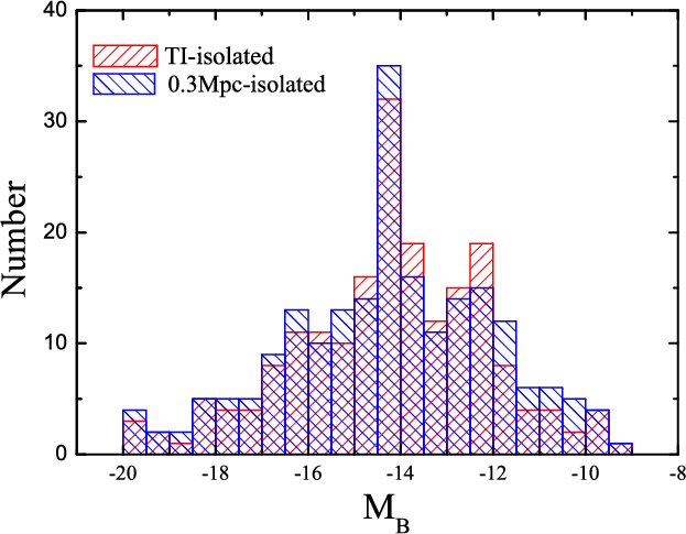
This behaviour can be explained by looking at the luminosity function of isolated galaxies in the samples. Figure 5 shows the number of isolated galaxies in the local volume versus the absolute B magnitude.

$\begin{figure} \par\resizebox{8.8cm}{!}{\includegraphics{12353f5.eps}} \end{figure}$	Figure 5: The number of isolated galaxies shown for bins of absolute magnitude M_B. Either a geometrical neighbourhood criterion (0.3 Mpc-isolated) or a dynamical criterion based on the tidal index (TI) are used to determine isolated galaxies.
Open with DEXTER

We use two selection criteria for isolated galaxies: first a geometrical one - an isolated galaxy may not have any neighbour within a distance of 0.3 Mpc, which is close to the virial radius of an M^* galaxy. As a second criterion we use the tidal index (TI) of Karachentsev et al. (2004), comparing a local dynamical timescale of the galaxy to the Hubble time. We consider galaxies with a tidal index less than zero as isolated. As can be seen from Fig. 5 the abundances of galaxies selected by either geometrical or physical criteria match. In both cases the same prominent feature shows up, a peak in the number of isolated galaxies with an absolute Magnitude $M_B\sim-14$ . This peak explains that mainly isolated galaxies are lost in going from the sample lv8m14 with $M_B\le -14$ to the more luminous sample lv8m15 with $M_B\le-15$ . It is reasonable to assume that isolated galaxies predominantly reside in voids. Then the voids are emptier in lv8m15, which is exactly what we observe with the Minkowski functionals.

2.2 Error estimates

The position of a galaxy on the sky is known with a high accuracy. However, the radial distance is estimated with some distance indicator. To quantify the influence of the distance error on our estimates of the Minkowski functionals we randomise the radial distance r using a Gaussian probability law with mean r and standard deviation 0.1 r. We observe that the Minkowski functionals of the randomised samples closely follow the functionals of the galaxy sample, well within the error bars. We compare this measurement error to the statistical error of randomly distributed points with the same number density. This Poisson error is approximately twice as large as the measurement error obtained from randomising the distances. Also the error from the subsampling (sometimes called Jackknife error, see Fig. 4) has approximately the same amplitude as the Poisson error.

3 Comparison with mock samples

The local volume is certainly not a fair sample of the Universe. However, only within our local neighbourhood are we able to probe the galaxy distribution down to very low absolute luminosity. In the local volume we have prominent structural elements like the Tully void and the supergalactic plane. The extraction of mock samples requires a careful selection of the position in the simulation box to find comparable features. Moreover the simulation has to be performed in a box large enough to allow those structures to form and, on the other side, with enough resolution on small scales to resolve the low mass halos.

3.1 Simulation

We use N-body simulation provided by A. Klypin done with the Adaptive Refinement Tree code (Kravtsov et al. 1997). The simulation was performed in a box with side lengths 160 h^-1 Mpc for a spatially flat cosmological $\Lambda$ CDM model, which is compatible with the 3rd year WMAP data (Spergel et al. 2007) with the parameters h=0.73, $\Omega_{\rm m}=0.24$ , $\Omega_\textrm{\tiny bar}=0.042$ , $\Omega_{\Lambda}=0.76$ , and the normalisation $\sigma_8 = 0.75$ . In this simulation the total number of particles is 1024³, the mass of a particle is $3.18\times 10^8~h^{-1}~M_{\odot}$ , the spatial resolution is 1.2 h^-1 kpc, and the circular velocity of the smallest resolved halo is 27 km s^-1. We re-scaled all data (coordinates and masses of halos) to real units assuming H₀=72 km s^-1 Mpc^-1, which is close to the value reported from the WMAP analysis. Halos are extracted using the bound density maximum halo finder (Klypin et al. 1999b), which detects bound halos with their subhalos and calculates several physical and geometrical parameters of these (sub)halos. We use the maximum circular velocity $V_{\rm c}$ to rank order the halos. The maximum circular velocity $V_{\rm c}$ can be determined more dependantly from the simulations and is easier to relate to observations compared with the virial mass. We have a monotone relation between mass and circular velocity $V_{\rm c}$ . For reference, halos with V_c=50 km s^-1 have a virial mass of approx. $10^{10}~M_{\odot}$ and halos with $V_{\rm c}=20$ km s^-1 have a virial mass of approx. $10^{9}~M_{\odot}$ .

3.2 Selection of a neighbourhood comparable to the local volume

The reasonably big volume of the simulation box allows us to select mock samples that mimic the local volume features more closely. As in Tikhonov & Klypin (2009) we use several criteria to select spheres with a radius of 8 Mpc from the simulation box:

1.: no halos with a mass of > $2\times 10^{13}~M_{\odot}$ reside inside the 8 Mpc sphere;
2.: the sphere must be centred on a halo with $1.5\times 10^{12}~M_{\odot} < \textit{mass} < 3\times 10^{12}~M_{\odot}$ km s^-1 (the local group analog);
3.: the number density of halos with $V_{\rm c}>100$ km s^-1 inside the 8 Mpc sphere exceeds the mean value in the whole box by a factor ranging from 1.5 to 1.7;
4.: the number density of halos with $V_{\rm c}>100$ km s^-1 found inside a 4.5 Mpc sphere exceeds the mean value in the whole box by a factor greater than 4;
5.: there is no halo more massive than $5.0\times 10^{11}~M_{\odot}$ with a distance in the range from 1 to 3 Mpc;
6.: the central halos of other mock samples are more distant than 16 Mpc. There is no overlap between the samples.

As discussed in Tikhonov & Klypin (2009), samples selected by the above criteria may be considered as close geometrical and physical cousins of the real local volume. We could select five such samples from the simulation box. Visual inspection shows that our mock samples look quite similar to the local volume galaxy sample.

3.3 Mapping between luminosity and circular velocity of the halos

When assigning luminosities to dark matter halos we follow the prescription of Conroy et al. (2006): first we build an ordered list of all the galaxies in the observed local volume sample ranked by their luminosity. Then we rank-order the halos in our local volume candidate-samples by their circular velocity. Now the luminosity of the brightest galaxy is assigned to the halo with the largest circular velocity. Then the luminosity of the second brightest galaxy is assigned to the second biggest halo and so on. This procedure preserves the galaxy luminosity function, and our mock samples have the same number density as the observed galaxy sample (see Table. 1). By construction we have a monotonic relation between $V_{\rm c}$ and M_B. Conroy et al. (2006) showed that this prescription reproduces also the clustering properties of the more massive galaxies in SDSS samples. Nonetheless this mapping is not perfect. Only halos with $V_{\rm c}>30$ km s^-1 are left within the mock samples, whereas in the observed sample galaxies those with $M_B\approx -12$ may have a significantly lower circular velocity (Tikhonov & Klypin 2009). However, if we would assign higher luminosities also to halos with small circular velocities, we would end up with too many halos.

3.4 Morphological comparison

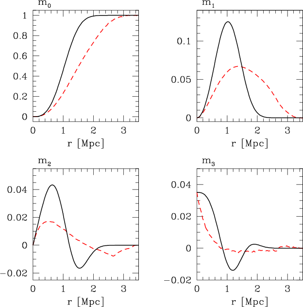
In Figs. 6-8 we compare the morphology of the galaxy distribution to the morphology of the corresponding halo samples from the $\Lambda$ CDM simulation. We show the average and the one- $\sigma$ range for the volume densities of the Minkowski functionals estimated from the five mock samples.

The surface area, the integral mean curvature and the Euler characteristic from the $M_B\le -14$ galaxy sample are well reproduced by the corresponding mock samples as seen in Fig. 7. Only the volume density m₀ is slightly reduced on large scales, indicating emptier voids.

This changes if we compare the mock samples with the galaxy samples including less luminous galaxies with a limiting absolute magnitude $M_B\le -12$ (see Fig. 6). The stronger clustering of the galaxies is visible in the steeper decrease of the Euler characteristic m₃(A_r) for small r and the reduced maximum of the integral mean curvature m₂(A_r). The well known fact that the voids are emptier in the real galaxy distribution can be seen from the reduced m₀(A_r) for large r.

The more luminous halo samples with $M_B\le -16$ also show some morphological discrepancies compared to the corresponding galaxy sample (Fig. 8). m₀(A_r) is reduced for large radii, and we conclude that the voids are emptier in the real galaxy distribution. Another phenomenon shown for the larger radii is that the halo samples do not show the pronounced coherent structures visible in the galaxy distribution, as can be seen from the increased surface density m₁(A_r) of the galaxy samples as compared to the halo samples.

$\begin{figure} \par\includegraphics[width=11cm,clip]{12353f6.eps} \end{figure}$	Figure 6: Volume densities $m_\mu (A_r)$ of the Minkowski functionals determined from the galaxy samples with $M_B\le -12$ (short dashed red lines) compared to averages over the corresponding halo samples (shaded $1\sigma$ area).
Open with DEXTER

$\begin{figure} \par\includegraphics[width=11cm,clip]{12353f7.eps} \end{figure}$	Figure 7: Volume densities $m_\mu (A_r)$ of the Minkowski functionals determined from the galaxy samples with $M_B\le -14$ (short dashed red lines) compared to averages over the corresponding halo samples (shaded $1\sigma$ area).
Open with DEXTER

$\begin{figure} \par\includegraphics[width=11cm,clip]{12353f8.eps} \vspace*{-2mm} \end{figure}$	Figure 8: Volume densities $m_\mu (A_r)$ of the Minkowski functionals determined from the galaxy samples with $M_B\le -16$ (short dashed red lines) compared to averages over the corresponding halo samples (shaded $1\sigma$ area).
Open with DEXTER

As we have seen in Sect. 2.1, the morphology of the observed galaxy distribution is depending on the limiting magnitude. To investigate this behaviour in the mock halo samples we proceed in the same way as in Sect. 2.1 and randomly subsample the halo samples corresponding to $M_B\le -12$ and $M_B\le -14$ to the same number density as seen in the $M_B\le-15$ sample. The morphology of the halo distribution only shows a week trend, still within the error bars, if we consistently select galaxies with higher circular velocities. Hence, the physical mechanisms leading to these emptier voids for $M_B\le-15$ in the observed galaxy distribution (cf. Fig. 4) are not captured by the $\Lambda$ CDM model, and/or the mapping from the circular velocity to the luminosity is more complicated at the faint end of the luminosity function.

4 Summary and discussion

To quantify the global morphology of the nearby galaxy distribution we calculated Minkowski functionals from a series of volume-limited samples extracted from the local volume galaxy catalogue (an updated version of the Catalogue of Nearby Galaxies from Karachentsev et al. 2004). These samples are nearly complete for $M_B\le -12$ within a distance of 8 Mpc from our galaxy. The strong clustering dominates the morphology of the galaxy samples on small scales. On larger scales the empty voids and coherent structures show up in the Minkowski functionals. It seems quite obvious to attribute these morphological features to the Tully void, covering approximately a quarter of the sample, and the supergalactic plane. By extracting a series of volume-limited samples with increasing luminosity we encountered a clear change in the global morphology of the galaxy distribution. Going from a sample with $M_B\le -14$ to the more luminous sample with $M_B\le-15$ the voids become significantly emptier. Indeed we saw a prominent peak in the luminosity function of isolated galaxies with $M_B\approx-14$ . We verified from the catalogue that all these galaxies are dwarf irregulars with significant relative star formation rates and hydrogen mass. Excluding these galaxies from a sample makes voids significantly emptier. It will be interesting to check if these galaxies form a unique population and to which extend selection effects or true physical effects cause the peak in the luminosity function. We mad sure that the errors in the distance indicators do not influence our results.

In the second part of the Paper we compared the morphology of the galaxy distribution to mock samples from a $\Lambda$ CDM simulation. The position of our mock samples inside the simulation box was chosen to mimic the main features of our real galactic neighbourhood, and the luminosities have been assigned to the halos in such a way that the observational number density and luminosity function are preserved. The overall picture, with clustering on small scales, large voids and coherent structures on large scales can also be seen in the morphology of the mock samples. This fundamental agreement allows us to look at the morphology in more detail. In spite of the careful selection of the mock samples we still see morphological differences between mock and galaxy samples. The galaxies cluster stronger and the observed voids are emptier than in the mock samples. This observation is going beyond the well known overabundance of halos in $\Lambda$ CDM models. By construction we have the same number of objects in the mock sample as in the galaxy sample, and we enforce the same luminosity function. Hence we see differences in the geometry and topology of the spatial distributions. Clearly, five mock samples do not allow any elaborate statistical tests (see e.g. Besag & Diggle 1977), but we may calculate a rough estimate of the fluctuations in the Minkowski functionals. These fluctuations are on the same order as those observed for a Poisson process. Therefore we claim to see differences in the morphology only if the Minkowski functionals are consistently outside the one- $\sigma$ range.

Certainly, our procedure of assigning luminosities to halos is oversimplified. Especially for low luminosities the mapping between the halo circular velocity and luminosity may not be straightforward. With our mapping only halos with a circular velocity of $V_{\rm c}>30$ km s^-1 are left in the mock samples. This agrees with theoretical predictions for the least massive halo that can host a galaxy (see e.g. Hoeft et al. 2006; Loeb 2008). However, in reality one observes galaxies with M_B in the range from -12 to -13 with significantly lower rotational velocities (Tikhonov & Klypin 2009). If we assign higher luminosities to halos with small circular velocities $V_{\rm c}$ we either end up with too many mock galaxies, or we would have to drop some halos with high $V_{\rm c}$ to keep the number of mock galaxies equal to the observed number. Such a procedure would break the monotonic relation between $V_{\rm c}$ and M_B. To generate larger emptier voids in the mock samples, one would have to additionally include halos with small $V_{\rm c}$ residing in the vicinity of filaments and sheets, and drop halos mainly residing in voids. Also halos in voids with a small $V_{\rm c}$ would have to remain dim. A more intricate environment-dependent modelling of the luminosities for the mock halos seems necessary, especially if we also want to understand the dependence of the global morphology on the absolute magnitude cut in our galaxy samples.

Another factor explaining the morphological discrepancies might be that all the five mock samples we could extract do not hold a void which is comparable in its size to the local (Tully) void. This allows two lines of arguments, either one blames the observations or the simulation. Looking at Fig. 1 we see that the zone of avoidance (our galaxy) cuts right through the Tully void. However, several targeted and blind searches of the zone of avoidance have been performed. It is unlikely that we actually miss enough galaxies to cut the void into halves (Karachentsev et al. 2004). On the other hand the simulation was conducted in a box with a side length of 160 h^-1 Mpc. This size is considered to be reasonably large, since we are only interested in mock samples within a sphere of 8 Mpc radius. It remains an open question whether a $\Lambda$ CDM simulation in a larger box could provide us with mock samples with big enough voids, especially when we consider the halo distribution at the low mass end of the mass function.

Acknowledgements

We thank I.D. Karachentsev for providing us with an updated list of his catalogue of neighbouring galaxies and A. Klypin for providing results of computer simulations that were conducted on the Columbia supercomputer at the NASA Advanced Supercomputing Division. Anton Tikhonov acknowledges support from the Deutsche Forschungsgemeinschaft (DFG grant: GO 563/17-1), and the ASTROSIM network of the European Science Foundation (ESF) and wishes to thank the Astrophysical Institute Potsdam for their hospitality.

Appendix A: Calculating Minkowski functionals

The code used for the calculations of the Minkowski functionals is an updated version of the code developed by Kerscher et al. (1997), based on the methods outlined in Mecke et al. (1994). The code is made available to the general public via http://www.math.lmu.de kerscher/software/

Below we present the boundary corrections used by Schmalzing et al. (1996). All galaxies in our samples are within a sphere of a radius R=8 Mpc around our galaxy, and the same applies to the halo samples. Let D_Rbe this spherical window containing N galaxies. $A_r=\bigcup_{i=1}^NB_r(i)$ is the union of balls B_r(i) of a radius r centred on the ith galaxy, respectively.

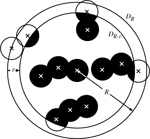
$\begin{figure} \par\resizebox{7.5cm}{!}{\includegraphics{12353f9.eps}} \end{figure}$	Figure A.1: A two-dimensional sketch illustrating the geometry of the boundary corrections used. R=8 Mpc is the radius of the sphere D_R centred on our galaxy enclosing the local sample. r is the radius of the individual balls centred on each galaxy, and the black area is the set $A_r\cap D_{R-r}$ .
Open with DEXTER

Considering only A_r we miss contributions from galaxies outside D_R, i.e. from galaxies not included in our sample. A well-defined way is offered by looking at the intersection $A_r\cap D_{R-r}$ (Mecke & Wagner 1991). Using the shrunken window D_R-r we make sure that all possible contributions are taken into account, as illustrated in Fig. A.1. In order to measure the boundary contributions we have to calculate the Minkowski functionals $M_\mu(A_r\cap{D_{R-r}})$ of the intersection of the union of all balls with the window, and the Minkowski functionals $M_\mu(D_{R-r})$ of the window D_R-r itself,

Now imagine the union set $\widetilde A_r$ of balls on all galaxies in a very large (but still finite) patch of the Universe, with $A_r\subset\widetilde A_r$ . Integrating over all movements (translations and rotations) of the window within this large patch of the universe we obtain the spatial average

$\begin{displaymath}\left\langle M_\mu\left(\widetilde A_r \cap D_{R-r}\right) \r... ...{G}} M_\mu\left(\widetilde A_r \cap gD_{R-r}\right) {\rm d} g. \end{displaymath}$

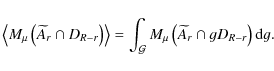
(A.1)

Here gD_R-r is a translation and/or rotation of the shrunken window, $\mathcal{G}$ is the group of motions, and ${\rm d}g$ the suitably normalised Haar-measure on this group. The integral over motions can be expressed as a sum using the principal kinematical formula (Hadwiger 1957)

$\begin{displaymath} \int_\mathcal{G} M_\mu\left(\widetilde A_r\cap gD_{R-r}\righ... ...nd{array}\!\right) M_\nu(\widetilde A_r) M_{\mu-\nu}(D_{R-r}). \end{displaymath}$

(A.2)

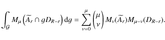
For a homogeneous and isotropic galaxy distribution the spatial average coincides with the expectation over different realizations, and $M_\mu(A_r\cap{D_{R-r}})$ is already an unbiased estimate of $\left\langle M_\mu\left(\widetilde A_r \cap D_{R-r}\right) \right\rangle$ . This observation together with Eq. (A.2) allows us to remove the boundary contribution of the window. For the volume density this is almost trivial:

$\begin{displaymath}m_0(A_r) = \frac{M_{0}(A_r\cap D_{R-r})}{M_0(D_{R-r})}\cdot \end{displaymath}$

(A.3)

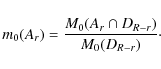
For all the Minkowski functionals estimates for the volume densities can be obtained by applying the following recursive formula (Fava & Santaló 1978):

$\begin{displaymath} m_\mu(A_r) = \frac{M_\mu(A_r \cap D_{R-r})}{M_0(D_{R-r})} - ... ...ht) m_\nu(A_r) \frac{M_{\mu-\nu}(D_{R-r})}{M_0(D_{R-r})}\cdot \end{displaymath}$

(A.4)

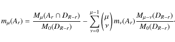
This linear transformation of the observed $M_\mu(A_r\cap{D_{R-r}})$ facilitates the direct comparison with the volume densities $m_\mu\left(\widetilde A_r\right)$ calculated from Point process models, namely the Poisson process.

Appendix B: Morphology with Minkowski functionals

Below we give a qualitative discussion of the Minkowski functionals for a Poisson process decorated with balls of radius r and relate them to the observed morphological features. The Minkowski functionals of randomly distributed points (a Poisson process) are shown in Fig. B.1.

$\begin{figure} \par\resizebox{8.8cm}{!}{\includegraphics{12353f10.eps}} \end{figure}$	Figure B.1: The volume densities $m_\mu (A_r)$ of the Minkowski functionals determined from a Poisson process (solid black lines) and points randomly distributed on random line segments (dashed red lines). Both models have the same number of points and the same sample geometry as the galaxies in `lv8m12`.
Open with DEXTER

With an increasing radius r the volume is filled until reaching complete coverage where the volume density m₀(A_r) reaches unity. The surface density $m_1(A_r)\times8$ increases with the radius r, reaches a maximum, and finally approaches zero when the volume is filled up and no surface area is left. For small radii the balls grow outwards and the positive density of the integral mean curvature $m_2(A_r)2\pi^2>0$ is a reflection of the mainly convex structure of the union set of balls. The volume starts to fill and the integral mean curvature reaches a maximum. For even larger radii we get negative contributions to the density of integral mean curvature stemming from concave structures - the balls are growing inward into the voids. Finally m₂(A_r) approaches zero when no surface area is left. For the radius r=0 each ball (point) gives a contribution of one to the Euler characteristics and the density of the Euler characteristic $m_3(A_0)\frac{4\pi}{3}$ equals the number density of the sample. With increasing radius more an more balls overlap and the Euler characteristic decreases. Then tunnels through the structure are forming, giving a negative contributions to m₃(A_r). As a clear signal of completely enclosed voids in the Poisson process, m₃(A_r) shows a second positive maximum.

Beyond the completely random model one may consider geometrically inspired models, e.g. points randomly distributed on randomly placed line segments. Minkowski functionals for such a low dimensional Poisson processes embedded in three dimensions are discussed by Schmalzing & Diaferio (2000). As anexample we show the Minkowski functionals for a model using in the mean 2.1 points, randomly distributed on randomly placed line segments with a length of 8 Mpc. As can be seen from Fig. B.1 some of the morphological features of the galaxy distribution discussed in Sect. 2 can be reproduced. Specifically the stronger clustering and the suppression of completely enclosed voids is clearly seen in the Minkowski functionals. The choice of these parameters does not seem realistic. Choosing more points per line segment or using shorter segments leads to largely different values for the Minkowski functionals. Indeed Schmalzing & Diaferio (2000) have shown that only with (random) mixtures of similar Poisson models for filament-, sheet- and field-galaxies one can reproduce the small scale morphology of the galaxy distribution. As can be seen from their Fig. B1 these mixture models are not appropriate on larger scales. This is expected, since randomly placed geometrical objects will not be able to model coherent large scale features. Other models are based on the hierarchy of correlation functions. The explicit incorporation of higher moments for the construction of point process models is discussed in Kerscher (2001). At least for the lowest order models the Minkowski functionals can be given explicitly (Kerscher et al. 2001). Models motivated from statistical physics and spatial statistics are discussed by Mecke (2000) and Mecke & Stoyan (2005).

References

Besag, J., & Diggle, P. J. 1977, Appl. Statist., 26, 327 [CrossRef] [Google Scholar]
Conroy, C., Wechsler, R., & Kravtsov, A. 2006, ApJ, 647, 201 [NASA ADS] [CrossRef] [Google Scholar]
Fava, N. A., & Santaló, L. A. 1978, J. Appl. Prob., 15, 494 [CrossRef] [Google Scholar]
Gott III, J. R., Weinberg, D. H., & Melott, A. L. 1987, ApJ, 319, 1 [NASA ADS] [CrossRef] [Google Scholar]
Hadwiger, H. 1957, Vorlesungen über Inhalt, Oberfläche und Isoperimetrie (Berlin: Springer Verlag) [Google Scholar]
Hoeft, M., Yepes, G., Gottlöber, S., & Springel, V. 2006, MNRAS, 371, 401 [NASA ADS] [CrossRef] [Google Scholar]
Karachentsev, I., Karachentseva, V., Huchtmeier, W., & Makarov, D. 2004, AJ, 127, 2031 [Google Scholar]
Karachentsev, I., Karachentseva, V., Huchtmeier, W., et al. 2007, Proc. Symp., in Galaxies in the Local Volume, Sydney, 8-13 July, ed. B. Koribalski, & H. Jerjen [Google Scholar]
Kerscher, M. 2000, in Statistical Physics and Spatial Statistics: the art of analyzing and modeling spatial structures and pattern formation, ed. K. R. Mecke, & D. Stoyan, Lect. Notes Phys., 554 (Berlin: Springer Verlag) [arXiv:astro-ph/9912329] [Google Scholar]
Kerscher, M. 2001, Phys. Rev. E, 64(5), 056109 [NASA ADS] [CrossRef] [Google Scholar]
Kerscher, M., Schmalzing, J., Retzlaff, J., et al. 1997, MNRAS, 284, 73 [NASA ADS] [CrossRef] [Google Scholar]
Kerscher, M., Mecke, K., Schuecker, P., et al. 2001, A&A, 377, 1 [Google Scholar]
Klypin, A., Kravtsov, A., Valenzuela, O., & Prada, F. 1999a, ApJ, 522, 82 [Google Scholar]
Klypin, A. A., Gottlöber, S., Kravtsov, A. V., & Khokhlov, A. M. 1999b, ApJ, 516, 530 [NASA ADS] [CrossRef] [Google Scholar]
Kravtsov, A. V., Klypin, A. A., & Khokhlov, A. M. 1997, ApJS, 111, 73 [NASA ADS] [CrossRef] [Google Scholar]
Loeb, A. 2008 [arXiv:0804.2258v1] [Google Scholar]
Madau, P., Diemand, J., & Kuhlen, M. 2008, ApJ, 679, 1260 [NASA ADS] [CrossRef] [Google Scholar]
Mecke, K. 2000, in Statistical Physics and Spatial Statistics: The art of analyzing and modeling spatial structures and pattern formation, ed. K. Mecke, & D. Stoyan, Lect. Notes Phys., 554 (Berlin: Springer Verlag) [Google Scholar]
Mecke, K., & Stoyan, D. 2005, Biometrical Journal, 47/4, 473 [CrossRef] [Google Scholar]
Mecke, K. R., & Wagner, H. 1991, J. Stat. Phys., 64, 843 [NASA ADS] [CrossRef] [Google Scholar]
Mecke, K. R., Buchert, T., & Wagner, H. 1994, A&A, 288, 697 [Google Scholar]
Moore, B., Ghigna, S., Governato, F., et al. 1999, ApJ, 524, L19 [Google Scholar]
Schmalzing, J., & Diaferio, A. 2000, MNRAS, 312, 638 [NASA ADS] [CrossRef] [Google Scholar]
Schmalzing, J., Kerscher, M., & Buchert, T. 1996, in Proceedings of the international school of physics Enrico Fermi, Course CXXXII: Dark matter in the Universe, ed. S. Bonometto, J. Primack, & A. Provenzale, Società Italiana di Fisica, Varenna sul Lago di Como, 281 [arXiv:astro-ph/9508154v2] [Google Scholar]
Spergel, D., Bean, R., Doré, O., et al. 2007, ApJS, 170, 377 [NASA ADS] [CrossRef] [Google Scholar]
Tikhonov, A., & Karachentsev, I. 2006, ApJ, 653, 969 [NASA ADS] [CrossRef] [Google Scholar]
Tikhonov, A., & Klypin, A. 2009, MNRAS, 395, 1915 [NASA ADS] [CrossRef] [MathSciNet] [Google Scholar]

Footnotes

... formula: We use the convention $\sum_{n=i}^j x_n = 0$ for j<i.

All Tables

Table 1: The galaxy samples considered.

All Figures

$\begin{figure} \par\resizebox{8.5cm}{!}{\includegraphics{12353f1.eps}} \end{figure}$	Figure 1: The distribution of the galaxies in the local volume on the sky.
Open with DEXTER
In the text

$\begin{figure} \par\includegraphics[width=9cm,clip]{12353f2.eps} \vspace*{-4mm} \end{figure}$	Figure 2: Galaxies from the local volume decorated with balls of varying radii.
Open with DEXTER
In the text

$\begin{figure} \par\includegraphics[width=11.5cm,clip]{12353f3.eps} \end{figure}$	Figure 3: The volume densities $m_\mu (A_r)$ of the Minkowski functionals determined from the galaxy samples `lv8m12` (black, solid), `lv8m14` (red, dotted), `lv8m15` (blue, dashed), `lv8m16` (green, dashed dotted) For reference the $m_\mu (A_r)$ of a Poisson process with the same number density as `lv8m12` are shown (one- $\sigma$ area, thin black lines).
Open with DEXTER
In the text

$\begin{figure} \par\includegraphics[width=11.5cm,clip]{12353f4.eps} \end{figure}$	Figure 4: Volume densities $m_\mu (A_r)$ of the Minkowski functionals determined from the galaxy samples `lv8m15` (blue solid) compared to the subsampled galaxy samples `lv8m14` (red dashed) and `lv8m12` (black, one- $\sigma$ error from randomly subsampling).
Open with DEXTER
In the text

$\begin{figure} \par\resizebox{8.8cm}{!}{\includegraphics{12353f5.eps}} \end{figure}$	Figure 5: The number of isolated galaxies shown for bins of absolute magnitude M_B. Either a geometrical neighbourhood criterion (0.3 Mpc-isolated) or a dynamical criterion based on the tidal index (TI) are used to determine isolated galaxies.
Open with DEXTER
In the text

$\begin{figure} \par\includegraphics[width=11cm,clip]{12353f6.eps} \end{figure}$	Figure 6: Volume densities $m_\mu (A_r)$ of the Minkowski functionals determined from the galaxy samples with $M_B\le -12$ (short dashed red lines) compared to averages over the corresponding halo samples (shaded $1\sigma$ area).
Open with DEXTER
In the text

$\begin{figure} \par\includegraphics[width=11cm,clip]{12353f7.eps} \end{figure}$	Figure 7: Volume densities $m_\mu (A_r)$ of the Minkowski functionals determined from the galaxy samples with $M_B\le -14$ (short dashed red lines) compared to averages over the corresponding halo samples (shaded $1\sigma$ area).
Open with DEXTER
In the text

$\begin{figure} \par\includegraphics[width=11cm,clip]{12353f8.eps} \vspace*{-2mm} \end{figure}$	Figure 8: Volume densities $m_\mu (A_r)$ of the Minkowski functionals determined from the galaxy samples with $M_B\le -16$ (short dashed red lines) compared to averages over the corresponding halo samples (shaded $1\sigma$ area).
Open with DEXTER
In the text

$\begin{figure} \par\resizebox{7.5cm}{!}{\includegraphics{12353f9.eps}} \end{figure}$	Figure A.1: A two-dimensional sketch illustrating the geometry of the boundary corrections used. R=8 Mpc is the radius of the sphere D_R centred on our galaxy enclosing the local sample. r is the radius of the individual balls centred on each galaxy, and the black area is the set $A_r\cap D_{R-r}$ .
Open with DEXTER
In the text

$\begin{figure} \par\resizebox{8.8cm}{!}{\includegraphics{12353f10.eps}} \end{figure}$	Figure B.1: The volume densities $m_\mu (A_r)$ of the Minkowski functionals determined from a Poisson process (solid black lines) and points randomly distributed on random line segments (dashed red lines). Both models have the same number of points and the same sample geometry as the galaxies in `lv8m12`.
Open with DEXTER
In the text

Current usage metrics show cumulative count of Article Views (full-text article views including HTML views, PDF and ePub downloads, according to the available data) and Abstracts Views on Vision4Press platform.

Data correspond to usage on the plateform after 2015. The current usage metrics is available 48-96 hours after online publication and is updated daily on week days.

Initial download of the metrics may take a while.

[1] Besag, J., & Diggle, P. J. 1977, Appl. Statist., 26, 327 [CrossRef] [Google Scholar]

[2] Conroy, C., Wechsler, R., & Kravtsov, A. 2006, ApJ, 647, 201 [NASA ADS] [CrossRef] [Google Scholar]

[3] Fava, N. A., & Santaló, L. A. 1978, J. Appl. Prob., 15, 494 [CrossRef] [Google Scholar]

[4] Gott III, J. R., Weinberg, D. H., & Melott, A. L. 1987, ApJ, 319, 1 [NASA ADS] [CrossRef] [Google Scholar]

[5] Hadwiger, H. 1957, Vorlesungen über Inhalt, Oberfläche und Isoperimetrie (Berlin: Springer Verlag) [Google Scholar]

[6] Hoeft, M., Yepes, G., Gottlöber, S., & Springel, V. 2006, MNRAS, 371, 401 [NASA ADS] [CrossRef] [Google Scholar]

[7] Karachentsev, I., Karachentseva, V., Huchtmeier, W., & Makarov, D. 2004, AJ, 127, 2031 [Google Scholar]

[8] Karachentsev, I., Karachentseva, V., Huchtmeier, W., et al. 2007, Proc. Symp., in Galaxies in the Local Volume, Sydney, 8-13 July, ed. B. Koribalski, & H. Jerjen [Google Scholar]

[9] Kerscher, M. 2000, in Statistical Physics and Spatial Statistics: the art of analyzing and modeling spatial structures and pattern formation, ed. K. R. Mecke, & D. Stoyan, Lect. Notes Phys., 554 (Berlin: Springer Verlag) [arXiv:astro-ph/9912329] [Google Scholar]

[10] Kerscher, M. 2001, Phys. Rev. E, 64(5), 056109 [NASA ADS] [CrossRef] [Google Scholar]

[11] Kerscher, M., Schmalzing, J., Retzlaff, J., et al. 1997, MNRAS, 284, 73 [NASA ADS] [CrossRef] [Google Scholar]

[12] Kerscher, M., Mecke, K., Schuecker, P., et al. 2001, A&A, 377, 1 [Google Scholar]

[13] Klypin, A., Kravtsov, A., Valenzuela, O., & Prada, F. 1999a, ApJ, 522, 82 [Google Scholar]

[14] Klypin, A. A., Gottlöber, S., Kravtsov, A. V., & Khokhlov, A. M. 1999b, ApJ, 516, 530 [NASA ADS] [CrossRef] [Google Scholar]

[15] Kravtsov, A. V., Klypin, A. A., & Khokhlov, A. M. 1997, ApJS, 111, 73 [NASA ADS] [CrossRef] [Google Scholar]

[16] Loeb, A. 2008 [arXiv:0804.2258v1] [Google Scholar]

[17] Madau, P., Diemand, J., & Kuhlen, M. 2008, ApJ, 679, 1260 [NASA ADS] [CrossRef] [Google Scholar]

[18] Mecke, K. 2000, in Statistical Physics and Spatial Statistics: The art of analyzing and modeling spatial structures and pattern formation, ed. K. Mecke, & D. Stoyan, Lect. Notes Phys., 554 (Berlin: Springer Verlag) [Google Scholar]

[19] Mecke, K., & Stoyan, D. 2005, Biometrical Journal, 47/4, 473 [CrossRef] [Google Scholar]

[20] Mecke, K. R., & Wagner, H. 1991, J. Stat. Phys., 64, 843 [NASA ADS] [CrossRef] [Google Scholar]

[21] Mecke, K. R., Buchert, T., & Wagner, H. 1994, A&A, 288, 697 [Google Scholar]

[22] Moore, B., Ghigna, S., Governato, F., et al. 1999, ApJ, 524, L19 [Google Scholar]

[23] Schmalzing, J., & Diaferio, A. 2000, MNRAS, 312, 638 [NASA ADS] [CrossRef] [Google Scholar]

[24] Schmalzing, J., Kerscher, M., & Buchert, T. 1996, in Proceedings of the international school of physics Enrico Fermi, Course CXXXII: Dark matter in the Universe, ed. S. Bonometto, J. Primack, & A. Provenzale, Società Italiana di Fisica, Varenna sul Lago di Como, 281 [arXiv:astro-ph/9508154v2] [Google Scholar]

[25] Spergel, D., Bean, R., Doré, O., et al. 2007, ApJS, 170, 377 [NASA ADS] [CrossRef] [Google Scholar]

[26] Tikhonov, A., & Karachentsev, I. 2006, ApJ, 653, 969 [NASA ADS] [CrossRef] [Google Scholar]

[27] Tikhonov, A., & Klypin, A. 2009, MNRAS, 395, 1915 [NASA ADS] [CrossRef] [MathSciNet] [Google Scholar]