| Issue |
A&A
Volume 509, January 2010
|
|
|---|---|---|
| Article Number | A16 | |
| Number of page(s) | 7 | |
| Section | Stellar structure and evolution | |
| DOI | https://doi.org/10.1051/0004-6361/200911868 | |
| Published online | 12 January 2010 | |
The CoRoT target HD 49933![[*]](/icons/foot_motif.png)
II. Comparison of theoretical mode amplitudes with observations
R. Samadi1 - H.-G. Ludwig2 - K. Belkacem1,3 - M. J. Goupil1 - O. Benomar4 - B. Mosser1 - M.-A. Dupret1,3 - F. Baudin4 - T. Appourchaux4 - E. Michel1
1 - Observatoire de Paris, LESIA, CNRS UMR 8109,
Université Pierre et Marie Curie, Université Denis Diderot, 5 Pl. J.
Janssen, 92195 Meudon, France
2 - Observatoire de Paris, GEPI, CNRS UMR 8111, 5 Pl. J. Janssen, 92195
Meudon, France
3 - Institut d'Astrophysique et de Géophysique de l'Université de
Liège, Allé du 6 Août 17, 4000 Liège, Belgium
4 - Institut d'Astrophysique Spatiale, CNRS UMR 8617, Université Paris
XI, 91405 Orsay, France
Received 17 February 2009 / Accepted 27 October 2009
Abstract
Context. The seismic data obtained by CoRoT for the
star HD 49933 enable us for the first time to measure directly
the amplitudes and linewidths of solar-like oscillations for a star
other than the Sun. From those measurements it is possible, as was done
for the Sun, to constrain models of the excitation of acoustic
modes by turbulent convection.
Aims. We compare a stochastic excitation model
described in
Paper I with the asteroseismology data for HD 49933,
a star that is rather metal poor and significantly hotter than
the Sun.
Methods. Using the seismic determinations of the
mode linewidths
detected by CoRoT for HD 49933 and the theoretical mode
excitation
rates computed in Paper I for the specific case of
HD 49933,
we derive the expected surface velocity amplitudes of the acoustic
modes detected in HD 49933. Using a calibrated quasi-adiabatic
approximation relating the mode amplitudes in intensity to those in
velocity, we derive the expected values of the mode amplitude in
intensity.
Results. Except at rather high frequency, our
amplitude calculations are within 1-![]() error
bars of the mode surface velocity spectrum derived with the
HARPS spectrograph. The same is found with respect to the mode
amplitudes in intensity derived for HD 49933 from the
CoRoT data. On the other hand, at high frequency (
error
bars of the mode surface velocity spectrum derived with the
HARPS spectrograph. The same is found with respect to the mode
amplitudes in intensity derived for HD 49933 from the
CoRoT data. On the other hand, at high frequency (
![]() mHz),
our calculations depart significantly from the CoRoT and
HARPS measurements. We show that assuming a solar metal
abundance
rather than the actual metal abundance of the star would result in a
larger discrepancy with the seismic data. Furthermore, we present
calculations which assume the ``new'' solar chemical mixture to be in
better agreement with the seismic data than those that assumed the
``old'' solar chemical mixture.
mHz),
our calculations depart significantly from the CoRoT and
HARPS measurements. We show that assuming a solar metal
abundance
rather than the actual metal abundance of the star would result in a
larger discrepancy with the seismic data. Furthermore, we present
calculations which assume the ``new'' solar chemical mixture to be in
better agreement with the seismic data than those that assumed the
``old'' solar chemical mixture.
Conclusions. These results validate in the case of a
star significantly hotter than the Sun and ![]() Cen A
the main assumptions in the model of stochastic excitation. However,
the discrepancies seen at high frequency highlight some deficiencies of
the modelling, whose origin remains to be understood. We also show that
it is important to take the surface metal abundance of the solar-like
pulsators into account.
Cen A
the main assumptions in the model of stochastic excitation. However,
the discrepancies seen at high frequency highlight some deficiencies of
the modelling, whose origin remains to be understood. We also show that
it is important to take the surface metal abundance of the solar-like
pulsators into account.
Key words: convection - turbulence - stars: oscillations - Sun: helioseismology - stars: individual: HD 49933
1 Introduction
The amplitudes of solar-like oscillations result from a balance between excitation and damping. The mode linewidths are directly related to the mode damping rates. Once we can measure the mode linewidths, we can derive the theoretical value of the mode amplitudes from theoretical calculations of the mode excitation rates, which in turn can be compared to the available seismic constraints. This comparison allows us to test the model of stochastic mode excitation investigated in a companion paper (Samadi et al. 2010, hereafter Paper I).
As shown in Paper I, a moderate deficit of the
surface metal
abundance results in a significant decrease of the mode driving by
turbulent convection. Indeed, by taking into account the
measured
iron-to-hydrogen abundance ([Fe/H]) of HD 49993
([Fe/H] = -0.37), we have derived the theoretical values of
the
mode excitation rates ![]() expected for this star. The resulting value of
expected for this star. The resulting value of ![]() is found to be about two times smaller than for a model with the same
gravity and effective temperature, but with a solar metal abundance
(i.e. [Fe/H] = 0).
is found to be about two times smaller than for a model with the same
gravity and effective temperature, but with a solar metal abundance
(i.e. [Fe/H] = 0).
The star HD 49933 was first observed in Doppler velocity by Mosser et al. (2005) with the HARPS spectrograph. More recently, this star has been observed twice by CoRoT. A first time this was done continuously during about 61 days (initial run, IR) and a second time continuously during about 137 days (first long run in the center direction, LRc01). The combined seismic analysis of these data (Benomar et al. 2009) has provided the mode linewidths as well as the amplitudes of the modes in intensity. Then, using mode linewidths obtained for HD 49933 with the CoRoT data and the theoretical mode excitation rates (obtained in Paper I), we derive the expected values of the mode surface velocity amplitudes. We next compare these values with the mode velocity spectrum derived following Kjeldsen et al. (2005) with seismic data from the HARPS spectrograph (Mosser et al. 2005).
Mode amplitudes in terms of luminosity
fluctuations
have also been derived from the
CoRoT data for 17 radial orders. These data provide
us with
not only a constraint on the maximum of the mode amplitude but also
with the frequency dependence. The relative luminosity
amplitudes
![]() are linearly related to the velocity amplitudes. This ratio is
determined by the solution of the non-adiabatic
pulsation equations and is independent of the stochastic excitation
model (see Houdek et al. 1999).
Such a non-adiabatic calculation requires us to take into account, not
only the radiative damping, but also the coupling between the pulsation
and the turbulent convection. However, there are currently very
significant uncertainties concerning the modeling of this coupling (for
a recent review see Houdek 2008).
We relate
further for the sake of simplicity the mode luminosity amplitudes to
computed mode velocity amplitudes by assuming adiabatic oscillations as
Kjeldsen & Bedding (1995).
Such a relation is calibrated in order to reproduce the helioseismic
data.
are linearly related to the velocity amplitudes. This ratio is
determined by the solution of the non-adiabatic
pulsation equations and is independent of the stochastic excitation
model (see Houdek et al. 1999).
Such a non-adiabatic calculation requires us to take into account, not
only the radiative damping, but also the coupling between the pulsation
and the turbulent convection. However, there are currently very
significant uncertainties concerning the modeling of this coupling (for
a recent review see Houdek 2008).
We relate
further for the sake of simplicity the mode luminosity amplitudes to
computed mode velocity amplitudes by assuming adiabatic oscillations as
Kjeldsen & Bedding (1995).
Such a relation is calibrated in order to reproduce the helioseismic
data.
The comparison between theoretical values of the mode
amplitudes
(both in terms of surface velocity and intensity) constitutes
a
test of the stochastic excitation model with a star significantly
different from the Sun and ![]() Cen A.
In addition it is also possible to test the validity of the
calibrated quasi-adiabatic relation, since both mode amplitudes, in
terms of surface velocity and intensity, are available for
this star.
Cen A.
In addition it is also possible to test the validity of the
calibrated quasi-adiabatic relation, since both mode amplitudes, in
terms of surface velocity and intensity, are available for
this star.
This paper is organized as follows: we describe in
Sect. 2
the way mode amplitudes
in terms of surface velocity ![]() are derived from the theoretical values of
are derived from the theoretical values of ![]() and from the measured mode linewidths (
and from the measured mode linewidths (![]() ).
Then, we compare the theoretical values of the mode surface velocity
with the seismic constraint obtained from HARPS observations.
We
describe in Sect. 3
the way mode amplitudes in terms of intensity fluctuations
).
Then, we compare the theoretical values of the mode surface velocity
with the seismic constraint obtained from HARPS observations.
We
describe in Sect. 3
the way mode amplitudes in terms of intensity fluctuations
![]() are derived from theoretical values of
are derived from theoretical values of ![]() and compare
and compare
![]() with the seismic constraints obtained from the
CoRoT observations. Finally, Sects. 4 and 5 are dedicated
to a discussion and conclusion respectively.
with the seismic constraints obtained from the
CoRoT observations. Finally, Sects. 4 and 5 are dedicated
to a discussion and conclusion respectively.
2 Surface velocity mode amplitude
2.1 Derivation of the surface velocity mode amplitude
The intrinsic rms mode surface velocity ![]() is related to the mode exitation rate
is related to the mode exitation rate
![]() and the mode linewidth
and the mode linewidth
![]() according to (see, e.g., Baudin
et al. 2005):
according to (see, e.g., Baudin
et al. 2005):
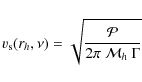
where

where I is the mode inertia (see Eq. (2) of Paper I),
In Sect. 2.2 we
will compare estimated values of ![]() with the seismic constraint obtained by Mosser
et al. (2005) with the HARPS spectrograph.
We therefore need to estimate
with the seismic constraint obtained by Mosser
et al. (2005) with the HARPS spectrograph.
We therefore need to estimate ![]() at the layer h where the
HARPS spectrograph is the most sensitive to the mode
displacement. As discussed by Samadi
et al. (2008a), the seismic measurements obtained
with HARPS spectrograph are likely to arise from the optical
depth
at the layer h where the
HARPS spectrograph is the most sensitive to the mode
displacement. As discussed by Samadi
et al. (2008a), the seismic measurements obtained
with HARPS spectrograph are likely to arise from the optical
depth ![]() ,
which corresponds to the depth where the potassium (K)
spectral
line is formed. We then compute the mode mass at the layer h
associated with the optical depth
,
which corresponds to the depth where the potassium (K)
spectral
line is formed. We then compute the mode mass at the layer h
associated with the optical depth
![]() (Christensen-Dalsgaard & Gough
1982). For the model with [Fe/H] = 0
(resp. [Fe/H] = -1) this optical depth
corresponds to h
(Christensen-Dalsgaard & Gough
1982). For the model with [Fe/H] = 0
(resp. [Fe/H] = -1) this optical depth
corresponds to h ![]() 390 km (resp. h
390 km (resp. h ![]() 350 km).
350 km).
For the mode linewidth ![]() we use the seismic measurement obtained from the seismic analysis of
the CoRoT data performed by Benomar
et al. (2009).
This seismic analysis combined the two CoRoT runs available
for
HD 49933. Two different approaches were considered in this
analysis: one based on the maximum likelihood estimator and the second
one using the Bayesian approach coupled with a Markov Chains
Monte Carlo algorithm. The Bayesian approach remains in
general
more reliable even in low signal-to-noise conditions. Nevertheless,
in terms of mode amplitudes, mode heights and mode linewidths,
both methods agree within 1-
we use the seismic measurement obtained from the seismic analysis of
the CoRoT data performed by Benomar
et al. (2009).
This seismic analysis combined the two CoRoT runs available
for
HD 49933. Two different approaches were considered in this
analysis: one based on the maximum likelihood estimator and the second
one using the Bayesian approach coupled with a Markov Chains
Monte Carlo algorithm. The Bayesian approach remains in
general
more reliable even in low signal-to-noise conditions. Nevertheless,
in terms of mode amplitudes, mode heights and mode linewidths,
both methods agree within 1-![]() .
We will consider here the seismic parameters and associated error bars
obtained on the basis of the Bayesian approach.
.
We will consider here the seismic parameters and associated error bars
obtained on the basis of the Bayesian approach.
![\begin{figure}
\par\hspace*{2mm}\includegraphics[width=8.2cm,clip]{11868fig1.eps}\vspace*{3mm}
\includegraphics[width=8.5cm,clip]{11868fig2.eps}
\end{figure}](/articles/aa/full_html/2010/01/aa11868-09/img27.png)
|
Figure 1:
Top: intrinsic mode surface velocity as a
function of the mode frequency ( |
| Open with DEXTER | |
2.2 Comparison with the HARPS measurements
The seismic analysis in velocity has been performed by Mosser et al. (2005)
using data from the HARPS spectrograph. The quality of these
data is too poor to perform a direct comparison
between the observed spectrum and the calculated amplitude
spectrum (![]() ,
Eq. (1)).
Indeed, the observed spectrum is highly affected by the day aliases.
Furthermore, the quality of the data does not allow to isolate
individual modes, in particular modes of a different angular
degree (
,
Eq. (1)).
Indeed, the observed spectrum is highly affected by the day aliases.
Furthermore, the quality of the data does not allow to isolate
individual modes, in particular modes of a different angular
degree (![]() ).
A consequence is that energies of modes which are close in
frequency are mixed.
).
A consequence is that energies of modes which are close in
frequency are mixed.
In order to measure the oscillation amplitude in a way that is
independent of these effects, we have
followed the method introduced by Kjeldsen
et al. (2005, see also Kjeldsen et al. 2008).
This method consists in deriving the oscillation amplitudes
from
the oscillation power density spectrum smoothed over typically four
times the large separation (i.e. four radial orders). Next, we
multiply this smoothed spectrum by a coefficient in order to convert
the apparent amplitudes into intrinsic
amplitudes. This coefficient takes into account the spatial response
function of the angular degrees ![]() = 0-3 (see Kjeldsen et al. 2008).
We have checked that the sensitivity of the visibility factor with the
limb-darkening law is significantly smaller in comparison with the
error associated with the Mosser
et al. (2005) seismic measurements. The amplitude
spectrum
= 0-3 (see Kjeldsen et al. 2008).
We have checked that the sensitivity of the visibility factor with the
limb-darkening law is significantly smaller in comparison with the
error associated with the Mosser
et al. (2005) seismic measurements. The amplitude
spectrum
![]() derived following Kjeldsen
et al. (2005) is shown in Fig. 1. The 1-
derived following Kjeldsen
et al. (2005) is shown in Fig. 1. The 1-![]() error
bar associated with each values of
error
bar associated with each values of
![]() is constant and equal to
is constant and equal to ![]() cm/s.
cm/s.
The maximum of ![]() reaches
reaches ![]()
![]() 7 cm/s. By comparison, Mosser
et al. (2005) found a maximum of 40
7 cm/s. By comparison, Mosser
et al. (2005) found a maximum of 40 ![]() 10 cm/s, which once converted into intrinsic
amplitude represents a maximum of 42
10 cm/s, which once converted into intrinsic
amplitude represents a maximum of 42 ![]() 10 cm/s. The difference between the two values is within the 1-
10 cm/s. The difference between the two values is within the 1-![]() error
bars. The different value found by Mosser
et al. (2005) can be explained by the way the
maximum of the mode amplitude was derived. Indeed, Mosser et al. (2005)
have constructed synthetic time series based on a theoretical low
degree p-modes eigenfrequency pattern and theoretical mode lines widths
(Houdek et al. 1999).
The maximum
amplitudes were assumed to follow a Gaussian distribution in frequency.
Using a Monte-Carlo approach, the maximum amplitude was then determined
in order to obtain comparable energy per frequency bin in the synthetic
and observed spectra. On the other hand, except for the mode response
function, the method by Kjeldsen
et al. (2005)
does not impose a priori constraints concerning the modes.
This
method can then be considered to be more reliable than the method by Mosser et al. (2005).
error
bars. The different value found by Mosser
et al. (2005) can be explained by the way the
maximum of the mode amplitude was derived. Indeed, Mosser et al. (2005)
have constructed synthetic time series based on a theoretical low
degree p-modes eigenfrequency pattern and theoretical mode lines widths
(Houdek et al. 1999).
The maximum
amplitudes were assumed to follow a Gaussian distribution in frequency.
Using a Monte-Carlo approach, the maximum amplitude was then determined
in order to obtain comparable energy per frequency bin in the synthetic
and observed spectra. On the other hand, except for the mode response
function, the method by Kjeldsen
et al. (2005)
does not impose a priori constraints concerning the modes.
This
method can then be considered to be more reliable than the method by Mosser et al. (2005).
We compare in Fig. 1 ![]() with the calculated mode surface velocity
with the calculated mode surface velocity ![]() (Eq. (1)).
However, in order to have a consistent comparison, we have
smoothed
(Eq. (1)).
However, in order to have a consistent comparison, we have
smoothed ![]() quadratically over four radial orders. We note
quadratically over four radial orders. We note ![]() the 1-
the 1-![]() error
bars associated with
error
bars associated with ![]() .
They are derived from
.
They are derived from
![]() ,
the 1-
,
the 1-![]() error
bars associated with
error
bars associated with ![]() .
As pointed out in Paper I, the uncertainty related to
our knowledge of the metal abundance Z for
HD 49933 results in an uncertainty about the determination
of
.
As pointed out in Paper I, the uncertainty related to
our knowledge of the metal abundance Z for
HD 49933 results in an uncertainty about the determination
of ![]() .
However, in terms of amplitude, this uncertainty is of the order
of 5%; this is negligible compared to the uncertainty
that
arises from
.
However, in terms of amplitude, this uncertainty is of the order
of 5%; this is negligible compared to the uncertainty
that
arises from
![]() (ranging between 25% to 50% in terms
of amplitude).
(ranging between 25% to 50% in terms
of amplitude).
The difference between computed values and observations is
shown in the bottom panel of Fig. 1. This
difference must be compared with ![]() ,
the 1-
,
the 1-![]() interval
resulting from the errors associated with
interval
resulting from the errors associated with ![]() and this in turn associated with
and this in turn associated with
![]() ,
that is
,
that is ![]() .
As seen in Fig. 1,
except at high frequency (
.
As seen in Fig. 1,
except at high frequency (
![]() mHz), the
theoretical
mHz), the
theoretical ![]() lie
well in the 1-
lie
well in the 1-![]() domain.
However, there is a clear disagreement at high frequencies
where
the computed mode surface velocities overestimate the observations.
This disagreement is attributed to the assumptions in the theoretical
model of stochastic excitation (see Sect. 4.5).
domain.
However, there is a clear disagreement at high frequencies
where
the computed mode surface velocities overestimate the observations.
This disagreement is attributed to the assumptions in the theoretical
model of stochastic excitation (see Sect. 4.5).
Assuming the 3D model with the solar abundance results in
significantly larger ![]() .
In that case the differences between computed
.
In that case the differences between computed ![]() and the seismic constraint are in general larger than 2-
and the seismic constraint are in general larger than 2-![]() .
This shows that ignoring the metal abundance of HD 49933 would
result in a larger discrepancy between
.
This shows that ignoring the metal abundance of HD 49933 would
result in a larger discrepancy between ![]() and
and
![]() .
.
3 Amplitudes of mode in intensity
3.1 Derivation of mode amplitudes in intensity
Fluctuations of the luminosity L due to variations
of the stellar radius can be neglected since we are looking at
high n order modes; accordingly the
bolometric mode intensity fluctuations ![]() are mainly due to variations of the effective temperature,
that is:
are mainly due to variations of the effective temperature,
that is:

As in Kjeldsen & Bedding (1995), we now assume that
where
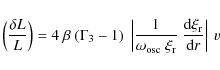
where v is computed using Eq. (1) with h = 0 (the photosphere), that is:
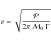
where
In Eq. (5),
![]() is a free
parameter introduced so that Eq. (5) gives,
in the case of the solar p modes, the correct maximum
in
is a free
parameter introduced so that Eq. (5) gives,
in the case of the solar p modes, the correct maximum
in
![]() .
Indeed, Eq. (5)
applied to the case of the solar p modes, overestimates by
.
Indeed, Eq. (5)
applied to the case of the solar p modes, overestimates by ![]() times
the mode amplitudes in intensity. This important discrepancy is mainly
a consequence of the adiabatic approximation.
times
the mode amplitudes in intensity. This important discrepancy is mainly
a consequence of the adiabatic approximation.
From the SOHO/GOLF seismic data (Baudin
et al. 2005), we derive the maximum of the solar
mode (intrinsic) surface velocity, that is 32.6 ![]() 2.6 cm/s. Then, using
2.6 cm/s. Then, using ![]() ,
we infer the
maximum of mode velocity at the photosphere, that is 18.5
,
we infer the
maximum of mode velocity at the photosphere, that is 18.5 ![]() 1.5 cm/s. According to Michel
et al. (2009), the maximum of the solar mode
(bolometric) amplitude in intensity is equal to
2.53
1.5 cm/s. According to Michel
et al. (2009), the maximum of the solar mode
(bolometric) amplitude in intensity is equal to
2.53 ![]() 0.11 ppm.
Then, by applying Eq. (5)
in the case of the Sun, we derive the scaling factor
0.11 ppm.
Then, by applying Eq. (5)
in the case of the Sun, we derive the scaling factor ![]()
![]() 10%. We have checked that this calibration depends very little on the
choice of the chemical mixture (see also Sect. 4.3).
We then adopt this value for the case of HD 49933.
10%. We have checked that this calibration depends very little on the
choice of the chemical mixture (see also Sect. 4.3).
We then adopt this value for the case of HD 49933.
3.2 The mode intensity fluctuations measured by CoRoT
The seismic analysis by Benomar
et al. (2009) provides the apparent
amplitude ![]() of the
of the ![]() = 0-2 modes
and the associated error bars. However, the CoRoT measurements
= 0-2 modes
and the associated error bars. However, the CoRoT measurements ![]() correspond to relative intensity fluctuations in the
CoRoT passband. Furthermore, the observed
(apparent) mode amplitudes depend on the degree
correspond to relative intensity fluctuations in the
CoRoT passband. Furthermore, the observed
(apparent) mode amplitudes depend on the degree ![]() .
Therefore, to transform them into bolometric
and intrinsic intensity fluctuations normalised
to the radial modes, we divide them by the CoRoT response
function,
.
Therefore, to transform them into bolometric
and intrinsic intensity fluctuations normalised
to the radial modes, we divide them by the CoRoT response
function, ![]() ,
derived here for
,
derived here for ![]() = 0-2,
following Michel et al.
(2009). The adopted values for
= 0-2,
following Michel et al.
(2009). The adopted values for ![]() are: R0=0.90, R1=1.10,
and R2=0.66. We finally
derive the bolometric intensity fluctuations normalised to the radial
modes according to:
are: R0=0.90, R1=1.10,
and R2=0.66. We finally
derive the bolometric intensity fluctuations normalised to the radial
modes according to:
|
(7) |
We shall stress that the differences between the amplitudes derived by Benomar et al. (2009) and by Appourchaux et al. (2008) are smaller than the 1-
3.3 Comparison with the CoRoT measurements
We compute the mode amplitudes in terms of bolometric intensity
fluctuations, ![]() ,
according to Eqs. (5)
and (6)
(see Sect. 3.1).
As for
,
according to Eqs. (5)
and (6)
(see Sect. 3.1).
As for ![]() ,
the uncertainty associated with the measured mode linewidths,
,
the uncertainty associated with the measured mode linewidths, ![]() ,
put uncertainties on the theoretical values of
,
put uncertainties on the theoretical values of
![]() .
Furthermore, the uncertainty associated with the calibrated
factor
.
Furthermore, the uncertainty associated with the calibrated
factor ![]() (see Sect. 3.1)
also puts an additional uncertainty on
(see Sect. 3.1)
also puts an additional uncertainty on
![]() .
From here on,
.
From here on, ![]() will refer to the 1-
will refer to the 1-![]() uncertainties
associated with
uncertainties
associated with ![]() .
Accordingly, we have
.
Accordingly, we have ![]() ,
where
,
where
![]() (reps.
(reps.
![]() )
is the 1-
)
is the 1-![]() uncertainty
associated with
uncertainty
associated with ![]() (resp.
(resp. ![]() ).
).
Figure 2
compares, as a function of the mode frequency, ![]() to
the CoRoT measurements:
to
the CoRoT measurements: ![]() .
The difference between our calculations and the observations is shown
in the bottom panel. As for the velocity, this difference must
be
compared with
.
The difference between our calculations and the observations is shown
in the bottom panel. As for the velocity, this difference must
be
compared with ![]() ,
the 1-
,
the 1-![]() interval
resulting from the association of the 1-
interval
resulting from the association of the 1-![]() error bars
error bars ![]() and the 1-
and the 1-![]() error,
error,
![]() ,
associated with the CoRoT measurements. Accordingly, we have
,
associated with the CoRoT measurements. Accordingly, we have ![]() where
where ![]() and
and ![]() .
.
As seen in Fig. 2, below ![]() mHz,
values of
mHz,
values of
![]() are within approximately 1-
are within approximately 1-![]() in agreement with
in agreement with ![]() .
However, above
.
However, above ![]() mHz,
the differences between
mHz,
the differences between
![]() and
and
![]() exceed 2-
exceed 2-![]() .
.
Assuming a solar abundance ([Fe/H] = 0)
results in a clear overestimation of ![]() .
Furthermore, calculations which assume the Grevesse
& Noels (1993) chemical mixture
result in mode amplitudes larger by
.
Furthermore, calculations which assume the Grevesse
& Noels (1993) chemical mixture
result in mode amplitudes larger by ![]() 15%.
15%.
Both in terms of intensity and velocity, differences between
the
calculated mode amplitudes and those derived from the observations
(CoRoT and HARPS) are approximately within the 1-![]() domain below
domain below ![]()
![]() 1.9 mHz. This then validates the intensity-velocity relation
given by Eq. (5)
at the level of the current seismic precision.
1.9 mHz. This then validates the intensity-velocity relation
given by Eq. (5)
at the level of the current seismic precision.
The maximum ![]() peaks at
peaks at ![]() mHz
and the maximum of
mHz
and the maximum of ![]() at
at ![]() mHz.
By comparison,
mHz.
By comparison, ![]() peaks
at
peaks
at ![]() mHz
and
mHz
and ![]() peaks at
peaks at ![]() mHz.
The difference in
mHz.
The difference in
![]() between the observations (CoRoT and HARPS) and the model can be
partially a
consequence of the clear tendency at high frequency toward
over-estimated amplitudes compared to the observations.
between the observations (CoRoT and HARPS) and the model can be
partially a
consequence of the clear tendency at high frequency toward
over-estimated amplitudes compared to the observations.
![\begin{figure}
\par\hspace*{2.5mm}\includegraphics[width=8.3cm,clip]{11868fig3.eps}\vspace*{3mm}
\includegraphics[width=8.5cm,clip]{11868fig4.eps}
\end{figure}](/articles/aa/full_html/2010/01/aa11868-09/img66.png)
|
Figure 2:
Top: mode bolometric amplitude in intensity
as a function of the mode frequency ( |
| Open with DEXTER | |
4 Discussion
4.1 Uncertainties in the knowledge of the fundamental parameters of HD 49933
Uncertainties in the knowledge of ![]() and
and ![]() place
uncertainties on the theoretical values of
place
uncertainties on the theoretical values of ![]() and hence on the mode amplitudes (
and hence on the mode amplitudes (![]() and
and
![]() ). However, estimating these
uncertainties would require the consideration of 3D models
with a
). However, estimating these
uncertainties would require the consideration of 3D models
with a
![]() and a
and a ![]() that depart more than 1-
that depart more than 1-![]() from the values adopted in our modeling, i.e.
from the values adopted in our modeling, i.e.
![]() K and
K and ![]() .
This is beyond the scope of our efforts since such
3D models are not yet available.
.
This is beyond the scope of our efforts since such
3D models are not yet available.
4.2 Influence of the mode mass
As discussed in details in Samadi
et al. (2008a), the computed mode surface
velocities ![]() significantly depend on the choice of the height h
in the atmosphere where the mode masses are evaluated. According to Samadi et al. (2008a),
seismic measurements performed with the HARPS spectrograph
reflect
conditions slightly below the formation depth of the K line.
Accordingly, we have evaluated by default the mode masses at the
optical depth where the K line is expected to be formed
(i.e.
significantly depend on the choice of the height h
in the atmosphere where the mode masses are evaluated. According to Samadi et al. (2008a),
seismic measurements performed with the HARPS spectrograph
reflect
conditions slightly below the formation depth of the K line.
Accordingly, we have evaluated by default the mode masses at the
optical depth where the K line is expected to be formed
(i.e.
![]() ),
which corresponds, for our 3D models, to a height of
about
350 km above the photosphere. We can evaluate how sensitive we
are to the choice of h. Indeed, evaluating
the mode mass at the photosphere results in values of
),
which corresponds, for our 3D models, to a height of
about
350 km above the photosphere. We can evaluate how sensitive we
are to the choice of h. Indeed, evaluating
the mode mass at the photosphere results in values of ![]() which
are about 15% lower and hence would reduce the discrepancy
with
the HARPS observations. On the other hand, evaluating the mode
mass one pressure scale height (
which
are about 15% lower and hence would reduce the discrepancy
with
the HARPS observations. On the other hand, evaluating the mode
mass one pressure scale height (![]() 300 km at the photosphere) above h
=
350 km results in an increase of
300 km at the photosphere) above h
=
350 km results in an increase of ![]() of about 10%. A more rigorous approach to derive the
different heights in the atmosphere where the measurements are
sensitive would require a dedicated modeling (see a discussion
in Samadi et al. 2008a).
of about 10%. A more rigorous approach to derive the
different heights in the atmosphere where the measurements are
sensitive would require a dedicated modeling (see a discussion
in Samadi et al. 2008a).
4.3 The intensity-velocity relation
Sensitivity to the location:
the derivation of Eq. (4) (or equivalently Eq. (5)) is based on the assumption thatNon-adiabatic effects:
the modes are measured at the surface of the star where non-adiabatic interactions between the modes and convection as well as radiative losses of the modes are important. Assuming Eq. (4) is then a crude approximation. In fact, it is clearly non-valid in the case of the Sun since it results in a severe over-estimation of the solar mode amplitudes in intensity (see Sect. 3.1). Avoiding this approximation requires non-adiabatic eigenfunctions computed with a time-dependent convection model. However, such models (e.g. Balmforth 1992; Grigahcène et al. 2005) are subject to large uncertainties, and there is currently no consensus about the non-adiabatic mechanisms that play a significant role (see e.g. the recent review by Houdek 2008). For instance, parameters are usually introduced in the theories so that they cannot be used in a predictive way.In the present study, we adopt by default the adiabatic
approximation and introduce in Eq. (5) the
parameter ![]() calibrated with helioseismic data. We show here that despite the
deficiency of the quasi-adiabatic approximation, it nevertheless
provides the correct scaling, at least at low frequency and at
the
level of the present seismic precisions.
calibrated with helioseismic data. We show here that despite the
deficiency of the quasi-adiabatic approximation, it nevertheless
provides the correct scaling, at least at low frequency and at
the
level of the present seismic precisions.
As an alternative approach, comparing the spectrum obtained from the 3D models in intensity with that obtained in velocity can provide valuable information concerning the intensity-velocity relation, in particular concerning the departure from the adiabatic approximation and the sensitivity to the surface metal abundance. We have started to carry out such a study. For the velocity, the (few) acoustic modes trapped in the simulated boxes can be extracted and their properties measured. But this was impossible to do for the intensity with the simulations at our disposal because the computed spectrum for the intensity is dominated by the granulation background. As a consequence it is not possible to extract the mode amplitudes in intensity with sufficient accuracy. A comparison between the spectra obtained from the 3D models requires a much longer time series (work in progress).
Sensitivity to the metal abundance:
we have shown in this study how the mode amplitudes in the velocity are sensitive to the surface metal abundance. An open question is how sensitive is the intensity-velocity relation in general to the metal abundance? A theoretical answer to this question would require a realistic and validated non-adiabatic treatment. The pure numerical approach mentionned above can also in principle provide some answers to this question. However, as discussed above, this approach is not applicable with the time series at our disposal. Concerning the quasi-adiabatic relation of Eq. (5): a change of the metal abundance has a direct effect on4.4 The solar case
As seen in this study, the surface metal abundance has a pronounced effect on the mode excitation rates. One may then wonder about the previous validation of the theoretical model of stochastic excitation in the case of the Sun (Belkacem et al. 2006; Samadi et al. 2008b). Indeed, this validation was carried out with the use of a solar 3D model based on an ``old'' solar chemical mixture (namely those proposed by Anders & Grevesse 1989) while the ``new'' chemical mixture by Asplund et al. (2005) is characterized by a significantly lower metal abundance.
In order to adress this issue, we have first considered two
global
1D solar models. One model has an ``old'' solar abundance (Grevesse & Noels 1993,
model
![]() hereafter) while the second one has the ``new'' abundances (Asplund et al. 2005,
model
hereafter) while the second one has the ``new'' abundances (Asplund et al. 2005,
model
![]() hereafter). At the surface where the excitation occurs, the
density of the solar model
hereafter). At the surface where the excitation occurs, the
density of the solar model
![]() is only
is only ![]() 5%
lower
compared to the model
5%
lower
compared to the model
![]() .
According to the arguments developed in Paper I, this
difference
in the density must imply a difference in the convective
velocities (
.
According to the arguments developed in Paper I, this
difference
in the density must imply a difference in the convective
velocities (![]() )
of the
order of
)
of the
order of ![]() ,
where
,
where
![]() (resp.
(resp.
![]() )
is the surface density associated with
)
is the surface density associated with
![]() (resp.
(resp.
![]() ). Accordingly,
). Accordingly, ![]() is
expected to be
is
expected to be ![]() 1.7% higher
for
1.7% higher
for
![]() compared to
compared to
![]() .
.
The next question is what is the change in the solar mode
excitation rates induced by the above difference in ![]() ?
We have computed the solar mode excitation rates exactly in the same
manner as for HD 49333 by using a solar
3D simulations based
on the ``old'' abundances. We obtained a rather good agreement with the
different helioseismic data (see the result in Samadi
et al. 2008b).
To derive the solar mode excitations expected with the ``new''
solar abudance, we have proceeded in a similar way as the one done in
Paper I: we have increased the convective velocity
?
We have computed the solar mode excitation rates exactly in the same
manner as for HD 49333 by using a solar
3D simulations based
on the ``old'' abundances. We obtained a rather good agreement with the
different helioseismic data (see the result in Samadi
et al. 2008b).
To derive the solar mode excitations expected with the ``new''
solar abudance, we have proceeded in a similar way as the one done in
Paper I: we have increased the convective velocity ![]() derived from the solar 3D model by 2% while keeping
the
kinetic flux constant (see details in Paper I). This
increase
of
derived from the solar 3D model by 2% while keeping
the
kinetic flux constant (see details in Paper I). This
increase
of ![]() 2% of
2% of ![]() results
in an increase of
results
in an increase of ![]() 10%
of the mode excitation rates. This increase is significantly lower than
the current uncertainties associated with the different helioseismic
data (Baudin
et al. 2005; Samadi et al. 2008b).
10%
of the mode excitation rates. This increase is significantly lower than
the current uncertainties associated with the different helioseismic
data (Baudin
et al. 2005; Samadi et al. 2008b).
4.5 Discrepancy at high frequency
The discrepancy betwen theoretical calculations and observations is particularly pronounced at high frequency. This discrepancy may be attributed to a canceling between the entropy and the Reynolds stress contributions (see Sect. 4.5.1) or the ``scale length separation'' assumption (see Sect. 4.5.2).
4.5.1 Canceling between the entropy and the Reynolds stress contributions
The relative contribution of the entropy fluctuations to the excitation
is found to be about 30% of the total excitation. This is two
times larger than in the case of the Sun (![]() 15%). This can be explained by the fact
HD 49933 is significantly hotter than the Sun and, as
pointed-out by Samadi
et al. (2007), the larger
15%). This can be explained by the fact
HD 49933 is significantly hotter than the Sun and, as
pointed-out by Samadi
et al. (2007), the larger ![]() ,
the more important the relative contribution of the entropy. Although
more important than in the Sun, the contribution of the entropy
fluctuations remains relatively smaller than the uncertainties
associated with the current seismic data. This is illustrated
in
Fig. 3:
the difference between theoretical mode amplitudes which take
into account only the Reynolds stress contribution (
,
the more important the relative contribution of the entropy. Although
more important than in the Sun, the contribution of the entropy
fluctuations remains relatively smaller than the uncertainties
associated with the current seismic data. This is illustrated
in
Fig. 3:
the difference between theoretical mode amplitudes which take
into account only the Reynolds stress contribution (
![]() ,
see Eq. (3) of Paper I) and those that
include both
contributions (entropy and Reynolds stress) is lower than
,
see Eq. (3) of Paper I) and those that
include both
contributions (entropy and Reynolds stress) is lower than ![]() .
In terms of amplitudes, the entropy fluctuations contribute
only
.
In terms of amplitudes, the entropy fluctuations contribute
only ![]() 15%
of the global amplitude. This is significantly smaller than the
uncertainties associated with the current seismic measurements. Seismic
data of a better quality are then needed to constrain the entropy
contribution and its possible canceling with the
Reynolds stress.
15%
of the global amplitude. This is significantly smaller than the
uncertainties associated with the current seismic measurements. Seismic
data of a better quality are then needed to constrain the entropy
contribution and its possible canceling with the
Reynolds stress.
Numerical simulations show some cancellation between the entropy source term and the one due to the Reynolds stress (Stein et al. 2004). However, in the present theoretical model of stochastic excitation, the cross terms between the entropy fluctuations and the Reynolds stresses vanish (see Samadi & Goupil 2001). This is a consequence of the different assumptions concerning the entropy fluctuations (see Samadi & Goupil 2001; see also the recent discussion in Samadi et al. 2008b). Accordingly, the entropy source term is included as a source independent from the Reynolds stress contribution. As suggested by Houdek (2006), a partial canceling between the entropy fluctuations and the Reynolds stress can decrease the mode amplitudes of F-type stars and reduce the discrepancy between the theoretical calculations and the observations.
![\begin{figure}
\par\hspace*{-1mm}\includegraphics[width=8.5cm,clip]{11868fig5.eps}\vspace*{3mm}
\includegraphics[width=8.4cm,clip]{11868fig6.eps}
\end{figure}](/articles/aa/full_html/2010/01/aa11868-09/img91.png)
|
Figure 3:
Top: same as Fig. 1.
The thin dashed line corresponds to a calculation that takes only the
contribution of the Reynolds stress into account. The dot-dashed line
corresponds to a calculation in which we have assumed that the
contribution of the Reynolds stress interferes totally with that of the
entropy fluctuations (see text). The thick solid line has the
same
meaning as in Fig. 1.
Bottom: same as top for
|
| Open with DEXTER | |
There is currently no theoretical description of these interferences.
In order to have an upper limit of the interferences, we assume that
both contributions locally and fully
interfer. This assumption leads to the computation of the excitation
rates per unit mass as:
where
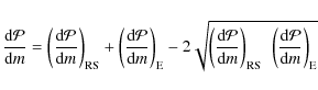
We have assumed here that the cancellation between the two terms is independent of the mode frequency (see Eq. (8)). However, according to Stein et al. (2004), the level of the cancellation depends on the frequency (see their Fig. 8). In particular, for F-type stars, the cancellation is expected to be more important around and above the peak frequency.
As a conclusion, the existence of a partial canceling between the entropy fluctuations and the Reynolds stress can decrease the mode amplitude and could improve the agreement with the seismic observations at high frequency. However, there is currently no theoretical modeling of the interference between theses two terms. Further theoretical developements are required.
4.5.2 The ``scale length separation'' assumption
The ``scale length separation'' assumption (see the review by Samadi et al. 2008b)
consists of the assumption that the eddies contributing effectively to
the driving have a characteristic length scale smaller than the mode
wavelength. This assumption is justified for a low Mach
number (![]() ).
However, this approximation is less valid in the super-adiabatic region
where
).
However, this approximation is less valid in the super-adiabatic region
where ![]() reaches a maximum (for the Sun
reaches a maximum (for the Sun ![]() is up to 0.3) and accordingly affects the high-frequency modes
more. This approximation is then expected to be even more questionable
for stars hotter than the Sun, since
is up to 0.3) and accordingly affects the high-frequency modes
more. This approximation is then expected to be even more questionable
for stars hotter than the Sun, since ![]() increases with
increases with
![]() .
This spatial separation can be avoided, however if the kinetic
energy spectrum associated with the turbulent elements (E(k))
is properly coupled with the spatial dependence of the modes
(work in progress). In that case, we expect a more
rapid
decrease of the driving efficiency with increasing frequency than in
the present formalism where the spatial dependence of the modes is
totally decoupled from E(k)
(i.e. ``scale length separation'').
.
This spatial separation can be avoided, however if the kinetic
energy spectrum associated with the turbulent elements (E(k))
is properly coupled with the spatial dependence of the modes
(work in progress). In that case, we expect a more
rapid
decrease of the driving efficiency with increasing frequency than in
the present formalism where the spatial dependence of the modes is
totally decoupled from E(k)
(i.e. ``scale length separation'').
5 Conclusion
From the mode linewidths measured by CoRoT and theoretical mode
excitation rates derived for HD 49933, we have derived the
expected mode surface velocities ![]() which we have compared with
which we have compared with
![]() ,
the mode velocity spectrum derived from the seismic observations
obtained with the HARPS spectrograph (Mosser
et al. 2005). Except at high frequency (
,
the mode velocity spectrum derived from the seismic observations
obtained with the HARPS spectrograph (Mosser
et al. 2005). Except at high frequency (![]()
![]() 1.9 mHz),
the agreement between computed
1.9 mHz),
the agreement between computed ![]() and
and
![]() is within the 1-
is within the 1-![]() domain
associated with the seismic data from the HARPS spectrograph.
However, there is a clear tendency to overestimate
domain
associated with the seismic data from the HARPS spectrograph.
However, there is a clear tendency to overestimate
![]() above
above ![]()
![]() 1.9 mHz.
1.9 mHz.
Using a calibrated quasi-adiabatic
approximation to relate the mode velocity to the mode
amplitude in intensity (Eq. (5)),
we have derived for the case of HD 49933 the expected
mode
amplitudes in intensity. Computed mode intensity fluctuations,
![]() ,
are within 1-
,
are within 1-![]() in agreement with the seismic constraints derived from the
CoRoT data (Benomar
et al. 2009). However, as for the velocity, there is
a clear tendency at high frequency (
in agreement with the seismic constraints derived from the
CoRoT data (Benomar
et al. 2009). However, as for the velocity, there is
a clear tendency at high frequency (![]()
![]() 1.9 mHz) towards
over-estimated
1.9 mHz) towards
over-estimated ![]() compared to the CoRoT observations.
compared to the CoRoT observations.
Calculations that assume a solar surface metal abundance
result, both in velocity and in intensity, in amplitudes larger by ![]() 35% around
the peak frequency (
35% around
the peak frequency (
![]()
![]() 1.8 mHz) and by up to a factor of two at lower frequency.
It follows that, ignoring the current surface metal abundance
of
the star results in a more severe over-estimation of the computed
amplitudes compared with observations. This illustrates the importance
of taking the surface metal abundance of the solar-like pulsators into
account when modeling the mode driving. In addition, we point
out
that the Grevesse & Noels (1993)
solar chemical mixture results in mode amplitudes larger by
about 15% with respect to calculations that assume the ``new''
solar abundance by Asplund
et al. (2005). However, this increase remains
significantly smaller than the uncertainties associated with current
seismic measurements.
1.8 mHz) and by up to a factor of two at lower frequency.
It follows that, ignoring the current surface metal abundance
of
the star results in a more severe over-estimation of the computed
amplitudes compared with observations. This illustrates the importance
of taking the surface metal abundance of the solar-like pulsators into
account when modeling the mode driving. In addition, we point
out
that the Grevesse & Noels (1993)
solar chemical mixture results in mode amplitudes larger by
about 15% with respect to calculations that assume the ``new''
solar abundance by Asplund
et al. (2005). However, this increase remains
significantly smaller than the uncertainties associated with current
seismic measurements.
Since both mode amplitudes in terms of surface velocity and intensity are available for this star, it was possible to test the validity of the calibrated quasi-adiabatic relation (Eq. (5)). Our comparison shows that this relation provides the correct scaling, at least at the level of the present seismic precisions.
Both in terms of surface velocity and of intensity, the
differences between predicted and observed mode amplitudes are within
the 1-![]() uncertainty
domain, except at high frequency. This result then validates for low
frequency modes the basic underlying physical assumptions included in
the theoretical model of stochastic excitation for a star significantly
different in effective temperature, surface gravity, turbulent Mach
number (
uncertainty
domain, except at high frequency. This result then validates for low
frequency modes the basic underlying physical assumptions included in
the theoretical model of stochastic excitation for a star significantly
different in effective temperature, surface gravity, turbulent Mach
number (![]() )
and metallicity compared to the
Sun or
)
and metallicity compared to the
Sun or ![]() Cen A.
Cen A.
As discussed in Sect. 4, the clear discrepancy between predicted and observed mode amplitudes seen at high frequency may have two possible origins: first, a canceling between the entropy contribution and the Reynolds stress is expected to occur and to be important around and above the frequency of the maximum of the mode excitation rates (see Sect. 4.5.1). Second, the assumption called the ``scale length separation'' (Samadi et al. 2008b) may also result in an over-estimation of the mode amplitudes at high frequency (see Sect. 4.5.2). These issues will be investigated in a forthcoming paper.
AcknowledgementsThe CoRoT space mission, launched on December 27 2006, has been developed and is operated by CNES, with the contribution of Austria, Belgium, Brasil, ESA, Germany and Spain. We are grateful to the referee for his pertinent comments. We are indebted to J. Leibacher for his careful reading of the manuscript. K.B. acknowledged financial support from Liège University through the Subside Fédéral pour la Recherche 2009.
References
- Anders, E., & Grevesse, N. 1989, Geochim. Cosmochim. Acta, 53, 197 [Google Scholar]
- Appourchaux, T., Michel, E., Auvergne, M., et al. 2008, A&A, 488, 705 [Google Scholar]
- Asplund, M., Grevesse, N., & Sauval, A. J. 2005, in Cosmic Abundances as Records of Stellar Evolution and Nucleosynthesis, ed. T. G. Barnes, III, & F. N. Bash, ASP Conf. Ser., 336, 25 [Google Scholar]
- Balmforth, N. J. 1992, MNRAS, 255, 603 [NASA ADS] [CrossRef] [Google Scholar]
- Baudin, F., Samadi, R., Goupil, M.-J., et al. 2005, A&A, 433, 349 [Google Scholar]
- Belkacem, K., Samadi, R., Goupil, M. J., Kupka, F., & Baudin, F. 2006, A&A, 460, 183 [Google Scholar]
- Benomar, O., Baudin, F., Campante, T., et al. 2009, A&A, 507, L13 [Google Scholar]
- Christensen-Dalsgaard, J., & Gough, D. O. 1982, MNRAS, 198, 141 [NASA ADS] [CrossRef] [Google Scholar]
- Grevesse, N., & Noels, A. 1993, in Origin and Evolution of the Elements, ed. N. Prantzos, E. Vangioni-Flam, & M. Cassé (Cambridge University Press), 15 [Google Scholar]
- Grigahcène, A., Dupret, M.-A., Gabriel, M., Garrido, R., & Scuflaire, R. 2005, A&A, 434, 1055 [Google Scholar]
- Houdek, G. 2006, in Proceedings of SOHO 18/GONG 2006/HELAS I, Beyond the spherical Sun, Published on CDROM, ESA SP, 624, 28.1 [Google Scholar]
- Houdek, G. 2008, Commun. Asteroseismol., 157, 137 [NASA ADS] [Google Scholar]
- Houdek, G., Balmforth, N. J., Christensen-Dalsgaard, J., & Gough, D. O. 1999, A&A, 351, 582 [Google Scholar]
- Kjeldsen, H., & Bedding, T. R. 1995, A&A, 293, 87 [Google Scholar]
- Kjeldsen, H., Bedding, T. R., Butler, R. P., et al. 2005, ApJ, 635, 1281 [NASA ADS] [CrossRef] [Google Scholar]
- Kjeldsen, H., Bedding, T. R., Arentoft, T., et al. 2008, ApJ, 682, 1370 [NASA ADS] [CrossRef] [Google Scholar]
- Michel, E., Baglin, A., Auvergne, M., et al. 2008, Science, 322, 558 [NASA ADS] [CrossRef] [PubMed] [Google Scholar]
- Michel, E., Samadi, R., Baudin, F., et al. 2009, A&A, 495, 979 [Google Scholar]
- Mosser, B., Bouchy, F., Catala, C., et al. 2005, A&A, 431, L13 [Google Scholar]
- Samadi, R., & Goupil, M. . 2001, A&A, 370, 136 [Google Scholar]
- Samadi, R., Georgobiani, D., Trampedach, R., et al. 2007, A&A, 463, 297 [Google Scholar]
- Samadi, R., Belkacem, K., Goupil, M. J., Dupret, M.-A., & Kupka, F. 2008a, A&A, 489, 291 [Google Scholar]
- Samadi, R., Belkacem, K., Goupil, M.-J., Ludwig, H.-G., & Dupret, M.-A. 2008b, Commun. Asteroseismol., 157, 130 [NASA ADS] [Google Scholar]
- Samadi, R., Ludwig, H.-G., Belkacem, K., Goupil, M., & Dupret, M.-A. 2010, A&A, 509, A15 (Paper I) [Google Scholar]
- Stein, R., Georgobiani, D., Trampedach, R., Ludwig, H.-G., & Nordlund, Å. 2004, Sol. Phys., 220, 229 [NASA ADS] [CrossRef] [Google Scholar]
Footnotes
- ... HD 49933
- The CoRoT space mission, launched on December 27 2006, has been developped and is operated by CNES, with the contribution of Austria, Belgium, Brasil, ESA, Germany and Spain.
All Figures
|
|
Figure 1:
Top: intrinsic mode surface velocity as a
function of the mode frequency ( |
| Open with DEXTER | |
| In the text | |
|
|
Figure 2:
Top: mode bolometric amplitude in intensity
as a function of the mode frequency ( |
| Open with DEXTER | |
| In the text | |
|
|
Figure 3:
Top: same as Fig. 1.
The thin dashed line corresponds to a calculation that takes only the
contribution of the Reynolds stress into account. The dot-dashed line
corresponds to a calculation in which we have assumed that the
contribution of the Reynolds stress interferes totally with that of the
entropy fluctuations (see text). The thick solid line has the
same
meaning as in Fig. 1.
Bottom: same as top for
|
| Open with DEXTER | |
| In the text | |
Copyright ESO 2010
Current usage metrics show cumulative count of Article Views (full-text article views including HTML views, PDF and ePub downloads, according to the available data) and Abstracts Views on Vision4Press platform.
Data correspond to usage on the plateform after 2015. The current usage metrics is available 48-96 hours after online publication and is updated daily on week days.
Initial download of the metrics may take a while.