| Issue |
A&A
Volume 509, January 2010
|
|
|---|---|---|
| Article Number | A15 | |
| Number of page(s) | 7 | |
| Section | Stellar structure and evolution | |
| DOI | https://doi.org/10.1051/0004-6361/200911867 | |
| Published online | 12 January 2010 | |
The CoRoT![[*]](/icons/foot_motif.png) target HD 49933
target HD 49933
I. Effect of the metal abundance on the mode excitation rates
R. Samadi1 - H.-G. Ludwig2 - K. Belkacem1,3 - M. J. Goupil1 - M.-A. Dupret1,3
1 - Observatoire de Paris, LESIA, CNRS UMR 8109,
Université Pierre et Marie Curie, Université Denis Diderot, 5 pl. J.
Janssen, 92195 Meudon, France
2 -
Observatoire de Paris, GEPI, CNRS UMR 8111, 5 pl. J. Janssen, 92195 Meudon, France
3 -
Institut d'Astrophysique et de Géophysique de l'Université de Liège,
Allée du 6 Août 17, 4000 Liège, Belgium
Received 17 February 2009 / Accepted 27 October 2009
Abstract
Context. Solar-like oscillations are stochastically excited by turbulent convection at the surface layers of the stars.
Aims. We study the role of the surface metal abundance on the
efficiency of the stochastic driving in the case of the CoRoT target
HD 49933.
Methods. We compute two 3D hydrodynamical simulations
representative - in effective temperature and gravity - of
the surface layers of the CoRoT target HD 49933, a star that is
rather metal poor and significantly hotter than the Sun. One 3D
simulation has a solar metal abundance, and the other has a surface
iron-to-hydrogen, [Fe/H], abundance ten times smaller. For each 3D
simulation we match an associated global 1D model, and we compute the
associated acoustic modes using a theoretical model of stochastic
excitation validated in the case of the Sun and ![]() Cen A.
Cen A.
Results. The rate at which energy is supplied per unit time into
the acoustic modes associated with the 3D simulation with
[Fe/H] = -1 is found to be about three times smaller than
those associated with the 3D simulation with [Fe/H] = 0. As shown here,
these differences are related to the fact that low metallicity implies
surface layers with a higher mean density. In turn, a higher mean
density favors smaller convective velocities and hence less efficient
driving of the acoustic modes.
Conclusions. Our result shows the importance of taking the
surface metal abundance into account in the modeling of the mode
driving by turbulent convection. A comparison with observational data
is presented in a companion paper using seismic data obtained for the
CoRoT target HD 49933.
Key words: convection - turbulence - stars: oscillations - stars: individual: HD 49933 - Sun: helioseismology
1 Introduction
Using the measured linewidths and the amplitudes of the solar acoustic modes,
it has been possible to infer the rate at which energy
is supplied per unit time into the solar acoustic modes. Using these constraints,
different models of mode excitation by turbulent
convection have been extensively tested in the case of the Sun (see
e.g. recent reviews by Samadi et al. 2008b; and Houdek 2006).
Among the different approaches, we can distinguish pure theoretical
approaches (e.g. Samadi & Goupil 2001; Chaplin et al. 2005), semi-analytical approaches (e.g. Samadi et al. 2003a,b) and pure numerical approaches (e.g. Nordlund & Stein 2001; Stein et al. 2004; Jacoutot et al. 2008).
The advantage of a theoretical approach is that it easily allows
massive computation of the mode excitation rates for a wide variety
of stars with different fundamental parameters (e.g. effective
temperature, gravity) and different surface metal abundance.
However, pure theoretical approaches are based on crude or simplified descriptions
of turbulent convection.
On the other hand, a semi-analytical approach is generally more
realistic since the quantities related to turbulent convection
are obtained from 3D hydrodynamical simulation.
3D hydrodynamical simulations are at this point in time too time consuming, so
that a fine grid of 3D models with a sufficient resolution in effective temperature (
![]() ), gravity (
), gravity (![]() )
and surface metal abundance (Z) is not yet available.
In the present paper, we study and provide a procedure to interpolate
for any value of Z the mode excitation
rates
)
and surface metal abundance (Z) is not yet available.
In the present paper, we study and provide a procedure to interpolate
for any value of Z the mode excitation
rates ![]() between two 3D simulations with
different Z but the same
between two 3D simulations with
different Z but the same
![]() and
and ![]() .
With such interpolation procedure it is no longer required to have at
our disposal a fine grid in Z of 3D simulations.
.
With such interpolation procedure it is no longer required to have at
our disposal a fine grid in Z of 3D simulations.
The semi-analytical mode that we consider here is based on Samadi & Goupil (2001)'s
theoretical model with the improvements proposed by Belkacem et al. (2006a). This semi-analytical model satisfactorily reproduces the solar seismic data
(Samadi et al. 2003a; Belkacem et al. 2006b). Recently, the seismic constraints obtained for ![]() Cen A (HD 128620) have provided an additional validation of the basic physical
assumptions of this theoretical model (Samadi et al. 2008a). The star
Cen A (HD 128620) have provided an additional validation of the basic physical
assumptions of this theoretical model (Samadi et al. 2008a). The star ![]() Cen A has a surface gravity (
Cen A has a surface gravity (
![]() )
lower than that of the Sun (
)
lower than that of the Sun (
![]() ), but its
effective temperature (
), but its
effective temperature (
![]() K) does not
significantly differ from that of the Sun (
K) does not
significantly differ from that of the Sun (
![]() K).
The higher
K).
The higher
![]() ,
the more vigorous the convective
velocity at the surface and the stronger the driving by turbulent
convection (see e.g. Houdek et al. 1999).
For main sequence stars with a mass
,
the more vigorous the convective
velocity at the surface and the stronger the driving by turbulent
convection (see e.g. Houdek et al. 1999).
For main sequence stars with a mass
![]() ,
an increase of the
convective velocity is expected to be associated with a larger turbulent
Mach number,
,
an increase of the
convective velocity is expected to be associated with a larger turbulent
Mach number, ![]() (Houdek et al. 1999). However, the theoretical models of stochastic excitation are
strictly valid in a medium where
(Houdek et al. 1999). However, the theoretical models of stochastic excitation are
strictly valid in a medium where ![]() is - as
in the Sun and
is - as
in the Sun and ![]() Cen A - rather small. Hence, the higher
Cen A - rather small. Hence, the higher ![]() ,
the more
questionable the different approximations and the assumptions involved in the
theory (see e.g. Samadi & Goupil 2001).
It is therefore important to test the theory with another star characterized by a
,
the more
questionable the different approximations and the assumptions involved in the
theory (see e.g. Samadi & Goupil 2001).
It is therefore important to test the theory with another star characterized by a
![]() significantly higher
than in the Sun.
significantly higher
than in the Sun.
Furthermore, the star ![]() Cen A has an iron-to-hydrogen abundance slightly
larger than the Sun, namely [Fe/H] = 0.2 (see Neuforge-Verheecke & Magain 1997). However, the modeling performed by Samadi et al. (2008a) for
Cen A has an iron-to-hydrogen abundance slightly
larger than the Sun, namely [Fe/H] = 0.2 (see Neuforge-Verheecke & Magain 1997). However, the modeling performed by Samadi et al. (2008a) for ![]() Cen A assumes a solar iron abundance ([Fe/H] = 0).
According to Houdek et al. (1999), the mode amplitudes are expected to
change with the metal abundance. However, Houdek et al. (1999)'s
result was obtained on the basis of a mixing-length approach involving
several free parameters and by using a theoretical model of
stochastic excitation in which a free multiplicative factor is
introduced in
order to reproduce the maximum of the solar mode excitation rates.
Therefore, it is important to extend Houdek et al. (1999)'s study by using
a more realistic modeling based on 3D hydrodynamical simulation of
the surface layers of stars and a theoretical model of mode driving
that reproduces - without the introduction of free parameters - the
available seismic constraints.
Cen A assumes a solar iron abundance ([Fe/H] = 0).
According to Houdek et al. (1999), the mode amplitudes are expected to
change with the metal abundance. However, Houdek et al. (1999)'s
result was obtained on the basis of a mixing-length approach involving
several free parameters and by using a theoretical model of
stochastic excitation in which a free multiplicative factor is
introduced in
order to reproduce the maximum of the solar mode excitation rates.
Therefore, it is important to extend Houdek et al. (1999)'s study by using
a more realistic modeling based on 3D hydrodynamical simulation of
the surface layers of stars and a theoretical model of mode driving
that reproduces - without the introduction of free parameters - the
available seismic constraints.
To this end, the star HD 49933 is an interesting
case for three reasons: first, this star has
![]() K (Bruntt et al. 2008),
K (Bruntt et al. 2008),
![]() (Bruntt et al. 2008) and [Fe/H]
(Bruntt et al. 2008) and [Fe/H]
![]() dex (Gillon & Magain 2006; Solano et al. 2005).
The properties of its surface layers are thus significantly different from
those of the Sun and
dex (Gillon & Magain 2006; Solano et al. 2005).
The properties of its surface layers are thus significantly different from
those of the Sun and ![]() Cen A. Second, HD 49933 was observed in Doppler velocity with the
HARPS spectrograph. A seismic analysis of these data performed by
Mosser et al. (2005) has provided the maximum of the mode surface velocity
(
Cen A. Second, HD 49933 was observed in Doppler velocity with the
HARPS spectrograph. A seismic analysis of these data performed by
Mosser et al. (2005) has provided the maximum of the mode surface velocity
(
![]() ).
Third, the star was more recently observed continuously in intensity by
CoRoT during 62 days. Apart from observations for the
Sun, this is the longest seismic observation ever peformed both from
the ground and from space. This long term and continuous observation provides a very high
frequency resolution (
).
Third, the star was more recently observed continuously in intensity by
CoRoT during 62 days. Apart from observations for the
Sun, this is the longest seismic observation ever peformed both from
the ground and from space. This long term and continuous observation provides a very high
frequency resolution (![]()
![]() Hz). The seismic analysis of these
observations undertaken by Appourchaux et al. (2008) or more recently by Benomar et al. (2009) have provided the direct measurements of the mode amplitudes and the
mode linewidths with an accuracy not previously achieved for a star other than the Sun.
Hz). The seismic analysis of these
observations undertaken by Appourchaux et al. (2008) or more recently by Benomar et al. (2009) have provided the direct measurements of the mode amplitudes and the
mode linewidths with an accuracy not previously achieved for a star other than the Sun.
We consider two 3D hydrodynamical simulations
representative - in effective temperature and gravity - of the
surface layers of HD 49933. One 3D simulation has [Fe/H] = 0, while the
second has [Fe/H] = -1. For each 3D simulation, we match an associated global 1D
model and compute the associated acoustic modes and mode excitation
rates, ![]() .
This permits us to quantify the variation of
.
This permits us to quantify the variation of
![]() induced by a change of the surface metal abundance Z.
From these two sets of calculation, we then deduce
induced by a change of the surface metal abundance Z.
From these two sets of calculation, we then deduce ![]() for
HD 49933 by taking into account the observed iron abundance of the
star (i.e. [Fe/H] = -0.37). In a companion paper (Samadi et al. 2010, hereafter Paper II), we will use these theoretical calculations of
for
HD 49933 by taking into account the observed iron abundance of the
star (i.e. [Fe/H] = -0.37). In a companion paper (Samadi et al. 2010, hereafter Paper II), we will use these theoretical calculations of ![]() and the mode linewidths obtained from the seismic analysis of HD 49933
performed with the CoRoT data to derive the expected mode amplitudes in
HD 49933. These computed mode amplitudes will then be compared with the
observed ones. This comparison will then constitute a test of the
stochastic
excitation model with a star significantly different from the Sun and
and the mode linewidths obtained from the seismic analysis of HD 49933
performed with the CoRoT data to derive the expected mode amplitudes in
HD 49933. These computed mode amplitudes will then be compared with the
observed ones. This comparison will then constitute a test of the
stochastic
excitation model with a star significantly different from the Sun and
![]() Cen A. It will also constitute a test of the procedure proposed
here for deriving
Cen A. It will also constitute a test of the procedure proposed
here for deriving ![]() for any value of Z between two 3D simulations with
different Z.
for any value of Z between two 3D simulations with
different Z.
The present paper is organised as follows:
we first describe in Sect. 2 the method to compute
the theoretical mode excitation rates associated with the
two 3D hydrodynamical simulations.
Next, the effects on ![]() of a different surface metal
abundance are presented in Sect. 3.
Then, by taking into account the actual iron abundance of
HD 49933, we derive theoretical values of
of a different surface metal
abundance are presented in Sect. 3.
Then, by taking into account the actual iron abundance of
HD 49933, we derive theoretical values of ![]() expected for
HD 49933. Finally, Sect. 5 is dedicated to our conclusions.
expected for
HD 49933. Finally, Sect. 5 is dedicated to our conclusions.
2 Calculation of mode excitation rates
2.1 Model of stochastic excitation
The energy injected into a mode per unit time
![]() is
given by the relation (see Samadi & Goupil 2001; Belkacem et al. 2006b):
is
given by the relation (see Samadi & Goupil 2001; Belkacem et al. 2006b):
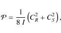
where CR2 and CS2 are the turbulent Reynolds stress and entropy contributions, respectively, and
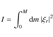
is the mode inertia,
where we have defined the ``source functions'':
where P is the gas pressure,
where
The kinetic spectrum E(k) is derived from the 3D simulation as detailled in Samadi et al. (2003b).
As shown by Samadi et al. (2003b), the k-dependence of Es(k) is
similar to that of the E(k). Accordingly, we assume
![]() .
.
In Samadi et al. (2008a), two different analytical functions for
![]() have been considered, namely a
Lorentzian function and a Gaussian one. In the present study we will
in addition derive
have been considered, namely a
Lorentzian function and a Gaussian one. In the present study we will
in addition derive
![]() directly from the 3D simulations
as detailled in Samadi et al. (2003a). Once
directly from the 3D simulations
as detailled in Samadi et al. (2003a). Once
![]() is derived
from the 3D simulation, it is implemented in Eqs. (5) and (6).
is derived
from the 3D simulation, it is implemented in Eqs. (5) and (6).
We compute the mode excitation as detailled in
Samadi et al. (2008a): all required quantities - except ![]() ,
I and
,
I and
![]() - are obtained directly from two 3D hydrodynamical simulations
representative of the outer layers of HD 49933, whose characteristics are described in
Sect. 2.2 below.
- are obtained directly from two 3D hydrodynamical simulations
representative of the outer layers of HD 49933, whose characteristics are described in
Sect. 2.2 below.
The quantities related to the modes (
![]() ,
I and
,
I and ![]() )
are calculated using the adiabatic pulsation code ADIPLS (Christensen-Dalsgaard & Berthomieu 1991) from 1D global models.
The outer layers of these 1D models are derived from the 3D
simulation as described in Sect. 2.3.
)
are calculated using the adiabatic pulsation code ADIPLS (Christensen-Dalsgaard & Berthomieu 1991) from 1D global models.
The outer layers of these 1D models are derived from the 3D
simulation as described in Sect. 2.3.
2.2 The 3D simulations
We computed two 3D radiation-hydrodynamical model atmospheres with the code
CO5BOLD (Wedemeyer et al. 2004; Freytag et al. 2002). One 3D simulation had a solar
iron-to-hydrogen [Fe/H] = 0.0 while the other had [Fe/H] = -1.0. The 3D model with
[Fe/H] = 0 (resp. [Fe/H] = -1) will be hereafter referred to as model S0 (resp. S1). The
assumed chemical composition is similar (in particular for the CNO elements)
to that of the solar chemical composition proposed by Asplund et al. (2005). The
abundances of the ![]() -elements in model S1 were assumed to be enhanced by
0.4 dex. For S0 we obtain
Z/X = 0.01830 and Y=0.249, and for S1
Z/X =
0.0036765 and Y=0.252. Both 3D simulations have exactly the same gravity
(
-elements in model S1 were assumed to be enhanced by
0.4 dex. For S0 we obtain
Z/X = 0.01830 and Y=0.249, and for S1
Z/X =
0.0036765 and Y=0.252. Both 3D simulations have exactly the same gravity
(
![]() )
and are very close in effective temperature (
)
and are very close in effective temperature (
![]() ).
Both models employ a spatial mesh with
).
Both models employ a spatial mesh with
![]() grid
points, and a physical extent of the computational box of
grid
points, and a physical extent of the computational box of
![]() Mm3. The equation of state takes into account the ionisation of
hydrogen and helium as well as the formation of H2 molecules according to
the Saha-Boltzmann statistics. The wavelength dependence of the radiative transfer
is treated by the opacity binning method (Nordlund 1982; Vögler et al. 2004; Ludwig 1992)
using five wavelength bins for model S0 and six for model S1. Detailed
wavelength-dependent opacities were obtained from the MARCS model
atmosphere package (Gustafsson et al. 2008). Table 1 summarizes the
characteristics of the 3D models. The effective temperature and surface
gravity correspond to the parameters of HD 49933 within the observational
uncertainties, while the two metallicities bracket the observed value.
Mm3. The equation of state takes into account the ionisation of
hydrogen and helium as well as the formation of H2 molecules according to
the Saha-Boltzmann statistics. The wavelength dependence of the radiative transfer
is treated by the opacity binning method (Nordlund 1982; Vögler et al. 2004; Ludwig 1992)
using five wavelength bins for model S0 and six for model S1. Detailed
wavelength-dependent opacities were obtained from the MARCS model
atmosphere package (Gustafsson et al. 2008). Table 1 summarizes the
characteristics of the 3D models. The effective temperature and surface
gravity correspond to the parameters of HD 49933 within the observational
uncertainties, while the two metallicities bracket the observed value.
For each 3D simulation, two time series were built. One has a long duration
(38h and 20h for S0 and S1, respectively) and a low sampling
frequency (10 mn). This time series is used to compute time averaged
quantities (
![]() ,
E(k), etc.). The second time series is shorter
(8.8 h and 6.8 h for S0 and S1, respectively), but has a high
sampling frequency (1 mn). Such high sampling frequency is required
for the calculation of
,
E(k), etc.). The second time series is shorter
(8.8 h and 6.8 h for S0 and S1, respectively), but has a high
sampling frequency (1 mn). Such high sampling frequency is required
for the calculation of
![]() .
Indeed, the modes we are looking at lie between
.
Indeed, the modes we are looking at lie between
![]() mHz and
mHz and
![]() mHz.
mHz.
Table 1: Characteristics of the 3D simulations.
The two 3D simulations extend up to
T=100 000 K. However, for
![]() K, the 3D simulations are not completely realistic. First of
all, the MARCS-based opacities are provided only up to a temperature of
30 000 K; for higher temperatures the value at 30 000 K is assumed. Note
that we refer to the opacity per unit mass here. For the radiative transfer
the opacity per unit volume is the relevant quantity, i.e. the product of
opacity per mass unit and density. Since in the simulation the opacity is
still multiplied at each position with the correct local density, the actual
error we make when extrapolating the opacity is acceptable.
K, the 3D simulations are not completely realistic. First of
all, the MARCS-based opacities are provided only up to a temperature of
30 000 K; for higher temperatures the value at 30 000 K is assumed. Note
that we refer to the opacity per unit mass here. For the radiative transfer
the opacity per unit volume is the relevant quantity, i.e. the product of
opacity per mass unit and density. Since in the simulation the opacity is
still multiplied at each position with the correct local density, the actual
error we make when extrapolating the opacity is acceptable.
Another limitation of the simulations is the restricted size of the computational box which does
not allow for a full development of the largest flow structures, again in the
layers above
![]() K. Two hints make us believe that the size
of the computational domain is not fully sufficient: i) in the deepest layers
of the simulations there is a tendency that structures align with the
computational grid; ii) the spatial spectral power P of scalar fields in a horizontal layer
does not tend towards the expected asymptotic behaviour
K. Two hints make us believe that the size
of the computational domain is not fully sufficient: i) in the deepest layers
of the simulations there is a tendency that structures align with the
computational grid; ii) the spatial spectral power P of scalar fields in a horizontal layer
does not tend towards the expected asymptotic behaviour
![]() for low
spatial wavenumber k. We noticed this shortcoming only after the completion of the simulation
runs. To mitigate its effect in our analysis, we will later by default integrate the
mode excitation rates up to
T = 30 000 K. However, for comparison purposes,
some computations have been extended down to the bottom of the 3D
simulations. For S0, the layers located below
for low
spatial wavenumber k. We noticed this shortcoming only after the completion of the simulation
runs. To mitigate its effect in our analysis, we will later by default integrate the
mode excitation rates up to
T = 30 000 K. However, for comparison purposes,
some computations have been extended down to the bottom of the 3D
simulations. For S0, the layers located below
![]() K contribute only by
K contribute only by ![]() 10% to the excitation of the modes lying in the frequency range where modes have the most chance to be detected (
10% to the excitation of the modes lying in the frequency range where modes have the most chance to be detected (
![]() mHz). For S1, the contribution of the deep layers
is even smaller (
mHz). For S1, the contribution of the deep layers
is even smaller (![]() 5%).
5%).
Finally, one may wonder how the treatment of the small-scales or the limited spatial resolution of the simulation can influence our calculations. Dissipative processes are handled in CO5BOLD on the one hand side implicitely by the numerical scheme (Roe-type approximate Riemann solver), and on the other hand explicitely by a sub-grid model according to the classical Smagorinsky (1963) formulation. Jacoutot et al. (2008) found that computed mode excitation rates significantly depend on the adopted sub-grid model. Samadi et al. (2007) have found that solar mode excitation rates computed in the manner of Nordlund & Stein (2001), i.e., using data directly from the 3D simulation, decrease as the spatial resolution of the solar 3D simulation decreases. As a conclusion the spatial resolution or the sub-grid model can influence computed mode excitation rates (see a discussion in Samadi et al. 2008a). However, concerning the spatial resolution and according to Samadi et al. (2007)'s results, the present spatial resolution (1/140 of the horizontal size of the box and about 1/150 of the vertical extent of the simulation box) is high enough to obtain accurate computed energy rates. The increased spatial resolution of our models in comparison to the work of Jacoutot et al. (2008) reduces the impact of the unresolved scales.
2.3 The 1D global models
For each 3D model we compute an associated 1D global model. The models are built in the manner of Trampedach (1997) as detailled in Samadi et al. (2008a) in such way that their outer layers are replaced by the averaged 3D simulations described in Sect. 2.2. The interior of the models are obtained with the CESAM code assuming standard physics: Convection is described according to Böhm-Vitense (1958)'s local mixing-length theory of convection (MLT), and turbulent pressure is ignored. Microscopic diffusion is not included. The OPAL equation of state is assumed. The chemical mixture of the heavy elements is similar to that of Asplund et al. (2005)'s mixture. As in Samadi et al. (2008a), we will refer to these models as ``patched'' models hereafter.
The two models have the effective temperature and the gravity of the
3D simulations. One model is matched with S0 and has [Fe/H] = 0, while the
second is matched with S1 and has [Fe/H] = -1. The 1D models have the
same chemical mixture as their associated 3D simulations.
The parameters of the 1D patched models are given in Table 2.
The stratification in density and temperature of the patched 1D models are shown in Fig. 1. At any given temperature the density is larger in S1 as a consequence of
its lower metal abundance. Indeed, the lower the metal abundance, the lower the opacity; then,
at a given optical depth (![]() ), the density is larger in S1 compared to S0.
The photosphere corresponds to the optical depth
), the density is larger in S1 compared to S0.
The photosphere corresponds to the optical depth
![]() .
Since
the two 3D simulations have approximatively the same effective
temperature, the density in S1 is larger at optical depth
.
Since
the two 3D simulations have approximatively the same effective
temperature, the density in S1 is larger at optical depth
![]() .
Since the density in S1 increases with depth even more rapidly than in S0, the density in S1 remains larger for
.
Since the density in S1 increases with depth even more rapidly than in S0, the density in S1 remains larger for
![]() than in S0.
than in S0.
Table 2:
Characteristics of the 1D ``patched'' models. ![]() is the
mixing-length parameter.
is the
mixing-length parameter.
![\begin{figure}
\par\includegraphics[width=9cm,clip]{11867fig1.eps}
\end{figure}](/articles/aa/full_html/2010/01/aa11867-09/img79.png)
|
Figure 1:
Mean density
|
| Open with DEXTER | |
3 Effects of the metal abundance on excitation rates
The mode excitation rates (![]() )
are computed for the two 3D simulations according
to Eqs. (1)-(6). The integration is performed from
the top of the simulated domains down to
T = 30 000 K (see Sect. 2.2).
In the following,
)
are computed for the two 3D simulations according
to Eqs. (1)-(6). The integration is performed from
the top of the simulated domains down to
T = 30 000 K (see Sect. 2.2).
In the following,
![]() (resp.
(resp.
![]() )
corresponds to the mode
excitation rates associated with the 3D model with [Fe/H] = -1 (resp. [Fe/H] = 0).
)
corresponds to the mode
excitation rates associated with the 3D model with [Fe/H] = -1 (resp. [Fe/H] = 0).
3.1 Results
Figure 2 shows the effect of the assumed metal abundance of the
stellar model on the mode excitation rates.
![]() is found to be three times smaller than
is found to be three times smaller than
![]() ,
i.e. p modes associated with the metal
poor 3D model (S1) receive approximatively three times less
energy per unit time than those associated with the 3D model with
the solar metal abundance (S0).
,
i.e. p modes associated with the metal
poor 3D model (S1) receive approximatively three times less
energy per unit time than those associated with the 3D model with
the solar metal abundance (S0).
For both 3D models, the dominant part of the
driving is ensured by the Reynolds stresses. The entropy fluctuations
contribute by only ![]() 30% of the total power for both S0 and S1. By comparison,
in the case of the Sun and
30% of the total power for both S0 and S1. By comparison,
in the case of the Sun and ![]() Cen A it contributes by only
Cen A it contributes by only ![]() 15%.
Furthermore, we find that the contribution of the entropy source term
is - as for the Reynolds stress term - about three times smaller in S1
than in S0. We conclude that the effect of the metal abundance
on the excitation rates is almost the same for the Reynolds stress
contribution and the entropy source term.
15%.
Furthermore, we find that the contribution of the entropy source term
is - as for the Reynolds stress term - about three times smaller in S1
than in S0. We conclude that the effect of the metal abundance
on the excitation rates is almost the same for the Reynolds stress
contribution and the entropy source term.
![\begin{figure}
\par\includegraphics[width=9cm,clip]{11867fig2.eps}
\end{figure}](/articles/aa/full_html/2010/01/aa11867-09/img82.png)
|
Figure 2:
Mode excitation rates
|
| Open with DEXTER | |
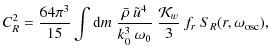
3.2 Interpretation
From Eqs. (1), (2), (3), (7)
and (8) we show that at a given layer the power supplied to the modes - per unit mass
- by the Reynolds stress is proportional to
![]() ,
where
,
where
![]() is the flux of the kinetic energy, which is
proportional to
is the flux of the kinetic energy, which is
proportional to
![]() ,
,
![]() is a characteristic length (see Sect. 2.1) and
is a characteristic length (see Sect. 2.1) and
![]() is the mode mass defined as:
is the mode mass defined as:

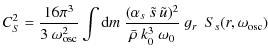
where
The power supplied to the modes - per unit mass -
by the entropy source term is proportional to
![]() where
where
![]() is the mode frequency,
is the mode frequency,
![]() ,
where
,
where
![]() is the convective flux, and finally
is the convective flux, and finally ![]() is the rms of the entropy fluctuations
(see Samadi et al. 2006). We recall that the higher
is the rms of the entropy fluctuations
(see Samadi et al. 2006). We recall that the higher
![]() ,
the higher the relative
contribution of the entropy source to the excitation.
We study below the role of
,
the higher the relative
contribution of the entropy source to the excitation.
We study below the role of ![]() ,
,
![]() ,
,
![]() ,
SR, Ss and
,
SR, Ss and ![]() :
:
- Mode mass (
 ):
The frequency domain, where modes are strongly excited, ranges between
):
The frequency domain, where modes are strongly excited, ranges between
 mHz and
 mHz. In this frequency domain, the
mode masses
associated with S0 are quite similar to those
associated with S1 (not shown). Consequently the differences between
mHz. In this frequency domain, the
mode masses
associated with S0 are quite similar to those
associated with S1 (not shown). Consequently the differences between
 and
and
 do not arise from the (small) differences in .
- Kinetic energy flux (
 ):
The larger
,
the larger the driving by the Reynolds stress.
However, we find that the two 3D models have very similar
.
This is not surprising since the two 3D models have very
similar effective temperatures. This means that the differences between
and
do not arise from the (small) differences in
.
):
The larger
,
the larger the driving by the Reynolds stress.
However, we find that the two 3D models have very similar
.
This is not surprising since the two 3D models have very
similar effective temperatures. This means that the differences between
and
do not arise from the (small) differences in
.
- Characteristic length (
 ):
In the manner of Samadi et al. (2003b) we derive from the
kinetic energy spectra E(k) of the two 3D
simulations the characteristic length
(
):
In the manner of Samadi et al. (2003b) we derive from the
kinetic energy spectra E(k) of the two 3D
simulations the characteristic length
(
 ,
see Eq. (8)) for each layer of the simulated domain.
We find that the differences in
between the two 3D simulations is small and does not play a
significant role in the differences in
,
see Eq. (8)) for each layer of the simulated domain.
We find that the differences in
between the two 3D simulations is small and does not play a
significant role in the differences in  .
This can be understood by the fact that S0 and S1 have the same
gravity. Indeed, as shown by Samadi et al. (2008a) - at a fixed
effective temperature -
scales as the inverse of g.
We conclude that the differences between
and
do not originate from the (small) differences in .
.
This can be understood by the fact that S0 and S1 have the same
gravity. Indeed, as shown by Samadi et al. (2008a) - at a fixed
effective temperature -
scales as the inverse of g.
We conclude that the differences between
and
do not originate from the (small) differences in .
- Source functions (SR and Ss):
The dimensionless source functions SR and Ss are
defined in Eqs. (5) and (6) respectively. Both source
functions involve the eddy time-correlation function
 .
We define
.
We define  as the frequency width of
.
As shown by Samadi et al. (2003a) and as verified in
the present case,
can be evaluated as the product k
uk where uk is given by the relation (Stein 1967):
as the frequency width of
.
As shown by Samadi et al. (2003a) and as verified in
the present case,
can be evaluated as the product k
uk where uk is given by the relation (Stein 1967):
where E(k) is normalised as:
According to Eqs. (10) and (11), uk is directly proportional to .
At a fixed k/k0, we then have
.
At a fixed k/k0, we then have
 .
.

We have plotted in Fig. 3 the characteristic velocity
![]() .
This quantity is found to be up to 15%
smaller for S1 compared with S0. In other words, the metal poor 3D
model is characterized by lower convective velocities. Consequently, the
source functions are smaller for S1 compared to S0.
Although the convective velocities differ between S0 and S1 by
only 15%, the excitation rates differ by a factor
.
This quantity is found to be up to 15%
smaller for S1 compared with S0. In other words, the metal poor 3D
model is characterized by lower convective velocities. Consequently, the
source functions are smaller for S1 compared to S0.
Although the convective velocities differ between S0 and S1 by
only 15%, the excitation rates differ by a factor ![]() 3.
The reason for this is that he source functions, which are non-linear functions
of
3.
The reason for this is that he source functions, which are non-linear functions
of
![]() ,
decrease very rapidly with
,
decrease very rapidly with
![]() .
This is
the consequence of the behavior of the eddy-time correlation
.
This is
the consequence of the behavior of the eddy-time correlation
![]() .
Indeed, this function varies with the ratio
.
Indeed, this function varies with the ratio
![]() approximately as a Lorentzian function.
This is why
approximately as a Lorentzian function.
This is why ![]() varies rapidly with
varies rapidly with
![]() (we
recall that
(we
recall that
![]() ).
).
In conclusion, the differences between
![]() and
and
![]() are mainly due to differences in the characteristic velocity
are mainly due to differences in the characteristic velocity
![]() .
In turn, the low convective velocity in S1 is a consequence of the
larger density compared to S0.
Indeed, as shown in Fig. 1, the density is systematically
higher in S1. At the layer where the modes are the most excited (i.e. at
.
In turn, the low convective velocity in S1 is a consequence of the
larger density compared to S0.
Indeed, as shown in Fig. 1, the density is systematically
higher in S1. At the layer where the modes are the most excited (i.e. at
![]() K), the density is
K), the density is ![]() 50% higher. Since the two 3D models have a similar kinetic energy flux (see
above), it follows that a larger density for S1 then implies lower
convective velocities.
50% higher. Since the two 3D models have a similar kinetic energy flux (see
above), it follows that a larger density for S1 then implies lower
convective velocities.
![\begin{figure}
\par\includegraphics[width=9cm,clip]{11867fig3.eps} \vspace*{4mm}
\end{figure}](/articles/aa/full_html/2010/01/aa11867-09/img111.png)
|
Figure 3:
Characteristic velocity
|
| Open with DEXTER | |
Relative contribution of the entropy source term (![]() ):
The convective flux
):
The convective flux
![]() in S1
is almost identical to that of S0. This is due to the fact that the
two 3D simulations have almost the same effective
temperature. Furthermore, as pointed out above, the differences in
in S1
is almost identical to that of S0. This is due to the fact that the
two 3D simulations have almost the same effective
temperature. Furthermore, as pointed out above, the differences in
![]() between S1 and S0 are small.
As a consequence, the ratio
between S1 and S0 are small.
As a consequence, the ratio
![]() does not differ between the two 3D simulations.
Accordingly, as for the Reynolds contribution, the variation of the excitation rates with the
metal abundance is only due to the source term SS. The latter
varies with
does not differ between the two 3D simulations.
Accordingly, as for the Reynolds contribution, the variation of the excitation rates with the
metal abundance is only due to the source term SS. The latter
varies with ![]() in the same manner as SR, which is in turn the reason for the contribution of the entropy fluctuations to show
the same trend with the metal abundance as the
Reynolds stress term.
in the same manner as SR, which is in turn the reason for the contribution of the entropy fluctuations to show
the same trend with the metal abundance as the
Reynolds stress term.
4 Theoretical calculation of
for HD 49933
We derive the mode excitation rates ![]() for HD 49933. According
to Gillon & Magain (2006), HD 49933 has
for HD 49933. According
to Gillon & Magain (2006), HD 49933 has
![]() dex, while
we only have two 3D simulations with values of [Fe/H], respectively
[Fe/H] = 0 and [Fe/H] = -1.
dex, while
we only have two 3D simulations with values of [Fe/H], respectively
[Fe/H] = 0 and [Fe/H] = -1.
As seen in Sect. 3.2, differences in ![]() between S0 and S1 are a direct consequence of the differences in the source functions SRand SS. It follows that in order to derive
between S0 and S1 are a direct consequence of the differences in the source functions SRand SS. It follows that in order to derive ![]() for HD 49933, we only have to
derive the expected values for SR and SS.
As seen in Sect. 3.2, differences in SR (or in
SS) between S0 and S1 are related to the surface metal
abundance through the surface densities that impact the convective velocities (
for HD 49933, we only have to
derive the expected values for SR and SS.
As seen in Sect. 3.2, differences in SR (or in
SS) between S0 and S1 are related to the surface metal
abundance through the surface densities that impact the convective velocities (![]() ).
The determination of the HD 49933 convective velocities allows us to determine its source
function. To this end, we use the fact that the kinetic flux is almost unchanged between
S1 and S0 (see Sect. 3.2) to derive the
profile of
).
The determination of the HD 49933 convective velocities allows us to determine its source
function. To this end, we use the fact that the kinetic flux is almost unchanged between
S1 and S0 (see Sect. 3.2) to derive the
profile of
![]() ,
expected at the
surface layers of HD 49933. This is performed by interpolating in Z between S0 and S1,
the surface density stratification representative of the surface layers of HD 49933.
The whole procedure is described in Appendix A.
,
expected at the
surface layers of HD 49933. This is performed by interpolating in Z between S0 and S1,
the surface density stratification representative of the surface layers of HD 49933.
The whole procedure is described in Appendix A.
In order to compute ![]() for HD 49933, we then need to know
Z for this star. Since we do not know its surface helium abundance, we will
assume by default the solar value for Y:
for HD 49933, we then need to know
Z for this star. Since we do not know its surface helium abundance, we will
assume by default the solar value for Y:
![]() (Basu 1997). Gillon & Magain (2006)'s analysis shows that the chemical
mixture of HD 49933 does not significantly differ from that of the
Sun. According to Asplund et al. (2005), the new solar metal to hydrogen ratio
is
(Basu 1997). Gillon & Magain (2006)'s analysis shows that the chemical
mixture of HD 49933 does not significantly differ from that of the
Sun. According to Asplund et al. (2005), the new solar metal to hydrogen ratio
is
![]() Accordingly, since [Fe/H] = -
Accordingly, since [Fe/H] = -
![]() dex, we derive
dex, we derive
![]() for HD 49933. Note that assuming Grevesse & Noels (1993)'s chemical mixture yields
for HD 49933. Note that assuming Grevesse & Noels (1993)'s chemical mixture yields
![]() .
.
The result of the calculation is shown in Fig. 2.
The maximum ![]() is
is
![]() J/s when Asplund et al. (2005)'s chemical composition is assumed (see
Appendix A). This is about 30 times larger than in the Sun and about 14 times
larger than in
J/s when Asplund et al. (2005)'s chemical composition is assumed (see
Appendix A). This is about 30 times larger than in the Sun and about 14 times
larger than in ![]() Cen A. When Grevesse & Noels (1993)'s chemical
mixture is assumed, the maximum in
Cen A. When Grevesse & Noels (1993)'s chemical
mixture is assumed, the maximum in
![]() is in that case equal to
is in that case equal to
![]() J/s, that is about 30% larger than with Asplund et al. (2005)'s solar chemical mixture.
J/s, that is about 30% larger than with Asplund et al. (2005)'s solar chemical mixture.
We note that the uncertainties in the knowledge of [Fe/H] set uncertainties on ![]() which
are on the order of 10% in the frequency domain of interest.
which
are on the order of 10% in the frequency domain of interest.
5 Conclusion
We have built two 3D hydrodynamical simulations representative in
effective temperature (
![]() )
and gravity (g) of the surface layers of an F type star on the main sequence. One model has a solar iron-to-hydrogen
abundance ([Fe/H] = 0) and the other has [Fe/H] = -1. Both models have the same
)
and gravity (g) of the surface layers of an F type star on the main sequence. One model has a solar iron-to-hydrogen
abundance ([Fe/H] = 0) and the other has [Fe/H] = -1. Both models have the same
![]() and g. For each 3D simulation, we have
computed an associated ``patched'' 1D full model.
Finally, we have computed the mode excitation rates
and g. For each 3D simulation, we have
computed an associated ``patched'' 1D full model.
Finally, we have computed the mode excitation rates ![]() associated
with the two ``patched'' 1D models.
associated
with the two ``patched'' 1D models.
Mode excitation rates associated with the metal poor 3D simulation are found to be about three times smaller than those associated with the 3D simulation which has a solar surface metal abundance. This is explained by the following connections: the lower the metallicity, the lower the opacity. At fixed effective temperature and surface gravity, the lower the opacity, the denser the medium at a given optical depth. The higher the density, the smaller are the convective velocities to transport the same amount of energy by convection. Finally, smaller convective velocities result in a less efficient driving. On the other hand, a surface metal abundance higher than the solar metal abundance will result in a lower surface density, which in turn will result in a higher convective velocity and then in a more efficient driving. Our result can then be qualitatively generalised for any surface metal abundance.
By taking into account the observed surface metal abundance of the star
HD 49933 (i.e. [Fe/H] = -0.37), we have derived, using two 3D
simulations and the interpolation procedure developed here, the rates
at which acoustic modes are expected to be excited by turbulent
convection in the case of
HD 49933. These excitation rates ![]() are found to be about two times
smaller than for a model built assuming a solar metal abundance.
These theoretical mode excitation rates will be used in Paper II
to derive the expected mode amplitudes from measured mode linewidths.
We will
then be able to compare these amplitudes with those derived for
HD 49933 from
different seismic data. This will constitute an indirect test of our
procedure which permits us to interpolate for any value of Z the mode excitation rates
are found to be about two times
smaller than for a model built assuming a solar metal abundance.
These theoretical mode excitation rates will be used in Paper II
to derive the expected mode amplitudes from measured mode linewidths.
We will
then be able to compare these amplitudes with those derived for
HD 49933 from
different seismic data. This will constitute an indirect test of our
procedure which permits us to interpolate for any value of Z the mode excitation rates ![]() between two 3D simulations with different Z but the same
between two 3D simulations with different Z but the same
![]() and
and ![]() .
We must stress that a more direct validation of this interpolation
procedure will be to compute a third 3D model with the surface metal
abundance of the star HD 49933 and to compare finally the mode
excitation rates obtained here with the interpolation procedure with
that obtained with this third 3D model.
This represents a long term work since several months (about three to
four months) are required for the calculation of this additional 3D
model, which is in progress.
.
We must stress that a more direct validation of this interpolation
procedure will be to compute a third 3D model with the surface metal
abundance of the star HD 49933 and to compare finally the mode
excitation rates obtained here with the interpolation procedure with
that obtained with this third 3D model.
This represents a long term work since several months (about three to
four months) are required for the calculation of this additional 3D
model, which is in progress.
We thank C. Catala for useful discussions concerning the spectrometric properties of HD 49933. We are indebted to J. Leibacher for his careful reading of the manuscript. K.B. acknowledged financial support from Liège University through the Subside Fédéral pour la Recherche 2009.
Appendix A: Theoretical calculation of the mode excitation rates for HD 49933
The mode excitation rate ![]() is inversely proportional to the mode
mass
is inversely proportional to the mode
mass ![]() (see Eqs. (9), (2) and (2)). This is why we can derive
(see Eqs. (9), (2) and (2)). This is why we can derive ![]() and
and
![]() separately in order to derive
separately in order to derive ![]() for HD 49933.
for HD 49933.
A.1 Derivation of

As pointed out in Sect. 3.2, the kinetic flux
![]() is almost unchanged between
S1 and S0 because both 3D models have the same
is almost unchanged between
S1 and S0 because both 3D models have the same
![]() .
This has also to be the case for HD 49933 (same
.
This has also to be the case for HD 49933 (same
![]() and
same
and
same ![]() than S0 and S1). Therefore, the
calculation of
than S0 and S1). Therefore, the
calculation of
![]() for HD 49933 relies only on the
evaluation of the values reached - at a fixed mode frequency - by the
source functions
for HD 49933 relies only on the
evaluation of the values reached - at a fixed mode frequency - by the
source functions
![]() and
and
![]() .
.
As seen in Sect. 3.2,
![]() controls the width of
controls the width of ![]() in a way that the source functions
in a way that the source functions
![]() and
and
![]() can be seen as functions of the
dimensionless ratio
can be seen as functions of the
dimensionless ratio
![]() .
The variation of E with k as well as the
variation of
.
The variation of E with k as well as the
variation of ![]() with
with
![]() are shown to be similar in
the two 3D simulations. Furthermore, S0 and S1 have approximately
the same characteristic length
are shown to be similar in
the two 3D simulations. Furthermore, S0 and S1 have approximately
the same characteristic length ![]() and hence approximately the same
and hence approximately the same
![]() .
Therefore, the source function
.
Therefore, the source function
![]() (resp.
(resp.
![]() )
associated with S0 only differs from that of S1
by the characteristic velocity
)
associated with S0 only differs from that of S1
by the characteristic velocity
![]() .
This must then also be the case for HD 49933.
Further, in order to evaluate the source functions in the case of HD
49933, we only need to know the factor
.
This must then also be the case for HD 49933.
Further, in order to evaluate the source functions in the case of HD
49933, we only need to know the factor ![]() by which
by which
![]() is modified in HD
49933 with respect to S1 or S0. According to Eq. (5)
(resp. Eq. (6)), multipling
is modified in HD
49933 with respect to S1 or S0. According to Eq. (5)
(resp. Eq. (6)), multipling
![]() by
by ![]() is
equivalent to replace
is
equivalent to replace
![]() (reps.
(reps.
![]() )
by
)
by
![]() (resp.
(resp.
![]() ).
).
Since the kinetic flux
![]() in HD 49933 must be the same for
S0 or S1, the characteristic velocity
in HD 49933 must be the same for
S0 or S1, the characteristic velocity
![]() can be derived for
HD 49933 according to
can be derived for
HD 49933 according to
![]() with
with
![]() where
where
![]() is the mean density stratification of S1,
is the mean density stratification of S1,
![]() the
characteritic velocity of S1 and
the
characteritic velocity of S1 and
![]() the mean density of
HD 49933. Once
the mean density of
HD 49933. Once ![]() and then
and then
![]() are derived for HD 49933, we then compute
the source functions associated with HD 49933.
Finally, we compute
are derived for HD 49933, we then compute
the source functions associated with HD 49933.
Finally, we compute
![]() by
keeping
by
keeping
![]() constant. We now turn to the derivation of the factor
constant. We now turn to the derivation of the factor ![]() .
.
A.2 Derivation of

To derive ![]() at a given T, we need to know
how the mean density
at a given T, we need to know
how the mean density
![]() varies with the metal abundance Z.
In order to this we consider five ``standard'' 1D models with five different values of
Z. These 1D models are built using the same physics as described in Sect. 2.3.
Two of these models have the same abundance as S0 and S1. All of the 1D models have approximately the same gravity (
varies with the metal abundance Z.
In order to this we consider five ``standard'' 1D models with five different values of
Z. These 1D models are built using the same physics as described in Sect. 2.3.
Two of these models have the same abundance as S0 and S1. All of the 1D models have approximately the same gravity (
![]() )
and the same effective temperature (
)
and the same effective temperature (
![]() K).
K).
The set of 1D models shows that - at any given temperature within the
excitation region -
![]() varies with Z rather linearly.
In order to derive
varies with Z rather linearly.
In order to derive
![]() for HD 49933, we apply - at fixed T and between S0 and S1 - a linear interpolation of
for HD 49933, we apply - at fixed T and between S0 and S1 - a linear interpolation of
![]() with respect to Z.
with respect to Z.
A.3 Derivation of
As shown in Sect. 3.2 above in the frequency domain where modes are
detected in HD 49933, ![]() does not change significantly
between S0 and S1. This suggests that the mode masses associated with
a patched 1D model with the metal abundance expected for HD 49933
would be very similar to those associated with S0 or S1.
Consequently we will assume for the case of HD 49933 the same mode masses
as those associated with S1, since this 3D model has a Z abundance
closer to that of HD 49933.
does not change significantly
between S0 and S1. This suggests that the mode masses associated with
a patched 1D model with the metal abundance expected for HD 49933
would be very similar to those associated with S0 or S1.
Consequently we will assume for the case of HD 49933 the same mode masses
as those associated with S1, since this 3D model has a Z abundance
closer to that of HD 49933.
A.4 Derivation of
Before deriving ![]() for HD 49933, we check that, from S0 and
the knowledge of
for HD 49933, we check that, from S0 and
the knowledge of
![]() ,
we can approximately reproduce
,
we can approximately reproduce
![]() ,
the mode excitation rates, associated with S1 following the procedure described above. Let
,
the mode excitation rates, associated with S1 following the procedure described above. Let
![]() .
As seen in Fig. 3, when we multiply
.
As seen in Fig. 3, when we multiply
![]() by
by
![]() we
matche
we
matche
![]() .
Then, using
.
Then, using
![]() and following the
procedure described above, we derive
and following the
procedure described above, we derive
![]() ,
the mode excitation rates
associated with S1 but derived from S0. The result is shown in Fig. A.1.
,
the mode excitation rates
associated with S1 but derived from S0. The result is shown in Fig. A.1.
![]() matches
matches
![]() rather well.
However, there are differences remaining in particular in the frequency domain
rather well.
However, there are differences remaining in particular in the frequency domain
![]() mHz. Nevertheless, the differences between
mHz. Nevertheless, the differences between
![]() and
and ![]() are
in any case not significant compared to the accuracy at which the mode
amplitudes are measured with the CoRoT data (see Paper II). This
validates the procedure, at least at the level of the current seismic
precisions.
are
in any case not significant compared to the accuracy at which the mode
amplitudes are measured with the CoRoT data (see Paper II). This
validates the procedure, at least at the level of the current seismic
precisions.
![\begin{figure}
\par\includegraphics[width=9cm,clip]{11867fig4.eps}
\vspace*{2mm}
\end{figure}](/articles/aa/full_html/2010/01/aa11867-09/img150.png)
|
Figure A.1:
Mode excitation rates
|
| Open with DEXTER | |
Since the metal abundance Z of HD 49933 is closer to that of S1 than that of S0, we
derive the mode excitation rates ![]() associated with
HD 49933 from S1 following the procedure detailled above.
The result is shown in Fig. 2.
As expected, the mode excitation rates
associated with
HD 49933 from S1 following the procedure detailled above.
The result is shown in Fig. 2.
As expected, the mode excitation rates ![]() associated with HD 49933 lie
between those ofS0 and S1, while remaining closer to S1 than to S0.
Note that the differences between
associated with HD 49933 lie
between those ofS0 and S1, while remaining closer to S1 than to S0.
Note that the differences between
![]() and the excitation
rates derived for HD 49933 (
and the excitation
rates derived for HD 49933 (![]() )
are of the same order as
the differences seen locally between
)
are of the same order as
the differences seen locally between
![]() and
and
![]() .
These differences remain small compared to the current seismic precisions.
On the other hand the differences between
.
These differences remain small compared to the current seismic precisions.
On the other hand the differences between ![]() and
and
![]() are significant and
have an important impact on the mode amplitudes (see Paper II).
are significant and
have an important impact on the mode amplitudes (see Paper II).
References
- Appourchaux, T., Michel, E., Auvergne, M., et al. 2008, A&A, 488, 705 [Google Scholar]
- Asplund, M., Grevesse, N., & Sauval, A. J. 2005, in Cosmic Abundances as Records of Stellar Evolution and Nucleosynthesis, ed. T. G. Barnes, III, & F. N. Bash, Conf. Ser., 336, 25 [Google Scholar]
- Basu, S. 1997, MNRAS, 288, 572 [NASA ADS] [Google Scholar]
- Belkacem, K., Samadi, R., Goupil, M. J., & Kupka, F. 2006a, A&A, 460, 173 [Google Scholar]
- Belkacem, K., Samadi, R., Goupil, M. J., Kupka, F., & Baudin, F. 2006b, A&A, 460, 183 [Google Scholar]
- Benomar, O., Baudin, F., Campante, T., et al. 2009, A&A, 507, L13 [Google Scholar]
- Böhm-Vitense, E. 1958, Z. Astrophys., 46, 108 [Google Scholar]
- Bruntt, H., De Cat, P., & Aerts, C. 2008, A&A, 478, 487 [Google Scholar]
- Chaplin, W. J., Houdek, G., Elsworth, Y., et al. 2005, MNRAS, 360, 859 [NASA ADS] [CrossRef] [Google Scholar]
- Christensen-Dalsgaard, J., & Berthomieu, G. 1991, Theory of solar oscillations, Solar interior and atmosphere, A92-36201 14-92 (Tucson: AZ university of Arizona Press), 401 [Google Scholar]
- Freytag, B., Steffen, M., & Dorch, B. 2002, Astron. Nachr., 323, 213 [NASA ADS] [CrossRef] [EDP Sciences] [Google Scholar]
- Gillon, M., & Magain, P. 2006, A&A, 448, 341 [Google Scholar]
- Grevesse, N., & Noels, A. 1993, in Origin and Evolution of the Elements, ed. N. Prantzos, E. Vangioni-Flam, & M. Cassé (Cambridge University Press), 15 [Google Scholar]
- Gustafsson, B., Edvardsson, B., Eriksson, K., et al. 2008, A&A, 486, 951 [Google Scholar]
- Houdek, G. 2006, in Proceedings of SOHO 18/GONG 2006/HELAS I, Beyond the spherical Sun, Published on CDROM, ESA SP, 624, 28.1 [Google Scholar]
- Houdek, G., Balmforth, N. J., Christensen-Dalsgaard, J., & Gough, D. O. 1999, A&A, 351, 582 [Google Scholar]
- Jacoutot, L., Kosovichev, A. G., Wray, A. A., & Mansour, N. N. 2008, ApJ, 682, 1386 [NASA ADS] [CrossRef] [Google Scholar]
- Ludwig, H.-G. 1992, Ph.D. Thesis, University of Kiel [Google Scholar]
- Mosser, B., Bouchy, F., Catala, C., et al. 2005, A&A, 431, L13 [Google Scholar]
- Neuforge-Verheecke, C., & Magain, P. 1997, A&A, 328, 261 [Google Scholar]
- Nordlund, A. 1982, A&A, 107, 1 [Google Scholar]
- Nordlund, Å., & Stein, R. F. 2001, ApJ, 546, 576 [Google Scholar]
- Samadi, R., & Goupil, M. . 2001, A&A, 370, 136 [Google Scholar]
- Samadi, R., Nordlund, Å., Stein, R. F., Goupil, M. J., & Roxburgh, I. 2003a, A&A, 404, 1129 [Google Scholar]
- Samadi, R., Nordlund, Å., Stein, R. F., Goupil, M. J., & Roxburgh, I. 2003b, A&A, 403, 303 [Google Scholar]
- Samadi, R., Kupka, F., Goupil, M. J., Lebreton, Y., & van't Veer-Menneret, C. 2006, A&A, 445, 233 [Google Scholar]
- Samadi, R., Georgobiani, D., Trampedach, R., et al. 2007, A&A, 463, 297 [Google Scholar]
- Samadi, R., Belkacem, K., Goupil, M. J., Dupret, M.-A., & Kupka, F. 2008a, A&A, 489, 291 [Google Scholar]
- Samadi, R., Belkacem, K., Goupil, M.-J., Ludwig, H.-G., & Dupret, M.-A. 2008b, Commun. Asteroseismol., 157, 130 [NASA ADS] [Google Scholar]
- Samadi, R., Ludwig, H., Belkacem, K., et al. 2010, A&A, 509, A16 (Paper II) [Google Scholar]
- Smagorinsky, J. 1963, Monthly Weather Rev., 91, 99 [Google Scholar]
- Solano, E., Catala, C., Garrido, R., et al. 2005, AJ, 129, 547 [NASA ADS] [CrossRef] [Google Scholar]
- Stein, R., Georgobiani, D., Trampedach, R., Ludwig, H.-G., & Nordlund, Å. 2004, Sol. Phys., 220, 229 [NASA ADS] [CrossRef] [Google Scholar]
- Stein, R. F. 1967, Sol. Phys., 2, 385 [NASA ADS] [CrossRef] [Google Scholar]
- Trampedach, R. 1997, Master's thesis, Aarhus University [Google Scholar]
- Vögler, A., Bruls, J. H. M. J., & Schüssler, M. 2004, A&A, 421, 741 [Google Scholar]
- Wedemeyer, S., Freytag, B., Steffen, M., Ludwig, H.-G., & Holweger, H. 2004, A&A, 414, 1121 [Google Scholar]
Footnotes
- ... CoRoT
- The CoRoT space mission, launched on December 27, 2006, has been developped and is operated by CNES, with the contribution of Austria, Belgium, Brasil, ESA, Germany and Spain.
All Tables
Table 1: Characteristics of the 3D simulations.
Table 2:
Characteristics of the 1D ``patched'' models. ![]() is the
mixing-length parameter.
is the
mixing-length parameter.
All Figures
|
|
Figure 1:
Mean density
|
| Open with DEXTER | |
| In the text | |
|
|
Figure 2:
Mode excitation rates
|
| Open with DEXTER | |
| In the text | |
|
|
Figure 3:
Characteristic velocity
|
| Open with DEXTER | |
| In the text | |
|
|
Figure A.1:
Mode excitation rates
|
| Open with DEXTER | |
| In the text | |
Copyright ESO 2010
Current usage metrics show cumulative count of Article Views (full-text article views including HTML views, PDF and ePub downloads, according to the available data) and Abstracts Views on Vision4Press platform.
Data correspond to usage on the plateform after 2015. The current usage metrics is available 48-96 hours after online publication and is updated daily on week days.
Initial download of the metrics may take a while.