| Issue |
A&A
Volume 509, January 2010
|
|
|---|---|---|
| Article Number | A96 | |
| Number of page(s) | 15 | |
| Section | Interstellar and circumstellar matter | |
| DOI | https://doi.org/10.1051/0004-6361/200911772 | |
| Published online | 22 January 2010 | |
The gravitational collapse of Plummer protostellar clouds
G. Arreaga-García1 - J. Klapp-Escribano2 - F. Gómez-Ramírez2,3
1 - Centro de
Investigación en Física, Universidad de Sonora, Blvd. Rosales
y Blvd. Encinas s/n Col. Centro, Hermosillo 83000, Sonora, Mexico
2 -
Instituto Nacional de
Investigaciones Nucleares, Carretera Mexico-Toluca s/n,
La Marquesa, Ocoyoacac 52750, Estado de Mexico, Mexico
3 -
Facultad de Ciencias,
Universidad Autónoma del Estado de Mexico, El Cerrillo Piedras
Blancas 50200, Estado de Mexico, Mexico
Received 2 February 2009 / Accepted 22 October 2009
Abstract
The growing observational evidence that main-sequence and
pre-main-sequence protostars are found in binary and multiple
systems suggests that they are formed by a fragmentation of
collapsing molecular cloud cores. In this paper we present the
results of a set of numerical simulations aimed to study the
gravitational collapse and fragmentation of a centrally condensed
cloud with a nearly flat central density region and a surrounding
gas envelope. In order to describe this cloud structure, we use the
Plummer radial density profile which satisfies the observed fact
that protostellar clouds have a flat central density profile in
their innermost region. We consider the cloud to be made of
molecular hydrogen and describe the thermodynamics with a single
barotropic equation of state, which includes a critical density
![]() as a unique free parameter that determines a
thermodynamical change on the collapsing gas: from an isothermal to
an adiabatic regime. In this paper we consider four different values
for the initial radius
as a unique free parameter that determines a
thermodynamical change on the collapsing gas: from an isothermal to
an adiabatic regime. In this paper we consider four different values
for the initial radius ![]() of the cloud, ranging from 2675 to
of the cloud, ranging from 2675 to
![]() .
In the models, for each ratio
.
In the models, for each ratio
![]() of the cloud
to core radius, we use two critical density values:
of the cloud
to core radius, we use two critical density values:
![]() and
and
![]() .
When the adiabatic change regime starts earlier, we find
interesting gas structures as a result of the collapse, although
these structures are different according to the initial mass content
of the envelope and the initial angular velocity of the cloud. When
the thermodynamical change occurs later, i.e., for
.
When the adiabatic change regime starts earlier, we find
interesting gas structures as a result of the collapse, although
these structures are different according to the initial mass content
of the envelope and the initial angular velocity of the cloud. When
the thermodynamical change occurs later, i.e., for
![]() ,
we observe that the
previously found structure is almost erased to give place instead to
a single clump of gas without any adorning spiral arms. In general,
we find that as the extension of the envelope mass increases, the
possibility of a model to produce a multiple system decreases. This
is a result of the initial configuration of our models, namely that
with bigger envelopes their cores have a lower ratio of rotational
to gravitational energy
,
we observe that the
previously found structure is almost erased to give place instead to
a single clump of gas without any adorning spiral arms. In general,
we find that as the extension of the envelope mass increases, the
possibility of a model to produce a multiple system decreases. This
is a result of the initial configuration of our models, namely that
with bigger envelopes their cores have a lower ratio of rotational
to gravitational energy ![]() ,
a lower ratio of thermal plus
rotational to gravitational energy
,
a lower ratio of thermal plus
rotational to gravitational energy
![]() ,
and a lower
angular velocity
,
and a lower
angular velocity ![]() ,
which induces a stronger collapse which
in turn contributes to the destruction of the structure that is
formed during the initial phases of the collapse. Thus in a
sufficient quantity rotational energy is crucial for the
fragmentation to occur and survive.
,
which induces a stronger collapse which
in turn contributes to the destruction of the structure that is
formed during the initial phases of the collapse. Thus in a
sufficient quantity rotational energy is crucial for the
fragmentation to occur and survive.
Key words: stars: formation - stars: low-mass
1 Introduction
The star formation process that occurs in the interstellar medium
begins when a prestellar molecular hydrogen cloud becomes
gravitationally bound. This earliest stage of cloud evolution lasts
![]() 106 years and is completed when a new star system is born
within the cloud.
106 years and is completed when a new star system is born
within the cloud.
In the central region of the system, a dense core is formed as the prestellar cloud collapses under its own self-gravity. The system is then composed of the central condensed core, usually named the protostellar core, and its surrounding gas envelope.
This protostellar phase is characterized by a high accretion rate
onto the protostellar core, so that about ![]() of the original
mass located in the surrounding gas envelope falls into the core in
about 104 years. Eventually, when most of the gas envelope has
been accreted or dissipated, the accretion rate becomes
significantly lower than in the protostellar stage.
of the original
mass located in the surrounding gas envelope falls into the core in
about 104 years. Eventually, when most of the gas envelope has
been accreted or dissipated, the accretion rate becomes
significantly lower than in the protostellar stage.
There are uncertainties in the evolution timescale of the cloud because it is obtained from statistical arguments. Despite this, any satisfactory star formation theory must reproduce at least the occurrence of these two stages of evolution, namely the prestellar and protostellar stages, see Ward-Thompson (2002).
We are interested in calculating the dynamical evolution of a cloud with the characteristics described above, although we begin in the protostellar stage without any concerns about the detailed process that the cloud has follow to reach such a stage. What matters most to us is to follow the gravitational collapse in the successful mathematical model of the observed structure of protostellar clouds.
Submillimeter dust emission and near-infrared absorption
observations of background stars suggest the mass structure of
protostellar clouds is strongly centrally condensed, with a nearly
constant central density value of ![]()
![]() in their innermost region (ranging from a few
to
in their innermost region (ranging from a few
to
![]() ). For the outer region, the protostellar surrounding
gas envelope has a density profile that falls with the radius as
). For the outer region, the protostellar surrounding
gas envelope has a density profile that falls with the radius as ![]() ,
with
,
with ![]() a constant, see André et al. (2004); Myers (2005).
a constant, see André et al. (2004); Myers (2005).
Recently Whitworth & Ward-Thompson (2001) proposed an empirical model to describe
an isolated and static protostellar cloud with a radial density
profile given by the Plummer (1911) function. Based on observational
lifetimes, these authors constrained the value of the exponent ![]() to be no more than
to be no more than ![]() .
Then they computed analytically
the subsequent evolution of the protostellar cloud with the
assumption that the gas has negligible pressure and rotation. They
concluded that this Plummer model captures some of the observed
behavior of the protostellar clouds. For instance, by comparing it
to the specific case of the observed L1544 dense core,
Tafalla et al. (1998) claimed the Plummer model to fit the observed
lifetime and accretion rate well.
.
Then they computed analytically
the subsequent evolution of the protostellar cloud with the
assumption that the gas has negligible pressure and rotation. They
concluded that this Plummer model captures some of the observed
behavior of the protostellar clouds. For instance, by comparing it
to the specific case of the observed L1544 dense core,
Tafalla et al. (1998) claimed the Plummer model to fit the observed
lifetime and accretion rate well.
The Plummer radial density function includes three free parameters:
![]() ,
establishing the central density value at the onset of the
protostellar cloud collapse; a critical radius R0 that sets up the
end of the approximately constant part of the radial density curve
for the innermost matter (
,
establishing the central density value at the onset of the
protostellar cloud collapse; a critical radius R0 that sets up the
end of the approximately constant part of the radial density curve
for the innermost matter (
![]() ); and an exponent
); and an exponent ![]() that fixes the density fall rate for a large radius (
that fixes the density fall rate for a large radius (![]() ).
).
In Arreaga-García et al. (2007,2008) we have furthermore studied the evolution of two types of models according to their initial radial density profile, which is either uniform or Gaussian. The uniform density model has been studied by many groups worldwide using different codes based on grids or particles, see for instance Bodenheimer et al. (2000) and references therein. As we successfully reproduced the uniform model results with a particle-based code, we established the reliability of our calculations. This was important because the Gaussian cloud model has been less studied with particle-based codes than the uniform model, despite the fact that the Gaussian model takes into account the observed property of protostellar clouds, which is that they are strongly centrally condensed.
For the reasons given above, we study in this paper the gravitational collapse of protostellar clouds with the Plummer radial density profile, as proposed by Whitworth & Ward-Thompson (2001). The models include rotation and pressure as in Arreaga-García et al. (2007,2008).
We will discuss the outcome of the simulations as we change the extension of the gas envelope surrounding the constant part of the Plummer radial density profile as well as the critical density value, after which the collapse changes from isothermal to adiabatic, see Sect. 2.2.
As Arreaga-García et al. (2007,2008), we use here the fully
parallelized Gadget2 code, which implements the Smoothed Particle
Hydrodynamics (![]() )
technique for solving the hydrodynamic
equations coupled to self-gravity. Once gravity has produced a
substantial contraction of the protostellar cloud, the gas begins to
heat. In order to take this increase of temperature into account, we
use a barotropic equation of state, as was proposed by
Boss et al. (2000), to model the thermodynamics of the gas.
)
technique for solving the hydrodynamic
equations coupled to self-gravity. Once gravity has produced a
substantial contraction of the protostellar cloud, the gas begins to
heat. In order to take this increase of temperature into account, we
use a barotropic equation of state, as was proposed by
Boss et al. (2000), to model the thermodynamics of the gas.
The outline of the paper is as follows. In Sect. 2
we describe the initial particle distribution of the simulations:
radial density profile, mass perturbation and the energy ratios ![]() and
and ![]() .
We give the values chosen for some of the
Gadget2 parameters. In Sect. 3 the simulations
are presented, including the physical properties of the resulting
protostellar cores. In Sect. 4 we discuss the
relevance of our simulations in view of reports elsewhere, and
finally we make some concluding remarks.
.
We give the values chosen for some of the
Gadget2 parameters. In Sect. 3 the simulations
are presented, including the physical properties of the resulting
protostellar cores. In Sect. 4 we discuss the
relevance of our simulations in view of reports elsewhere, and
finally we make some concluding remarks.
2 Initial conditions and computational considerations
2.1 Initial density profile
In Eq. (1) we show the mathematical function in which we are interested. It describes the observed fact that protostellar clouds have a flat central density profile in their innermost region. It was first introduced by Plummer (1911) and later on studied by Whitworth & Ward-Thompson (2001) in the context of the star formation theory. It reads as follows:
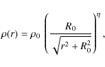
where
In order to apply the Plummer density function to model the specific
case of the observed L1544 protostellar dense core,
Whitworth & Ward-Thompson (2001) fixed the free parameters to the following
values:
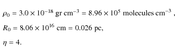
The mass contained in this core is
We have accomplished to have a set of 10 million ![]() particles
for all our simulations represent the initial configuration of the
protostellar cloud model. For instance, in Fig. 1 we
show the initial density profile as it is numerically measured for
different cloud radii
particles
for all our simulations represent the initial configuration of the
protostellar cloud model. For instance, in Fig. 1 we
show the initial density profile as it is numerically measured for
different cloud radii ![]() for the four initial configurations IC0,
IC1, IC2 and IC3, see Sect. 2.5 for more details of the initial
configurations and models. The average density
for the four initial configurations IC0,
IC1, IC2 and IC3, see Sect. 2.5 for more details of the initial
configurations and models. The average density
![]() for each
initial configuration is shown in Table 1 and in Fig. 2 we plot the total mass contained in the
protostellar cloud as a function of the radius r, as it is
obtained by direct integration of the Plummer function.
for each
initial configuration is shown in Table 1 and in Fig. 2 we plot the total mass contained in the
protostellar cloud as a function of the radius r, as it is
obtained by direct integration of the Plummer function.
Table 1: Parameters of the collapse models and outcome of the simulations.
![\begin{figure}
\par\includegraphics[width=7cm,clip]{11772f1.eps}\par\includegraphics[width=7cm,clip]{11772f1z.eps}
\end{figure}](/articles/aa/full_html/2010/01/aa11772-09/img179.png)
|
Figure 1:
Initial radial density profile for the initial
configurations |
| Open with DEXTER | |
![\begin{figure}
\par\includegraphics[width=6cm,clip]{11772f2.eps}
\end{figure}](/articles/aa/full_html/2010/01/aa11772-09/img180.png)
|
Figure 2:
Mass contained in a Plummer protostellar cloud as a
function of the radius. We calculate the mass from direct
integration of the Plummer function (solid line) and by counting the
|
| Open with DEXTER | |
2.2 Equation of state
According to astronomical observations, the regions from which stars
are formed consist basically of molecular hydrogen clouds at a
temperature of ![]()
![]() .
Therefore, the ideal equation of state
is a good approximation to account for the thermodynamics of the gas
in these clouds. However, once gravity has produced a substantial
contraction of the cloud, the opacity increases, the collapse
changes from isothermal to adiabatic and the gas begins to heat. To
include this increase in temperature into our calculations, we use
the barotropic equation of state proposed by Boss et al. (2000).
.
Therefore, the ideal equation of state
is a good approximation to account for the thermodynamics of the gas
in these clouds. However, once gravity has produced a substantial
contraction of the cloud, the opacity increases, the collapse
changes from isothermal to adiabatic and the gas begins to heat. To
include this increase in temperature into our calculations, we use
the barotropic equation of state proposed by Boss et al. (2000).
In order to correctly describe the non-isothermal regime, one needs
to solve the radiative transfer problem coupled to the hydrodynamic
equations, including a fully self-consistent energy equation to
obtain a precise knowledge of the dependence of temperature on
density. The implementation of radiative transfer has already been
included in some mesh-based codes. In ![]() ,
the incorporation of
radiative transfer has in general not been very satisfactory,
perhaps with the exception of Whitehouse & Bate (2006), in which they used
the flux-limited diffusion approximation to model the collapse of
molecular cloud cores. These authors suggested that there are
important differences in the temperature evolution of the cloud when
radiative transfer is properly taken into account.
,
the incorporation of
radiative transfer has in general not been very satisfactory,
perhaps with the exception of Whitehouse & Bate (2006), in which they used
the flux-limited diffusion approximation to model the collapse of
molecular cloud cores. These authors suggested that there are
important differences in the temperature evolution of the cloud when
radiative transfer is properly taken into account.
However, after comparing the results of our simulations in
Arreaga-García et al. (2007,2008) with those of Whitehouse & Bate (2006) for
the uniform density cloud, we concluded that the barotropic equation
of state in general behaves quite well and that we can capture the
essential dynamical behavior of the collapse. The simulations in
this paper are consequently carried out using the following
barotropic equation of state:
![\begin{displaymath}p= c_0^2 \rho \left[ 1 + \left(
\frac{\rho}{\rho_{\rm crit}}\right)^{\gamma -1 } \right] ,
\end{displaymath}](/articles/aa/full_html/2010/01/aa11772-09/img182.png)
where
In order to study the effect of changing the critical density, we
consider the following two values:
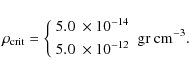
The critical density values
The isothermal evolution of a gravitationally collapsing cloud was
studied by Masunaga & Inutsuka (1999) for determining the critical
density at which the isothermal evolution is terminated. They
classified the condition for which isothermality is broken down into
three cases, i.e., when (1) the compressional heating rate overtakes
the thermal colling rate; (2) the optical depth for thermal
radiation reaches unity; and (3) the compressional heating rate
becomes comparable with the radiative diffusion energy transport
rate. The values obtained by Masunaga & Inutsuka (1999) depend
upon the temperature and opacity of the gas during the isothermal
regime and the density structure of the collapsing cloud for which
they used the Larson (1969) and Penston (1969) spherical isothermal
similarity solution. Despite the differences between Masunaga &
Inutsuka (1999) and this calculation, for example in the assumed
density structure of the collapsing cloud, there is a good
agreement in general with the
![]() values we have
selected, see their Sect. 2 and Fig. 1.
values we have
selected, see their Sect. 2 and Fig. 1.
As shown in Table 1, for models A0, A1, A2 and A3
![]() ,
while for
models B0, B1, B2 and B3
,
while for
models B0, B1, B2 and B3
![]() ,
see Sect. 2.5 for details of the initial
configurations and models.
,
see Sect. 2.5 for details of the initial
configurations and models.
We would like to ensure the correctness of our collapse results for
the Plummer cloud in this barotropic approximation by means of
comparing it with a model where all the thermal physics have been
accounted for. But as far as we know, the collapse of a centrally
condensed cloud with all the radiation physics included has not been
calculated. Therefore, we have to content ourselves at this time
with the extrapolation assumed in this paper, which is that the
barotropic equation of state is as good an approximation for
centrally condensed clouds as it was for the uniform density case.
Apart from the intrinsic difficulty of including in ![]() a proper
radiation transport treatment, there is the additional problem that
the calculations become prohibitively expensive from the
computational point of view.
a proper
radiation transport treatment, there is the additional problem that
the calculations become prohibitively expensive from the
computational point of view.
2.3 Initial energies
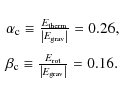
For all the initial configurations and models (see Sect. 2.5), the
particle distribution is constructed in a way that the cloud has the
same ratio of thermal and rotational energy with respect to the
gravitational energy, denoted by
![]() and
and
![]() ,
respectively. We have chosen the initial sound speed c0 and the
initial angular velocity
,
respectively. We have chosen the initial sound speed c0 and the
initial angular velocity
![]() of the cloud (see Table 1) in such a way that the cloud's energy ratios have
the following numerical values:
of the cloud (see Table 1) in such a way that the cloud's energy ratios have
the following numerical values:
These
On the other hand, observations (Goodman et al. 1993) have shown that
dense cores have velocity gradients of about 0.3 to
![]() ,
which translates into
,
which translates into
![]() to
to ![]()
![]() ,
which
is slightly below our value.
,
which
is slightly below our value.
The observational angular momentum - radius relation in molecular
cores has been reported by Goodman et al. (1993), see their Fig. 13.
Indeed, this plot has been reproduced and improved by Bodenheimer
(1995) in his Fig. 1. According to these plots, for our model A3
with
![]() its associated angular momentum is
its associated angular momentum is
![]() ,
which translate into angular
velocity becomes
,
which translate into angular
velocity becomes
![]() ,
which is very
close to our model A3 value.
,
which is very
close to our model A3 value.
Hence, our angular velocity range is in the happy mean of the one used by other authors in numerical calculations and suggested by observations.
2.4 Initial velocities and mass perturbations
For all models in this paper the initial protostellar cloud is in
counterclockwise rigid body rotation around the z axis; therefore
the initial velocity for the ith ![]() particle is given by
particle is given by
| (6) |
where the magnitude of the angular velocity
The initial density perturbation is applied to the mass of each
![]() simulation particle mi regardless of the cloud model
according to:
simulation particle mi regardless of the cloud model
according to:
where m0 is the unperturbed mass of the
2.5 The initial models
The initial structure of the cloud is constructed with the chosen
![]() and
and
![]() values as given in Sect. 2.3. The
assumed Plummer density profile depends upon the values selected for
the three model parameters, which are the central density
values as given in Sect. 2.3. The
assumed Plummer density profile depends upon the values selected for
the three model parameters, which are the central density
![]() ,
the radius
,
the radius
![]() and
the exponent
and
the exponent ![]() ,
see Eqs. (1) and (2). These three parameters
are the same for all models. We constructed four initial
configurations IC0, IC1, IC2 and IC3 with different envelopes that
extend to a cloud's radius
,
see Eqs. (1) and (2). These three parameters
are the same for all models. We constructed four initial
configurations IC0, IC1, IC2 and IC3 with different envelopes that
extend to a cloud's radius
![]() 0.5, 1.5, 2.5 and 3.7,
respectively. Each of the four basic initial configurations is split
into two depending on the
0.5, 1.5, 2.5 and 3.7,
respectively. Each of the four basic initial configurations is split
into two depending on the
![]() value. For the models
denoted by ``A'' (A0, A1, A2 and A3)
value. For the models
denoted by ``A'' (A0, A1, A2 and A3)
![]() ,
while for the ``B'' models (B0, B1, B2 and B3)
,
while for the ``B'' models (B0, B1, B2 and B3)
![]() .
For example, the
initial configuration IC1 is used for models A0 and B0, the only
difference is that the collapse of the B0 model changes later in the
evolution from isothermal to adiabatic.
.
For example, the
initial configuration IC1 is used for models A0 and B0, the only
difference is that the collapse of the B0 model changes later in the
evolution from isothermal to adiabatic.
As the radius and mass of the envelope increases, the lower density
of the outer region gets the average density to decrease from
![]() to
to
![]() for the initial configurations IC0 and IC3,
respectively, see Table 1. As the cloud's
for the initial configurations IC0 and IC3,
respectively, see Table 1. As the cloud's
![]() and
and
![]() values are the same for all initial configurations, their angular
velocity decreases from
values are the same for all initial configurations, their angular
velocity decreases from
![]() to
to
![]() for the initial configurations IC0 and IC3, respectively, see Table 1. The third column of Table 1, labeled with
for the initial configurations IC0 and IC3, respectively, see Table 1. The third column of Table 1, labeled with ![]() ,
is the total mass
contained in the cloud model.
,
is the total mass
contained in the cloud model.
The evolution and fragmentation of the cloud depends upon the global
![]() and
and
![]() ,
but also on the value of these two
quantities in the central high density region that first collapses.
Thus, the dynamical properties of the core are therefore of
fundamental importance for determining the fate of the whole cloud's
collapse.
,
but also on the value of these two
quantities in the central high density region that first collapses.
Thus, the dynamical properties of the core are therefore of
fundamental importance for determining the fate of the whole cloud's
collapse.
In our models, the cloud is composed of a core that extends to R0plus an envelope that extends to ![]() ,
see Table 1. For the initial
configuration IC0 there is no envelope and the cloud extends only to R0/2. The rotational and thermal energies must be shared somehow
between the core and the envelope when constructing the whole cloud.
To illustrate this energy sharing mechanism, we have calculated the
energy ratios for the core alone, neglecting particles whose
distance to the center of the cloud is greater than R0. The
results are presented in Table 2, where the
,
see Table 1. For the initial
configuration IC0 there is no envelope and the cloud extends only to R0/2. The rotational and thermal energies must be shared somehow
between the core and the envelope when constructing the whole cloud.
To illustrate this energy sharing mechanism, we have calculated the
energy ratios for the core alone, neglecting particles whose
distance to the center of the cloud is greater than R0. The
results are presented in Table 2, where the ![]() and
and ![]() values are calculated up to the core's radius R0.
values are calculated up to the core's radius R0.
![]() is
the initial angular velocity of the cloud.
is
the initial angular velocity of the cloud.
Table 2: Parameters of the collapse models for the initial configurations IC.
According to Table 2, the dynamical properties of the core for the initial configuration IC0 are, as expected, identical to the dynamical properties of the whole cloud.
Further important connections are that the bigger the envelope, the greater the thermal energy of the core while at the same time the rotational energy of the core is smaller. It is also interesting to note that for all models the sum of the energy ratios is always below 0.5 (the virial value), which means that the core has inherited the general tendency to collapse from the cloud.
The absolute value of the ratio of the hydrodynamic to the gravitational radial acceleration as a function of the radius for the four initial configurations IC0, IC1, IC2 and IC3 is presented in Fig. 3. The ratio is calculated by dividing the cloud into a number of spherical shells and averaging the radial accelerations within each shell. All initial configurations follow the same general trend, which is that near the center and surface of the cloud, the ratio reaches unity but is smaller than unity in most of the cloud. This indicates the tendency of the cloud to collapse, which is initiated in the whole cloud except very near the center and the surface. The ratio |ah/ag| tends to unity in the center because gravity becomes very weak and there is a balance between the force due to the pressure gradient and the gravity force. In the surface the ratio also reaches unity because of the uniform initial rotation assumed for the present models. Thus, the collapse of the surface follows the collapse of central regions of the cloud. A different surface behavior could be obtained with other choices for the initial rotation, for example differential, which is something we will explore in future communications.
![\begin{figure}
\par\includegraphics[width=9cm,clip]{11772f3.eps}
\end{figure}](/articles/aa/full_html/2010/01/aa11772-09/img217.png)
|
Figure 3: Absolute value of the ratio of the hydrodynamic to the gravitational radial acceleration as a function of the radius for the four initial configurations IC0, IC1, IC2 and IC3. |
| Open with DEXTER | |
2.6 Resolution
Following Truelove et al. (1997), the resolution requirement for avoiding
the growth of numerical instabilities is expressed in terms of the
Jeans wavelength
![]() ,
which is given by
,
which is given by

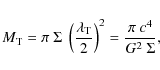
where G is Newton's universal gravitation constant, and c is the instantaneous sound speed. To obtain a more useful form for a particle based code, the Jeans wavelength
Nowadays it is well known that the Jeans requirement
Now, if we approximate the instantaneous sound speed by
![]() ,
then according to Eq. (3), we have that
,
then according to Eq. (3), we have that
![\begin{displaymath}M_{\rm J} = \frac{ \pi^{ \frac{5}{2} } }{6} \; \frac{c_0^3}{\...
...\rho_{\rm crit}
}\right)^{\gamma-1}\right]^{\frac{3}{2}} \cdot
\end{displaymath}](/articles/aa/full_html/2010/01/aa11772-09/img224.png)
Following Bate & Burkert (1997), the smallest mass that an
We define the mass of the simulation particles as
![]() ,
where
,
where ![]() is the total cloud's mass, and the total number of
particles
is the total cloud's mass, and the total number of
particles ![]() is 10 million for all the models in this paper.
is 10 million for all the models in this paper.
As in Arreaga-García et al. (2007,2008), because of the grid based
method of implementing our initial configuration of particles, the
mass of each ![]() particle is such that the given radial density
profile is satisfied. Despite this, we show below that for all
our simulations the resolution requirement stated by
Truelove et al. (1997) and Bate & Burkert (1997) is met very well.
particle is such that the given radial density
profile is satisfied. Despite this, we show below that for all
our simulations the resolution requirement stated by
Truelove et al. (1997) and Bate & Burkert (1997) is met very well.
As an example, let us consider model A0. We follow its collapse
until a peak density of
![]() .
For this model, from Table 1 its initial sound speed is
.
For this model, from Table 1 its initial sound speed is
![]() and from Eq. (10) its minimum Jeans mass is
given by
and from Eq. (10) its minimum Jeans mass is
given by
![]() ,
while we have
,
while we have
![]() .
Thus for model A0 we obtain the
ratio
.
Thus for model A0 we obtain the
ratio
![]() .
For model B0 the critical
density is
.
For model B0 the critical
density is
![]() and
the peak density is
and
the peak density is
![]() .
In this case we obtain
.
In this case we obtain
![]() for which the
mass ratio is
for which the
mass ratio is
![]() .
Although this ratio is
a factor of 10 greater than for model A0, the resolution
requirement for model B0 is also satisfied very easily.
.
Although this ratio is
a factor of 10 greater than for model A0, the resolution
requirement for model B0 is also satisfied very easily.
Additionally, it was demonstrated by Nelson (2006) that for
![]() simulations to accurately resolve the circumstellar disc, a
resolution criterion must be fulfilled as well. This criterion
establishes that for the vertical structure of the disc to be well
resolved, the scale-height H must be greater than four particle
smoothing lengths h at the disc mid-plane. As was the case for the
Jeans criterion, for an
simulations to accurately resolve the circumstellar disc, a
resolution criterion must be fulfilled as well. This criterion
establishes that for the vertical structure of the disc to be well
resolved, the scale-height H must be greater than four particle
smoothing lengths h at the disc mid-plane. As was the case for the
Jeans criterion, for an ![]() simulation this criterion is better
expressed in terms of mass rather than length; Nelson then defines
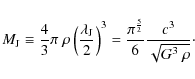
the Toomre mass, which is given by
simulation this criterion is better
expressed in terms of mass rather than length; Nelson then defines
the Toomre mass, which is given by
where
We can make a rough estimate of the Toomre mass for our simulations
by making use of the following approximation. Let us divide the disc
height H in slices of small ![]() .
We first calculate the
average volume density
.
We first calculate the
average volume density
![]() for every slice, then the
relation between surface and volume densities for every slice is
for every slice, then the
relation between surface and volume densities for every slice is
![]() .
If we consider that H for
most of our models is approximately given by
.
If we consider that H for
most of our models is approximately given by
![]() ,
where
,
where
![]() is the initial radius of the cloud, then the Toomre mass for
model A0 is given by
is the initial radius of the cloud, then the Toomre mass for
model A0 is given by
![]() .
.
Now, following Nelson (2006), the smallest mass resolution mnfor a simulation to prevent the appearance of numerically induced
fragmentation of the disc must be given by six times the average
number of the neighboring particles considered, therefore for our case
we have that
![]() .
On the other hand, as we have seen earlier,
the mass of the
.
On the other hand, as we have seen earlier,
the mass of the ![]() particle for our simulations is
particle for our simulations is
![]() ,
therefore the mass ratio which is
directly related to the resolution criterion is given by
,
therefore the mass ratio which is
directly related to the resolution criterion is given by
![]() .
Thus, our simulations also have enough mass
resolution in the disc.
.
Thus, our simulations also have enough mass
resolution in the disc.
2.7 Evolution code
We have carried out the time evolution of the initial particle
distribution with the Gadget2 parallel code, which is described in
detail by Springel (2005). Gadget2 is based on the tree-PMmethod for computing the gravitational forces and on the standard
![]() method for solving the hydrodynamic Euler equations.
method for solving the hydrodynamic Euler equations.
Gadget2 incorporates the following standard features: (i) each
particle i has its own smoothing length hi; (ii) the particles
are also allowed to have individual gravitational softening lengths
![]() ,
whose values are adjusted so that for every time step
,
whose values are adjusted so that for every time step
![]() is of order unity.
is of order unity.
Following Gabbasov et al. (2006), some empirical formulas are known to
assign a value to
![]() in order to minimize errors in the
calculation of the gravitational force on a particle i of the mass
mi. However, Gadget2 fixes the value of
in order to minimize errors in the
calculation of the gravitational force on a particle i of the mass
mi. However, Gadget2 fixes the value of
![]() for each
time-step using the minimum smoothing length value of all particles,
that is, if
for each
time-step using the minimum smoothing length value of all particles,
that is, if
![]() for i=1,2...N, then
for i=1,2...N, then
![]() .
.
The Gadget2 code that we have used in this paper has implemented a
Monaghan-Balsara form for the artificial viscosity,
see Monaghan & Gingold (1983) and Balsara (1995). The strength of the
viscosity is regulated by setting the parameter
![]() and
and
![]() ,
see Eq. (14) in Springel (2005).
We have fixed the Courant factor to 0.1. In order to move the
particles forward in time, Gadget2 uses a second order leapfrog algorithm.
,
see Eq. (14) in Springel (2005).
We have fixed the Courant factor to 0.1. In order to move the
particles forward in time, Gadget2 uses a second order leapfrog algorithm.
3 Results
For presenting the result of the simulations, we use iso-density
contour plots for a slice of particles around the equatorial plane
of the cloud. The bar located at the bottom of the plots shows the
![]() density range at a time t normalized with the initial
density
density range at a time t normalized with the initial
density ![]() .
A color scale is then associated with the value of
.
A color scale is then associated with the value of
![]() .
For instance, the color scale uses
yellow to indicate higher densities, blue for lower densities, and green
and orange for intermediate densities.
.
For instance, the color scale uses
yellow to indicate higher densities, blue for lower densities, and green
and orange for intermediate densities.
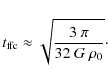
The free fall time
![]() sets a characteristic time scale for
the collapse of protostellar clouds which is given by
sets a characteristic time scale for
the collapse of protostellar clouds which is given by
|
(12) |
The free fall time scale
Due to the fact that the centrifugal force along the equator of the cloud is greater than at the poles, the contraction of the cloud is faster along the rotation axis, and the cloud evolves through a sequence of flat configurations.
The cloud decays in about one free fall time from a spherical to a flat configuration as most of the particles are contained in a narrow slice of matter around the equatorial plane. The accretion of particles takes place with cylindrical symmetry with respect to the rotation axis. During this first stage of gravitational contraction, the cloud reduces its dimensions to about 10% of its original size.
Later on, when the flattening of the cloud is extreme, the central part becomes slightly stretched taking the form of an oblate ellipsoid. As long as the cloud continues rotating, the central part will adopt a more elongated and slightly curved configuration, as was demonstrated by Burkert & Hartmann (2004).
The main results of the paper are summarized as follows.
3.1 Models A0 and B0: clouds with

The initial radius of these models is only
![]() ,
and the mass contained in the cloud
is
,
and the mass contained in the cloud
is
![]() ,
where M0 is the mass in the
protostellar core characterized by Eq. (2). Because of
their small size, these models have the highest initial average
density
,
where M0 is the mass in the
protostellar core characterized by Eq. (2). Because of
their small size, these models have the highest initial average
density
![]() ,
which
is of the same order of the central density as the Plummer density
function
,
which
is of the same order of the central density as the Plummer density
function ![]() ,
see Fig. 1. These models have the
highest angular velocity,
,
see Fig. 1. These models have the
highest angular velocity,
![]() .
.
The density fall with the radius is not significant, i.e., the end of
the cloud is reached too early for the fall of the density to be really
noticeable during the evolution. For this reason, we expect the
evolution of these models to be similar to the uniform density cloud
model for which
![]() ,
see
Arreaga-García et al. (2007,2008).
,
see
Arreaga-García et al. (2007,2008).
When the cloud has reached its maximum flattening, the ![]() particles with the highest density start forming an ellipsoidal
structure in the central region of the cloud.
particles with the highest density start forming an ellipsoidal
structure in the central region of the cloud.
Burkert & Hartmann (2004) demonstrated that as the structure collapses, it becomes
even more elongated and takes a bar-like shape with larger mass
concentrations at the end points, which are close to or outside the
foci of the initial elliptical structure. The cloud gives up some of
its initial angular momentum to this resulting bar-like structure,
which is large enough to prevent the total collapse of the bar. As
the density of the ![]() particles further increases, this bar-like
structure becomes a thin filament with two density maxima located at
the filament end points, as can be seen in panels c and d of Fig. 4. However, as time goes by, gas along the filament
starts to be pulled in by the focal point concentrations near the
ends of the filament.
particles further increases, this bar-like
structure becomes a thin filament with two density maxima located at
the filament end points, as can be seen in panels c and d of Fig. 4. However, as time goes by, gas along the filament
starts to be pulled in by the focal point concentrations near the
ends of the filament.
![\begin{figure}
\par\includegraphics[width=15cm]{11772f4.eps}
\end{figure}](/articles/aa/full_html/2010/01/aa11772-09/img279.png)
|
Figure 4:
Isodensity contours of the cloud mid-plane for model A0
with
|
| Open with DEXTER | |
![\begin{figure}
\par\includegraphics[width=15cm]{11772f5.eps}
\end{figure}](/articles/aa/full_html/2010/01/aa11772-09/img285.png)
|
Figure 5:
Isodensity contours of the cloud mid-plane for model B0
with
|
| Open with DEXTER | |
Shortly after, we note that these small cores become connected by a
very well defined bridge of particles; therefore for the two
models A0 and B0 a filament is formed connecting two matter
clumps,
regardless of the different critical density value
![]() of
each model. A binary system is formed which is clearly reminiscent
of the uniform density model studied in
Arreaga-García et al. (2007,2008). Up to this point, the evolution of
models A0 and B0 proceeds in an identical fashion.
of
each model. A binary system is formed which is clearly reminiscent
of the uniform density model studied in
Arreaga-García et al. (2007,2008). Up to this point, the evolution of
models A0 and B0 proceeds in an identical fashion.
The behavior of the filament of particles connecting the matter clumps is what makes the difference in the subsequent evolution: for model A0 the filament disappears, while for model B0 becomes thinner.
In model A0 the adiabatic regime enters earlier than in model B0, the collapse slows down earlier and due to gravity, the clumps become closer to one another along the filament, which finally disappears and the clumps merge to give place to a single protostellar fragment surrounded by spiral arms. However, the spiral arms start accumulating mass, where in addition to the central fragment, two exterior fragments appear resulting from the breakage of these spiral arms. Therefore, up to the dynamical time that we have been able to follow the evolution of this system, it is likely that it will end up with three fragments.
As was demonstrated by Burkert & Hartmann (2004), every flattening gas configuration will produce a bar-like structure that forms in the cloud's central region with clumps of matter developing at each bar-like end.
The rotation of the cloud only slows down the collapse, and the bar-like structure becomes a shrinking filament. Clumps of matter continue developing, but each time over a smaller length scale.
For model B0 the collapse continues all along the filament, as can be seen in Fig. 5. The two clumps that are formed in both models tend to virialize.
3.2 Models A1 and B1: clouds with

As can be noticed in Fig. 1, for these models the
initial density profile falls to ![]()
![]() .
For
this cloud the average initial density is
.
For
this cloud the average initial density is
![]() ,
the initial radius is
,
the initial radius is
![]() ,
and the initial angular velocity is
,
and the initial angular velocity is
![]() .
.
The fall of the density profile is more significant and the initial angular velocity is a factor of 3.2 smaller than for the models A0 and B0, and therefore we expect a different dynamical behavior.
In Fig. 6 we show the somehow complicated time history
of model A1 with a critical density
![]() .
After the cloud flattens along the
normal direction of the equatorial plane, a small bar is formed
surrounded by long spiral arms. Because the rotation speed of the
spiral arms and that of the bar are different, the spiral arms
become separated from the bar, giving place to the appearance of two
additional clumps of matter that move around the central bar.
Shortly after, the central clump loses its elongated form to become
cylindrical, while the two new clumps accumulate mass.
.
After the cloud flattens along the
normal direction of the equatorial plane, a small bar is formed
surrounded by long spiral arms. Because the rotation speed of the
spiral arms and that of the bar are different, the spiral arms
become separated from the bar, giving place to the appearance of two
additional clumps of matter that move around the central bar.
Shortly after, the central clump loses its elongated form to become
cylindrical, while the two new clumps accumulate mass.
The recently formed clumps as well as the older clump develop new spiral arms. A breakage of these new spiral arms occurs, giving place to the coexistence of up to four fragments as can be seen in the last panel of Fig. 6. Until the time that we were able to follow the evolution of this simulation, the quadruple system persisted with no further merging.
In Fig. 8 (left panel) we have followed the path of the centers when only three fragments are present for a short period of time. We also show in Fig. 8 (right panel) the path of the four fragments that appears after the occurrence of the second breakage of the spiral arms.
In model B1, with
![]() ,
the cloud experiences a stronger collapse resulting again
in a system with a central bar and spiral arms, but of a smaller size
than the system in model A1, as can now be seen in Fig. 7. In this case, there is no breakage of the spiral
arms from the central bar. There is a tendency of the central region
to fragment, retaining its spiral structure. The single resulting
system shows a general tendency to virialize.
,
the cloud experiences a stronger collapse resulting again
in a system with a central bar and spiral arms, but of a smaller size
than the system in model A1, as can now be seen in Fig. 7. In this case, there is no breakage of the spiral
arms from the central bar. There is a tendency of the central region
to fragment, retaining its spiral structure. The single resulting
system shows a general tendency to virialize.
![\begin{figure}
\par\includegraphics[width=15cm]{11772f6.eps}
\end{figure}](/articles/aa/full_html/2010/01/aa11772-09/img302.png)
|
Figure 6:
Isodensity contours of the cloud mid-plane for model A1
with
|
| Open with DEXTER | |
![\begin{figure}
\par\includegraphics[width=15cm]{11772f7.eps}
\end{figure}](/articles/aa/full_html/2010/01/aa11772-09/img309.png)
|
Figure 7:
Isodensity contours of the cloud mid-plane for model B1
with
|
| Open with DEXTER | |
![\begin{figure}
\par\includegraphics[width=6cm,clip]{11772f8a.eps}\hspace*{3mm}
\includegraphics[width=6cm,clip]{11772f8b.eps}
\end{figure}](/articles/aa/full_html/2010/01/aa11772-09/img310.png)
|
Figure 8: Centers for model A1. |
| Open with DEXTER | |
![\begin{figure}
\par\includegraphics[width=15cm]{11772f9.eps}
\end{figure}](/articles/aa/full_html/2010/01/aa11772-09/img321.png)
|
Figure 9:
Isodensity contours of the cloud mid-plane for model A2
with
|
| Open with DEXTER | |
![\begin{figure}
\par\includegraphics[width=13cm]{11772f10.eps}
\vspace*{4mm}
\end{figure}](/articles/aa/full_html/2010/01/aa11772-09/img326.png)
|
Figure 10:
Isodensity contours of the cloud mid-plane for model B2
with
|
| Open with DEXTER | |
![\begin{figure}
\par\includegraphics[width=15cm]{11772f11.eps}
\end{figure}](/articles/aa/full_html/2010/01/aa11772-09/img334.png)
|
Figure 11:
Isodensity contours of the cloud mid-plane for model A3
with
|
| Open with DEXTER | |
![\begin{figure}
\par\includegraphics[width=15cm]{11772f12.eps}
\end{figure}](/articles/aa/full_html/2010/01/aa11772-09/img342.png)
|
Figure 12:
Isodensity contours of the cloud mid-plane for model B3
with
|
| Open with DEXTER | |
3.3 Models A2 and B2: clouds with

In this case the initial radius of the cloud is
![]() ,
see Fig. 1. The
average initial density is
,
see Fig. 1. The
average initial density is
![]() and the initial angular velocity is
and the initial angular velocity is
![]() .
.
In model A2 a central well defined bar is formed, see Fig. 9. The surrounding spiral arms give a complete turn around the bar. Shortly after the bar decays into a single clump, we view the spirals as a ring circling the central clump. For this model we observe the formation of several fragments by means of the breakage of the spiral arms, although this phenomenon occurs in a more complicated way than in previous models. Although there is merging among fragments, it is very likely that this simulation ends up with a binary system, see Fig. 9. The central fragment is more massive than the surrounding fragments, and some of the fragments tend to virialize.
For model B2 we see a strong collapse towards a central clump, as can be seen in Fig. 10. There is a similarity between the results of models B1 and B2, which indicates that the value of the critical density is more determinant for the result of the simulations than their slight difference in the initial density profile and the initial angular velocity.
3.4 Models A3 and B3: clouds with

The initial radius of the cloud is
![]() ,
the average initial density is
,
the average initial density is
![]() ,
and the initial angular velocity is
,
and the initial angular velocity is
![]() .
These
.
These
![]() and
and
![]() values are the smallest of all models. The initial radial
density profile is shown in Fig. 1. In this case, the
difference in the density curves between the Gaussian and Plummer
functions is more notorious than in the previous models.
values are the smallest of all models. The initial radial
density profile is shown in Fig. 1. In this case, the
difference in the density curves between the Gaussian and Plummer
functions is more notorious than in the previous models.
In view of the outcome of the previous model B2, one would think that models A3 and B3 are not interesting, except for the fact that the central region of model A3 again shows a clear tendency to fragment towards a close binary system, as can be seen in Fig. 11.
For model B3 the collapse is so strong towards the center of the cloud that there is no indication of any fragmentation, as one can see in Fig. 12.
4 Discussion and concluding remarks
In order to explain the formation of binary stars, one of the mechanisms that has been proposed is prompt fragmentation, see Tohline (2002). The basic idea is that during the collapse of an isolated rotating molecular gas cloud, it may spontaneously break into two (or even more) fragments that enter into a stable orbit one around the other.
With the purpose of testing the prompt fragmentation mechanism, we present models of collapsing dense cores from centrally condensed initial states. These models are appropriate to be studied since starless cores in star-forming regions are in fact observed to be centrally condensed. The questions of how molecular clouds can reach such centrally condensed states and how the collapse is initiated are still open.
For the initially rigid rotation models presented in this paper, we have implemented a Plummer density profile with a linear mass perturbation scheme seeking to promote the generation of binary systems.
The evolution of the models studied in this work is determined
by two main factors, which are the initial structure of the cloud and
the value selected for the critical density
![]() above
which the collapse changes from isothermal to adiabatic.
above
which the collapse changes from isothermal to adiabatic.
The models we have presented show that as the size of the envelope
increases, the tendency to fragment decreases. This is a result of
the fact that as described in Sect. 2.5, for our models with
bigger envelopes, ![]() ,
,
![]() and
and ![]() are
lower, and the collapse that contributes to the destruction of the
structure which is formed during the initial phases of the collapse
is stronger. It is consequently crucial for any fragmentation to
occur that there is enough rotational energy.
are
lower, and the collapse that contributes to the destruction of the
structure which is formed during the initial phases of the collapse
is stronger. It is consequently crucial for any fragmentation to
occur that there is enough rotational energy.
In the case of our model A3, the rotational energy left to the core is insufficient for the collapsing core to develop any barlike structure (or S-shaped spiral pattern) in the central region. In this situation, the core can not fragment, as we have observed in our calculation.
The second factor that affects the evolution of the models studied
in this work is the value of the critical density
![]() for
a particular model. This paper showed that if the collapse changes
from isothermal to adiabatic earlier, which occurs for the models
with a lower critical density
for
a particular model. This paper showed that if the collapse changes
from isothermal to adiabatic earlier, which occurs for the models
with a lower critical density
![]() ,
the collapse is slowed
down more (but not completely stopped), and this gives the fragments
that are generated during the collapse the possibility to survive.
This can clearly be seen in Fig. 13 which shows the
time evolution of the maximum density in the cloud. For the
,
the collapse is slowed
down more (but not completely stopped), and this gives the fragments
that are generated during the collapse the possibility to survive.
This can clearly be seen in Fig. 13 which shows the
time evolution of the maximum density in the cloud. For the
![]() case, the collapse
is not slowed down very much even up to the point that the numerical
calculations are terminated, and this erased all the previously
formed structure. For the models with
case, the collapse
is not slowed down very much even up to the point that the numerical
calculations are terminated, and this erased all the previously
formed structure. For the models with
![]() ,
the collapse was significantly slowed down
and the structure survived. Consequently we can conclude that if the
collapse changes from isothermal to adiabatic early enough, the
survival probability of the fragments greatly increases.
,
the collapse was significantly slowed down
and the structure survived. Consequently we can conclude that if the
collapse changes from isothermal to adiabatic early enough, the
survival probability of the fragments greatly increases.
![\begin{figure}
\par\includegraphics[width=12cm,clip]{11772f13.eps}
\end{figure}](/articles/aa/full_html/2010/01/aa11772-09/img353.png)
|
Figure 13:
Evolution of the maximum density of the cloud for all
models. The time t is given in units of the free fall time
|
| Open with DEXTER | |
As described in Sect. 3.1, in model A0 we observed that the two formed clumps at the filament ends merge into one single central clump of matter. This merging event occurred as a consequence of both a loss in the clump's angular momentum and the gravitational interaction between clumps.
We emphasize that there are also simulations in which the closeness between clumps also occurred, but the final merge is avoided, see for example Arreaga-García et al. (2007), Bate et al. (1995) and references in which the standard isothermal test calculation was reproduced. For this test model, the two clumps pass each other instead of merging, and they finally enter into orbit around each other.
The cause behind this different behavior, which may decide whether or not a merging occurs, is perhaps the existence of small variations in the positions and velocities of the particles, which may come from the randomness of the initial particle distribution as discussed below.
The density perturbation in Eq. (7) plays a very important role in the merging issue. Indeed, the mass perturbation will cause the development of the two small regions where the mass of the cloud will be first accreted. Once the cloud has acquired a flattened configuration, the higher density gas will form an elliptical structure with these small accretion regions as focal points. As was demonstrated by Burkert & Hartmann (2004), the fate of this elliptical structure is always to collapse into a filament with a strong accumulation of mass at each end point.
As we have implemented a symmetric mass perturbation with respect to the origin of the coordinates of the cloud's equatorial plane, the clumps that will form will be antipodes of each other in such a way that an imaginary line joining them will pass through the coordinate of origin too.
Every clump exerts a gravitational torque on the other clump. Then
the velocity of the particles in the clumps begins to align with the
imaginary axis of symmetry joining the clumps, that is,
![]() ,
with the net effect that these particles lose
angular momentum. It follows that the particles which are accreted
into the clumps are those with the lower angular momentum, whereas
those accreted into the surrounding spiral arms are those with the
higher angular momentum. As the clumps lose their angular momentum,
the gravity force which every clump exerts on the other makes them
become closer to each other until they finally merge.
,
with the net effect that these particles lose
angular momentum. It follows that the particles which are accreted
into the clumps are those with the lower angular momentum, whereas
those accreted into the surrounding spiral arms are those with the
higher angular momentum. As the clumps lose their angular momentum,
the gravity force which every clump exerts on the other makes them
become closer to each other until they finally merge.
It is well known that when the gas gets a flattened configuration,
it is susceptible to fragmentation, for instance, all clouds with
![]() are expected to fragment. As
far as we know, it is not yet totally clear under which physical
conditions these dense cores form, become unstable and so trigger
the gravitational collapse, or why all the mechanisms for
fragmentation occur. This issue is as yet unclear because the
parameter space of the initial conditions is very large, and there
are many possibilities for the constitutive physics. Besides,
several disturbing environmental effects could also be present which
may affect the fate of the collapse, as discussed by
Goodwin et al. (2007). However, it appears that the main mechanism for the
formation of multiple systems is the fragmentation of circumstellar
discs.
are expected to fragment. As
far as we know, it is not yet totally clear under which physical
conditions these dense cores form, become unstable and so trigger
the gravitational collapse, or why all the mechanisms for
fragmentation occur. This issue is as yet unclear because the
parameter space of the initial conditions is very large, and there
are many possibilities for the constitutive physics. Besides,
several disturbing environmental effects could also be present which
may affect the fate of the collapse, as discussed by
Goodwin et al. (2007). However, it appears that the main mechanism for the
formation of multiple systems is the fragmentation of circumstellar
discs.
Goodwin et al. (2004) have considered a turbulent model for the L1544 core in which the mechanism of multiple fragmentation is illustrated. This mechanism occurs as follows. A central clump of matter is first formed, which they call the primary clump. It starts accreting mass from the surrounding gas envelope very rapidly and in a non-uniform way. Due to the bulk rotation of the flattened configuration acquired by the cloud, two spiral arms develop around the primary, which they call circumstellar accretion regions (CAR). When the CAR has accreted sufficient material, it can detach from the rotating central clump. The CAR becomes unstable and eventually fragments to produce several secondary objects.
It must be emphasized that they did not include a bulk rotation as we did in this paper, and yet we have observed a similar mechanism for the origin of multiple fragmentation in some of the models considered in this paper, for instance, models A1 and A2, which are illustrated in Figs. 6 and 9. It is interesting to mention that this fragmentation mechanism is totally suppressed when the adiabatic regime enters later in the evolution, as was the case in models B1 and B2, which can be seen in Figs. 7 and 10. Instead, for models B1 and B2 we also observed the formation of the primary clumps surrounded by short spiral arms. Because models B1 and B2 had more time to accrete, the primary is more massive than those observed in models A1 and A2, respectively. Besides, the central clumps for models B1 and B2 show some weak tendency to develop two separate matter seeds in their centers, although it is unlikely that these two matter seeds will fragment.
We have observed that fragmentation is less favored in our models with a larger and more massive gas envelope which also have smaller initial rotation velocities. In fact, for model A3 and B3 the cloud collapses onto a single central clump. In order to promote the occurrence of fragmentation, the cloud must gain and conserve some angular momentum which will allow the spiral arms to form. But as we observed in models A3 and B3, there is not enough rotation inertia for the spiral arms to grow up, and most of the particles go directly to the central clump.
Hennebelle et al. (2004) have considered the collapse of a low-mass, rotating prestellar core which is subject to a steady increase of external pressure. They found that fragmentation is promoted when both the rotation of the cloud and the compression rate are faster. In this sense, our models with the more massive envelopes and smaller initial rotation velocities would be similar to those of Hennebelle et al. (2004) with a low compression rate.
We found it rather difficult to calculate the integral properties
of a fragment in simulations where there are several transient
effects. In Arreaga-García et al. (2007,2008), the fragments showed a
clear tendency to virialize. The mass of most of the resulting
fragments in our simulations is very small, of the order of ![]()
![]() .
.
Our main physical motivation for studying these models is to explain the behavior of the well observed L1544 dense core. Tafalla et al. (1998) have presented a multiline and continuum study of L1544, and according to them this core presents evidence to be in an advanced state of evolution toward the formation of one or two low mass stars. A visual inspection of our results presented in Sect. 3 have convinced us that it is our models A3 and B3 which could be compared with L1544.
As already discussed, the results of this paper indicate that small
![]() values (heating of the gas is taken into account
earlier in the collapse) can indeed result in a more structured
generation even when the initial conditions might favor a very
strong collapse. For models with higher critical density values,
where the thermo dynamical change occurs later in the collapse, the
appearance of structures is less favored. It is more likely that
part of these gas structures might be converted into clumps of gas
which hopefully could survive as well defined fragments, although
the occurrence of merging between fragments may leave us neither
with a binary nor a multiple system at all. In this sense, the
Plummer models are similar to what we observed for the Gaussian
models, see Arreaga-García et al. (2007,2008), where we noted that the
effect of considering the non-ideal nature of the collapse is more
significant than for the uniform cloud.
values (heating of the gas is taken into account
earlier in the collapse) can indeed result in a more structured
generation even when the initial conditions might favor a very
strong collapse. For models with higher critical density values,
where the thermo dynamical change occurs later in the collapse, the
appearance of structures is less favored. It is more likely that
part of these gas structures might be converted into clumps of gas
which hopefully could survive as well defined fragments, although
the occurrence of merging between fragments may leave us neither
with a binary nor a multiple system at all. In this sense, the
Plummer models are similar to what we observed for the Gaussian
models, see Arreaga-García et al. (2007,2008), where we noted that the
effect of considering the non-ideal nature of the collapse is more
significant than for the uniform cloud.
If additional physics not included in the present calculation slow down the collapse even more, this will enhance structure formation. We will now briefly describe some of these possible physical effects.
For our present and previous calculations (Arreaga-García et al. 2007,2008) we have followed the evolution of isolated molecular clouds. However, as the cloud collapses it may receive radiation from nearby stars or clouds. As the collapsing cloud reaches the non-isothermal regime, this incoming radiation could contribute to the heating of the gas and to further slowing down the collapse, hence favoring structure formation.
Additionally, the polarization of Zeemann measurements indicates that there are magnetic fields present in these dense cores. Thus, in a more complete theoretical calculation, magnetic fields must be taken into account. As shown by Sigalotti & Klapp (2005), it is expected that one of the main effects of magnetic fields would be to slow down the collapse of the dense core.
There is also a technical problem which limits the amount of fragmentation that can be generated from the kind of calculations we have presented in this paper. It is just that the innermost region with the highest density and lowest free fall timescale collapses and the mass contained in the fragments is very small. The outer regions with a much longer free fall time do not collapse very much in the timescale of the calculation. But even in the innermost region, there is only a small part of the system which collapses to very high densities. The difficulty arises from the fact that as the density of the very few fragments reaches very high values, the timestep associated with the regions occupied by these fragments becomes extremely small, and the calculation cannot be advanced any further. An interesting possibility for overcoming this difficulty is to use the sink particles approach, see for instance Jappsen et al. (2005). Using this method, a particle transforms into a sink after its density exceeds a given critical density, and thereafter nearby particles which satisfy a certain condition, fall into the sink. As this will limit the minimum timestep it may be possible to follow the further evolution of regions which are late for collapsing with this approach. The price we have to pay is to lose detailed local information of the collapse.
In recent years, there have been two approaches for the initial perturbation of the numerical model for studying the collapse and fragmentation of molecular cloud cores. The first is the one used here which assumes small linear perturbations. Other authors, for example Jappsen et al. (2005), introduce turbulent initial conditions which favor fragmentation.
In future communications we will consider the new physics and numerical techniques we have just described which may lead to more fragmentation.
AcknowledgementsWe thank the referee Steve Stahler for providing a number of comments and suggestions that have improved the content and quality of the manuscrip. We would like to thanks ACARUS-UNISON, KanBalam-UNAM and the Instituto Nacional de Investigaciones Nucleares for the use of their computing facilities. This work has been partially supported by the Mexican Consejo Nacional de Ciencia y Tecnología (CONACYT) and the DAAD of Germany. FGR also acknowledges CONACYT and the Consejo Mexiquence de Ciencia y Tecnología (COMECYT) for a Ph.D. grant.
References
- André, P., Bouwman, J., Belloche, A., & Hennebelle, P. 2004, Ap&SS, 292, 325 [Google Scholar]
- Arreaga-García, G., Klapp, J., Sigalotti, L. D., & Gabbasov, R. 2007, ApJ, 666, 290 [NASA ADS] [CrossRef] [Google Scholar]
- Arreaga-García, G., Saucedo, J., Duarte, R., & Carmona, J. 2008, Rev. Mex. Astron. Astrofis., 44, 259 [NASA ADS] [Google Scholar]
- Balsara, D. 1995, J. Comput. Phys., 121, 357 [NASA ADS] [CrossRef] [Google Scholar]
- Bate, M. R., & Burkert, A. 1997, MNRAS, 288, 1060 [NASA ADS] [CrossRef] [Google Scholar]
- Bate, M. R., Bonnell, I. A., & Price, N. M. 1995, MNRAS, 277, 362 [NASA ADS] [CrossRef] [Google Scholar]
- Bodenheimer, P. 1995, ARA&A, 33, 199 [Google Scholar]
- Bodenheimer, P., Burkert, A., Klein, R. I., & Boss, A. P. 2000, in Protostars and Planets IV, ed. V. G. Mannings, A. P. Boss, & S. S. Russell (Tucson: University of Arizona Press) [Google Scholar]
- Boss, A. P., & Bodenheimer, P. 1979, ApJ, 234, 289 [NASA ADS] [CrossRef] [Google Scholar]
- Boss, A. P., Fisher, R. T., Klein, R., & McKee, C. F. 2000, ApJ, 2000, 528, 325 [NASA ADS] [CrossRef] [Google Scholar]
- Burkert, A., & Bodenheimer, P. 1993, MNRAS, 264, 798 [NASA ADS] [CrossRef] [Google Scholar]
- Burkert, A., & Bodenheimer, P. 1996, MNRAS, 280, 1190 [NASA ADS] [CrossRef] [Google Scholar]
- Burkert, A., & Hartmann, L. 2004, ApJ, 616, 288 [NASA ADS] [CrossRef] [Google Scholar]
- Gabbasov, R. F., Rodriguez-Meza, M. A., Klapp, J., & Cervantes-Cota, J. L. 2006, A&A, 449, 1043 [Google Scholar]
- Goodwin, S. P., Whitworth, A. P., & Ward-Thompson, D. 2004, A&A, 414, 633 [Google Scholar]
- Goodwin, S. P., Kroupa, P., Goodman, A., & Burkert, A. 2007, Protostars and Planets, V, 133 [Google Scholar]
- Goodman, A. A., Benson, P. J., Fuller, G. A., & Myers, P. C. 1993, ApJ, 406, 528 [NASA ADS] [CrossRef] [Google Scholar]
- Hennebelle, P., Whitworth, A. P., Cha, S. H., & Goodwin, S. P. 2004, MNRAS, 348, 687 [NASA ADS] [CrossRef] [Google Scholar]
- Jappsen, A. K., Klessen, R. S., Larson, R. B., Li, Y., & Mac Low, M. M. 2005, A&A, 435, 611 [Google Scholar]
- Kitsionas, S., & Whitworth, A. P. 2002, MNRAS, 330, 129 [NASA ADS] [CrossRef] [Google Scholar]
- Larson, R. B. 1969, MNRAS, 145, 271 [NASA ADS] [CrossRef] [Google Scholar]
- Masunaga, H., & Inutsuka, S. 1999, ApJ, 510, 822 [NASA ADS] [CrossRef] [Google Scholar]
- Monaghan, J. J., & Gingold, R. A. 1983, J. Comput. Phys., 52, 374 [NASA ADS] [CrossRef] [Google Scholar]
- Myers, P. C. 2005, ApJ, 623, 280 [NASA ADS] [CrossRef] [Google Scholar]
- Nelson, A. F. 2006, MNRAS, 373, 1039 [NASA ADS] [CrossRef] [Google Scholar]
- Penston, M. V. 1969, MNRAS, 144, 425 [NASA ADS] [CrossRef] [Google Scholar]
- Plummer, H. C. 1911, MNRAS, 71, 460 [CrossRef] [Google Scholar]
- Sigalotti, L. D., & Klapp, J. 1997, A&A, 319, 547 [Google Scholar]
- Sigalotti, L. D., & Klapp, J. 2001, Inter. J. Mod. Phys. D, 10, 115 [NASA ADS] [CrossRef] [Google Scholar]
- Sigalotti, L. D., & Klapp, J. 2005, ApJ, 531, 1037 [Google Scholar]
- Springel, V. 2005, MNRAS, 364, 1105 [NASA ADS] [CrossRef] [Google Scholar]
- Tafalla, M., Mardones, D., Myers, P. C., et al. 1998, ApJ, 504, 900 [NASA ADS] [CrossRef] [Google Scholar]
- Tohline, J. E. 2002, ARA&A, 40, 349 [Google Scholar]
- Truelove, J. K., Klein, R. I., McKee, C. F., et al. 1997, ApJ, 489, L179 [NASA ADS] [CrossRef] [Google Scholar]
- Ward-Thompson, D. 2002, Science, 295, 76 [NASA ADS] [CrossRef] [PubMed] [Google Scholar]
- Whitworth, A. P., & Ward-Thompson, D. 2001, ApJ, 54, 317 [NASA ADS] [CrossRef] [Google Scholar]
- Whitehouse, S. C., & Bate, M. R. 2006, MNRAS, 367, 32 [NASA ADS] [CrossRef] [Google Scholar]
All Tables
Table 1: Parameters of the collapse models and outcome of the simulations.
Table 2: Parameters of the collapse models for the initial configurations IC.
All Figures
|
|
Figure 1:
Initial radial density profile for the initial
configurations |
| Open with DEXTER | |
| In the text | |
|
|
Figure 2:
Mass contained in a Plummer protostellar cloud as a
function of the radius. We calculate the mass from direct
integration of the Plummer function (solid line) and by counting the
|
| Open with DEXTER | |
| In the text | |
|
|
Figure 3: Absolute value of the ratio of the hydrodynamic to the gravitational radial acceleration as a function of the radius for the four initial configurations IC0, IC1, IC2 and IC3. |
| Open with DEXTER | |
| In the text | |
|
|
Figure 4:
Isodensity contours of the cloud mid-plane for model A0
with
|
| Open with DEXTER | |
| In the text | |
|
|
Figure 5:
Isodensity contours of the cloud mid-plane for model B0
with
|
| Open with DEXTER | |
| In the text | |
|
|
Figure 6:
Isodensity contours of the cloud mid-plane for model A1
with
|
| Open with DEXTER | |
| In the text | |
|
|
Figure 7:
Isodensity contours of the cloud mid-plane for model B1
with
|
| Open with DEXTER | |
| In the text | |
|
|
Figure 8: Centers for model A1. |
| Open with DEXTER | |
| In the text | |
|
|
Figure 9:
Isodensity contours of the cloud mid-plane for model A2
with
|
| Open with DEXTER | |
| In the text | |
|
|
Figure 10:
Isodensity contours of the cloud mid-plane for model B2
with
|
| Open with DEXTER | |
| In the text | |
|
|
Figure 11:
Isodensity contours of the cloud mid-plane for model A3
with
|
| Open with DEXTER | |
| In the text | |
|
|
Figure 12:
Isodensity contours of the cloud mid-plane for model B3
with
|
| Open with DEXTER | |
| In the text | |
|
|
Figure 13:
Evolution of the maximum density of the cloud for all
models. The time t is given in units of the free fall time
|
| Open with DEXTER | |
| In the text | |
Copyright ESO 2010
Current usage metrics show cumulative count of Article Views (full-text article views including HTML views, PDF and ePub downloads, according to the available data) and Abstracts Views on Vision4Press platform.
Data correspond to usage on the plateform after 2015. The current usage metrics is available 48-96 hours after online publication and is updated daily on week days.
Initial download of the metrics may take a while.