| Issue |
A&A
Volume 509, January 2010
|
|
|---|---|---|
| Article Number | A52 | |
| Number of page(s) | 16 | |
| Section | Planets and planetary systems | |
| DOI | https://doi.org/10.1051/0004-6361/200911716 | |
| Published online | 20 January 2010 | |
Deep imaging survey of young, nearby austral stars![[*]](/icons/foot_motif.png)
VLT/NACO near-infrared Lyot-coronographic observations
G. Chauvin1 - A.-M. Lagrange1 - M. Bonavita2,3 - B. Zuckerman4 - C. Dumas5 - M. S. Bessell6 - J.-L. Beuzit1 - M. Bonnefoy1 - S. Desidera2 - J. Farihi7 - P. Lowrance8 - D. Mouillet1 - I. Song9
1 - Laboratoire d'Astrophysique, Observatoire de Grenoble, UJF, CNRS,
414 rue de la piscine, 38400 Saint-Martin d'Hères, France
2 -
INAF - Osservatorio Astronomico di Padova, Vicolo dell' Osservatorio 5, 35122 Padova, Italy
3 -
Universita' di Padova, Dipartimento di Astronomia, Vicolo dell'Osservatorio 2, 35122 Padova, Italy
4 -
Department of Physics & Astronomy and Center for Astrobiology,
University of California: Los Angeles, Box 951562, CA 90095, USA
5 -
European Southern Observatory: Casilla 19001, Santiago 19, Chile
6 -
Research School of Astronomy and Astrophysics Institute of Advance Studies,
Australian National University: Cotter Road, Weston Creek, Canberra, ACT 2611, Australia
7 -
Department of Physics & Astronomy, University of Leicester, Leicester LE1 7RH, UK
8 -
Spitzer Science Center, IPAC/Caltech: MS 220-6, Pasadena, CA 91125, USA
9 -
Department of Physics & Astronomy, University of Georgia, Athens, GA 30602-2451, USA
Received 23 January 2009 / Accepted 14 June 2009
Abstract
Context. High contrast and high angular resolution imaging
is the optimal search technique for substellar companions to nearby
stars at physical separations larger than typically 10 AU. Two
distinct populations of substellar companions, brown dwarfs and
planets, can be probed and characterized. As a result, fossile traces
of processes of formation and evolution can be revealed by physical and
orbital properties, both for individual systems and as an ensemble.
Aims. Since November 2002, we have conducted a large, deep
imaging, survey of young, nearby associations of the southern
hemisphere. Our goal is detection and characterization of substellar
companions with projected separations in the range 10-500 AU. We
have observed a sample of 88 stars, primarily G to M dwarfs, younger
than 100 Myr, and within 100 pc of Earth.
Methods. The VLT/NACO adaptive optics instrument of the ESO
Paranal Observatory was used to explore the faint circumstellar
environment between typically 0.1 and 10''. Diffraction-limited
observations in H and ![]() -band combined with Lyot-coronagraphy enabled us to reach primary star-companion brightness ratios as small as 10-6.
The existence of planetary mass companions could therefore be probed.
We used a standardized observing sequence to precisely measure the
position and flux of all detected sources relative to their visual
primary star. Repeated observations at several epochs enabled us to
discriminate comoving companions from background objects.
-band combined with Lyot-coronagraphy enabled us to reach primary star-companion brightness ratios as small as 10-6.
The existence of planetary mass companions could therefore be probed.
We used a standardized observing sequence to precisely measure the
position and flux of all detected sources relative to their visual
primary star. Repeated observations at several epochs enabled us to
discriminate comoving companions from background objects.
Results. We report the discovery of 17 new close (0.1-5.0'')
multiple systems. HIP 108195 AB and C (F1 III-M6),
HIP 84642 AB (![]() AU, K0-M5) and TWA22 AB (
AU, K0-M5) and TWA22 AB (![]() AU;
M6-M6) are confirmed comoving systems. TWA22 AB is likely to be a
rare astrometric calibrator that can be used to test evolutionary model
predictions. Among our complete sample, a total of 65 targets were
observed with deep coronagraphic imaging. About 240 faint companion
candidates were detected around 36 stars. Follow-up observations with
VLT or HST for 83% of these stars enabled us to identify a large
fraction of background contaminants. Our latest results that pertain to
the substellar companions to GSC 08047-00232, AB Pic and
2M1207 (confirmed during this survey and published earlier), are
reviewed. Finally, a statistical analysis of our complete set of
coronagraphic detection limits enables us to place constraints on the
physical and orbital properties of giant planets between typically 20
and 150 AU.
AU;
M6-M6) are confirmed comoving systems. TWA22 AB is likely to be a
rare astrometric calibrator that can be used to test evolutionary model
predictions. Among our complete sample, a total of 65 targets were
observed with deep coronagraphic imaging. About 240 faint companion
candidates were detected around 36 stars. Follow-up observations with
VLT or HST for 83% of these stars enabled us to identify a large
fraction of background contaminants. Our latest results that pertain to
the substellar companions to GSC 08047-00232, AB Pic and
2M1207 (confirmed during this survey and published earlier), are
reviewed. Finally, a statistical analysis of our complete set of
coronagraphic detection limits enables us to place constraints on the
physical and orbital properties of giant planets between typically 20
and 150 AU.
Key words: instrumentation: adaptive optics - instrumentation: high angular resolution - methods: observational - methods: statistical - brown dwarfs - planetary systems
1 Introduction
The search for substellar objects, either isolated or as companions to
nearby stars, has strongly motivated observers during the past two
decades. The detection and characterization of substellar objects
aids in understanding the formation and evolution of stars,
brown dwarfs and planets. Since the discovery of the first unambiguous
brown dwarf Gl229 B (Nakajima et al. 1995), the development of new imaging instruments
and observing techniques has diversified. Large surveys (2MASS,
Skrutskie et al. 1997; DENIS, Epchtein et al. 1997; SLOAN, York et al. 2000) are the best method for the study of isolated substellar
objects. Hundreds of brown dwarfs have been discovered in the field
motivating the introduction of the cool new L and T spectral classes
(Delfosse et al. 1997; Kirkpatrick et al 1999; Burgasser
et al. 1999). Dedicated spectroscopic observations of these cool
atmospheres offer an
opportunity to study physical and chemical processes
such as grain and molecule formation and vertical
mixing and cloud coverage. In the field, in young open clusters and in
star forming regions, study of the intial-mass function and of
stellar and substellar multiplicity reveals an apparent continuous
sequence supporting the idea that the same mechanisms (collapse, fragmentation,
ejection, photo-evaporation of accretion envelopes) form objects over a wide range of masses
from stars down to planets, as predicted by some theoretical models
(Bonnell et al. 2007; Burgasser et al. 2007; Zuckerman & Song
2009). Despite limited spatial resolution, a dozen substellar
companions to nearby stars have been discovered with wide (![]() 100 AU)
orbits (e.g., Goldman et al. 1999; Kirkpatrick et al. 2000; Wilson
et al. 2001).
100 AU)
orbits (e.g., Goldman et al. 1999; Kirkpatrick et al. 2000; Wilson
et al. 2001).
To access the near (![]() 5 AU) environment of stars, observing
techniques other than direct imaging
(e.g., precision radial velocity, transit, micro-lensing, pulsar-timing),
are best suited. The radial velocity (RV)
and transit techniques currently are the most successful methods for
detecting and characterizing properties of exo-planetary
systems. The RV surveys have focused on main sequence solar-type
stars, with numerous narrow optical lines and low activity, to ensure
high RV precision. Recently, planet-search programs have been extended
to lower and higher mass stars (Endl et al. 2006; Lagrange et
al. 2009a) and younger and more evolved systems (Joergens et al. 2006;
Johnson et al. 2007). Since the discovery of 51 Peg b (Mayor &
Queloz 1995), more than 300 exo-planets have been identified featuring
a broad range of physical (mass) and orbital (P, e) characteristics
(Udry & Santos 2007; Butler at al. 2006). The RV technique also
revealed the existence of a so-called brown dwarf desert at small
(
5 AU) environment of stars, observing
techniques other than direct imaging
(e.g., precision radial velocity, transit, micro-lensing, pulsar-timing),
are best suited. The radial velocity (RV)
and transit techniques currently are the most successful methods for
detecting and characterizing properties of exo-planetary
systems. The RV surveys have focused on main sequence solar-type
stars, with numerous narrow optical lines and low activity, to ensure
high RV precision. Recently, planet-search programs have been extended
to lower and higher mass stars (Endl et al. 2006; Lagrange et
al. 2009a) and younger and more evolved systems (Joergens et al. 2006;
Johnson et al. 2007). Since the discovery of 51 Peg b (Mayor &
Queloz 1995), more than 300 exo-planets have been identified featuring
a broad range of physical (mass) and orbital (P, e) characteristics
(Udry & Santos 2007; Butler at al. 2006). The RV technique also
revealed the existence of a so-called brown dwarf desert at small
(![]() 5 AU) orbital separations (Grether & Lineweaver 2006). The
bimodal aspect of the secondary mass distribution indicates different
formation mechanisms for two populations of substellar companions,
brown dwarfs and planets. The transit technique coupled with RV
enables determination of the radius and density of giant planets and
thus a probe of their internal structure. Moreover,
atmospheric constituents can be revealed during primary or secondary
eclipse (Swain et al. 2008; Grillmair et al. 2008).
5 AU) orbital separations (Grether & Lineweaver 2006). The
bimodal aspect of the secondary mass distribution indicates different
formation mechanisms for two populations of substellar companions,
brown dwarfs and planets. The transit technique coupled with RV
enables determination of the radius and density of giant planets and
thus a probe of their internal structure. Moreover,
atmospheric constituents can be revealed during primary or secondary
eclipse (Swain et al. 2008; Grillmair et al. 2008).
To extend detection and characterization to orbital semimajor axes
![]() 10 AU, the deep imaging technique is essential. To access
semimajor axes characteristic of the giant planets of our solar system,
even at the nearest stars either the Hubble Space Telescope (HST) or a
combination of Adaptive Optics (AO) and a large
ground-based telescope (Palomar, CFHT, Keck, Gemini, Subaru, VLT)
is mandatory. Moreover, deep imaging surveys take advantage
of exhaustive work on identification of young (
10 AU, the deep imaging technique is essential. To access
semimajor axes characteristic of the giant planets of our solar system,
even at the nearest stars either the Hubble Space Telescope (HST) or a
combination of Adaptive Optics (AO) and a large
ground-based telescope (Palomar, CFHT, Keck, Gemini, Subaru, VLT)
is mandatory. Moreover, deep imaging surveys take advantage
of exhaustive work on identification of young (![]() 100 Myr), nearby
(
100 Myr), nearby
(![]() 100 pc) stellar associations. Due to their youth and
proximity, such stars offer an ideal niche for detection of warm
planetary mass companions that are still moderately bright at
near-infrared wavelengths. Since the recognition of the TW Hydrae
Association (TWA; Kastner et al. 1997; Webb et al 999), more than 200
young, nearby stars have been identified. Many such stars reside in
several coeval moving groups (e.g., TWA,
100 pc) stellar associations. Due to their youth and
proximity, such stars offer an ideal niche for detection of warm
planetary mass companions that are still moderately bright at
near-infrared wavelengths. Since the recognition of the TW Hydrae
Association (TWA; Kastner et al. 1997; Webb et al 999), more than 200
young, nearby stars have been identified. Many such stars reside in
several coeval moving groups (e.g., TWA, ![]() Pictoris, Tucana-Horologium,
Pictoris, Tucana-Horologium,
![]() Cha, AB Dor, Columba and Carinae), sharing common kinematics,
photometric and spectroscopic properties (see Zuckerman & Song 2004,
hereafter ZS04;
Torres et al. 2008, T08). A few young brown dwarf companions have been
detected from space, HR 7329 B and TWA5 B (Lowrance et al. 2000, 1999), and from the ground, GSC 08047-00232 B
(Chauvin et al. 2005a). Companions down to the planetary mass regime were discovered
around the star AB Pic (Chauvin et al. 2005c) and the young brown dwarf 2M1207
(Chauvin et al. 2004, 2005b). Various deep imaging surveys of young, nearby
stars have recently been completed using different high contrast
imaging techniques such as coronagraphy, differential imaging or
L-band imaging (see Table 1). The telescope and the
instrument, the imaging mode (CI: coronagraphic imaging;
Sat-DI; saturated direct imaging; DI direct imaging; SDI: simultaneous
differential imaging; ADI: angular differential imaging) and filters,
the field of view (FoV) and the number of stars observed (#) are
given. The typical survey sensitivity in terms of planet mass is
reported in each reference. A significant
number have reported a null-detection of substellar
companions. Kasper et al. (2007), Lafrenière et al. (2007) and
Nielsen et al. (2008) initiated a statistical analysis to
constrain the physical and orbital properties (mass, period,
eccentricity distributions) of a giant planet population. Despite some limitations,
the approach is attractive and a first step in
characterizing the outer portions of exo-planetary systems.
Cha, AB Dor, Columba and Carinae), sharing common kinematics,
photometric and spectroscopic properties (see Zuckerman & Song 2004,
hereafter ZS04;
Torres et al. 2008, T08). A few young brown dwarf companions have been
detected from space, HR 7329 B and TWA5 B (Lowrance et al. 2000, 1999), and from the ground, GSC 08047-00232 B
(Chauvin et al. 2005a). Companions down to the planetary mass regime were discovered
around the star AB Pic (Chauvin et al. 2005c) and the young brown dwarf 2M1207
(Chauvin et al. 2004, 2005b). Various deep imaging surveys of young, nearby
stars have recently been completed using different high contrast
imaging techniques such as coronagraphy, differential imaging or
L-band imaging (see Table 1). The telescope and the
instrument, the imaging mode (CI: coronagraphic imaging;
Sat-DI; saturated direct imaging; DI direct imaging; SDI: simultaneous
differential imaging; ADI: angular differential imaging) and filters,
the field of view (FoV) and the number of stars observed (#) are
given. The typical survey sensitivity in terms of planet mass is
reported in each reference. A significant
number have reported a null-detection of substellar
companions. Kasper et al. (2007), Lafrenière et al. (2007) and
Nielsen et al. (2008) initiated a statistical analysis to
constrain the physical and orbital properties (mass, period,
eccentricity distributions) of a giant planet population. Despite some limitations,
the approach is attractive and a first step in
characterizing the outer portions of exo-planetary systems.
Table 1: Deep imaging surveys of young (<100 Myr), nearby (<100 pc) stars dedicated to the search for planetary mass companions and published in the literature.
Deep imaging surveys have also been performed on other classes of targets:
distant young associations (Taurus, Chamaeleon, Lupus, Upper Sco),
nearby intermediate-age (0.1-1.0 Gyr) stars, very nearby stars and
old stars with planets detected by RV. Some substellar
companions were detected with masses near the planet/brown dwarf
dividing line: DH Tau (Itoh et al. 2005), GQ Lup
(Neuhäuser et al. 2005), CHXR 73 (Luhman et al. 2006), HD 230030
(Metchev et al. 2006) and more recently 1RXS J160929.1-210524
(Lafrenière et al. 2008) and CT Cha (Schmidt et al. 2008).
Various teams
(McCarthy & Zuckerman 2004; Carson et al. 2005, 2006; Metchev et
al. 2008) have discussed an extension of the brown dwarf desert from small to
intermediate semimajor axes. Another purpose was to probe the existence
and impact of distant massive substellar companions in exoplanetary
systems detected by RV (Patience et al. 2002; Luhman & Jayawardhana
2002; Chauvin et al. 2006; Mugrauer et al. 2007; Eggenberger et
al. 2007). Recently, an important breakthrough was
achieved with the imaging detection of planetary mass
companions HR 8799 bcd (Marois et al. 2008b),
Fomalhaut b (Kalas et al. 2008) and the candidate ![]() Pic b (Lagrange et
al. 2009b). Such discoveries may become much more common following
arrival in coming years of a second generation of
deep imaging instruments such as Gemini Planet Imager (GPI; Macintosh et
al. 2006) and VLT/SPHERE (Dohlen et al. 2006).
Pic b (Lagrange et
al. 2009b). Such discoveries may become much more common following
arrival in coming years of a second generation of
deep imaging instruments such as Gemini Planet Imager (GPI; Macintosh et
al. 2006) and VLT/SPHERE (Dohlen et al. 2006).
![\begin{figure}
\par\includegraphics[width=5.6cm]{11716fg1_a.ps}\includegraphics[...
...g1_e.ps}\includegraphics[width=5.6cm]{11716fg1_f.ps}\vspace*{2.5mm}
\end{figure}](/articles/aa/full_html/2010/01/aa11716-09/img32.png)
|
Figure 1:
Histrograms summarizing the main properties of the sample of
young, nearby stars observed with NACO at VLT. Top-left:
histogram of spectral types for the stars observed in coronagraphic
imaging (crossed lines) and in direct imaging (simple
lines). Top-middle: histogram of ages for members of known
young, nearby associtations (TWA, |
| Open with DEXTER | |
In this paper we report results of a deep coronographic imaging survey whose aim was discovery of substellar companions to young, nearby, austral stars. In comparison to previous work (see Table 1), our survey represents one of the largest and deepest obtained so far on this class of targets. This survey, intitiated in November 2000 with the ADONIS/SHARPII instrument on a 3.6 m telescope (Chauvin et al. 2003), was then extended with the VLT/NACO instrument between November 2002 and October 2007. In Sect. 2, the sample definition and properties are presented. In Sect. 3, we describe characteristics of the VLT/NACO instrument and the different observing modes that we used. The different observing campaigns, the atmospheric conditions and the observing strategy are detailed in Sect. 4. The dedicated data reduction and analysis to clean the science images, to calibrate our measurments, to derive the relative position and photometry of the detected sources in the NACO field of view and to estimate the detection performances are reported in Sect. 5. We then present the main results of our survey in Sect. 6, including the discovery of new close binary systems and the identification of background contaminants and comoving companions. In Sect. 7, we finally consider the detection sensitivity of our complete survey to statistically constrain the physical and orbital properties of a population of giant planets with 20-150 AU semimajor axes.
2 Sample selection
The building up of our target sample relied on a synergy between
previous exhaustive work on identification of young, nearby stars and
selection criteria (age, distance, binarity and observability) that
would optimize the detection of close-in planetary mass companions
with NACO at VLT. Youth indicators generally rely on photometry and
pre-main sequence isochrones, spectroscopy (especially of lithium and
H![]() ), and study of X-ray activity and IR excess (see ZS04).
Association membership is inferred from coordinates, proper motion,
radial velocity and distance estimation. Since the beginning of the
present survey, the number of known young, nearby stars more than
doubled and newly identified members were regularly included in our
target sample. Previously known binaries with
1.0-12.0''separation were excluded to avoid degrading the NACO AO and/or
coronagraphic detection performances.
), and study of X-ray activity and IR excess (see ZS04).
Association membership is inferred from coordinates, proper motion,
radial velocity and distance estimation. Since the beginning of the
present survey, the number of known young, nearby stars more than
doubled and newly identified members were regularly included in our
target sample. Previously known binaries with
1.0-12.0''separation were excluded to avoid degrading the NACO AO and/or
coronagraphic detection performances.
Our initial complete sample was composed of 88 stars; 51 are members
of young, nearby comoving groups, 32 are young, nearby stars currently
not identified as members of any currently known association and 5
have been reclassified by us as older (>100 Myr) systems. The sample
properties are summarized in Tables 2
and 3 and illustrated in
Fig. 1. ![]() of the selected stars are younger
than about 100 Myr and
of the selected stars are younger
than about 100 Myr and ![]() closer than 100 pc. The spectral types
cover the sequence from B to M spectral types with
closer than 100 pc. The spectral types
cover the sequence from B to M spectral types with ![]() BAF stars,
BAF stars,
![]() GK stars and
GK stars and ![]() M dwarfs. In
tables 2 and 3, in
addition to name, coordinates, galactic latitude (b),
spectral type, distance and V and K photometry, the observing
filter is given. All sources were observed in direct imaging, we have
therefore indicated the 65 stars observed in addition in coronagraphy
(CI). Finally, the multiplicity status of the primary and the presence
of companion candidates (CCs) are also reported. For the multiplicity
status we have flagged the following information: binary (B), triple
(T) and quadruple (Q); new (N) or known/cataloged (K) multiple system;
identified visual (VIS), Hipparcos astrometric (HIP) and spectroscopic
(SB) binary system; and a final flag in case of a confirmed physical
(Ph) or comoving (Co) system, but nothing if only an optical binary.
FS stars are from a paper by Fuhrmeister & Schmitt (2003).
M dwarfs. In
tables 2 and 3, in
addition to name, coordinates, galactic latitude (b),
spectral type, distance and V and K photometry, the observing
filter is given. All sources were observed in direct imaging, we have
therefore indicated the 65 stars observed in addition in coronagraphy
(CI). Finally, the multiplicity status of the primary and the presence
of companion candidates (CCs) are also reported. For the multiplicity
status we have flagged the following information: binary (B), triple
(T) and quadruple (Q); new (N) or known/cataloged (K) multiple system;
identified visual (VIS), Hipparcos astrometric (HIP) and spectroscopic
(SB) binary system; and a final flag in case of a confirmed physical
(Ph) or comoving (Co) system, but nothing if only an optical binary.
FS stars are from a paper by Fuhrmeister & Schmitt (2003).
Table 2: Sample of southern young, nearby stars observed during our VLT/NACO deep imaging survey.
Table 3: Sample of southern young, nearby stars observed.
For stars not in a known moving group (Table 3), based on existing
data we employed as many of the techniques for age dating as possible
(see, e.g., Sect. 3 in ZS04). The principal diagnostics were
lithium abundance, Galactic space motion UVW, and fractional X-ray
luminosity (Figs. 3, 6 and 4, respectively in ZS04). With the
possible exception of a few of the FS stars (see following paragraph),
all Table 3 stars with ages 100 Myr or less have UVW in or near the
``good UVW box'' in Fig. 6 of ZS04. With the exception of the A-type
stars (unknown lithium abundances), all Table 3 stars have lithium
abundances (we have measured) consistent with the ages we list and
their spectral type (as per Fig. 3 in ZS04). With the
exception of the A-type stars, X-ray fluxes are consistent with Fig. 4
in ZS04 for the indicated ages. Age uncertainties for
non-FS stars in Table 3 are typically ![]() of the tabulated age (i.e.,
of the tabulated age (i.e.,
![]() Myr,
Myr, ![]() Myr). The ages of the two A-type stars are
based on UVW and location on a young star HR diagram.
Myr). The ages of the two A-type stars are
based on UVW and location on a young star HR diagram.
When their radial velocity is known (based on our echelle spectra) then the FS stars usually have a ``good UVW''. In all cases they are strong X-ray emitters and also have H alpha in emission, usually strongly. Lithium is usually not detected in the FS stars, or occasionally weakly. Because the data sets for these stars are sometimes incomplete (e.g., radial velocity not measured) and because fractional X-ray luminosity and UVW are imprecise measures of age, we have assigned an age of 100 Myr to all observed FS stars. Perhaps a few FS stars have ages older than 100 Myr (FS 588 being the most likely of these). But, similarly, some are likely younger than 100 Myr. By assuming an overall uniform age of 100 Myr for the sample of FS stars, we are probably somewhat overestimating their mean age. The age determination of the ensemble of FS stars is likely to be accurate to within about a factor 2 in general, although the age of some FS stars could well lie outside of this range.
3 Observations
3.1 Telescope and instrument
NACO![]() is the first
Adaptive Optics instrument that was mounted at the ESO Paranal
Observatory near the end of 2001 (Rousset et al. 2002). NACO provides diffraction limited images in the near
infrared (nIR). The observing camera CONICA (Lenzen et al. 2002) is
equipped with a
is the first
Adaptive Optics instrument that was mounted at the ESO Paranal
Observatory near the end of 2001 (Rousset et al. 2002). NACO provides diffraction limited images in the near
infrared (nIR). The observing camera CONICA (Lenzen et al. 2002) is
equipped with a
![]() pixel Aladdin InSb array. NACO offers
a Shack-Hartmann visible wavefront sensor and a nIR wavefront
sensor for red cool (M5 or later spectral type) sources. nIR wavefront
sensing was used on only 8% of our sample. Note that in May 2004, the
CONICA detector was changed and the latter detector was more efficient
thanks to an improved dynamic, a lower readout noise and cleaner
arrays. Among NACO's numerous observing modes, only the direct and
coronagraphic imaging modes were used. The two occulting masks offered
for Lyot-coronagraphy have a diameter of
pixel Aladdin InSb array. NACO offers
a Shack-Hartmann visible wavefront sensor and a nIR wavefront
sensor for red cool (M5 or later spectral type) sources. nIR wavefront
sensing was used on only 8% of our sample. Note that in May 2004, the
CONICA detector was changed and the latter detector was more efficient
thanks to an improved dynamic, a lower readout noise and cleaner
arrays. Among NACO's numerous observing modes, only the direct and
coronagraphic imaging modes were used. The two occulting masks offered
for Lyot-coronagraphy have a diameter of
![]() and
and
![]() .
According to the atmospheric conditions, we used
the broad band filters H and
.
According to the atmospheric conditions, we used
the broad band filters H and ![]() ,
the narrow band filters, NB1.64,
NB1.75 and Br
,
the narrow band filters, NB1.64,
NB1.75 and Br![]()
![]() and a neutral density filter (providing a transmissivity
factor of 0.014). In order to correctly sample the NACO PSF (better
than Nyquist), the S13 and S27 objectives were used, offering mean
plate scales of 13.25 and 27.01 mas per pixel and fields of view
of
and a neutral density filter (providing a transmissivity
factor of 0.014). In order to correctly sample the NACO PSF (better
than Nyquist), the S13 and S27 objectives were used, offering mean
plate scales of 13.25 and 27.01 mas per pixel and fields of view
of
![]() and
and
![]() respectively.
respectively.
Our deep imaging survey was initiated during guaranteed time observations shared between different scientific programs and scheduled between November 2002 and September 2003. The survey was extended using open time observations between March 2004 and June 2007. The open time observations were shared between classical visitor mode and remote service mode as offered by ESO at the Paranal Observatory. For each campaign, we have reported in Table 4 the ESO programme numbers, the observation type, Guaranteed Time (GTO) or Open Time (OT), if obtained in visitor (Vis) or service (Ser) modes, the starting nights of observation, the number of nights allocated and the time loss. Finally, the number of visits, corresponging to the number of observing sequences executed on new and follow-up targets, is given.
3.2 Image quality
Table 4: Summary of the different observing campaigns of our survey.
For ground-based telescopes, atmospheric conditions have always been
critical to ensure astronomical observations of good quality. Although
AO instruments aim at compensating the distorsion induced by
atmospheric turbulence, the correction quality (generally measured by
the strehl ratio and Full Width Half Maximum (FWHM)
parameters) is still
related to the turbulence speed and strength. For bright targets, the
NACO AO system can correct for turbulence with a coherent time
(![]() )
longer than 2 ms. For faster (
)
longer than 2 ms. For faster (
![]() ms)
turbulence, the system is always late and the image quality and the
precision of astrometric and photometric measurements are consequently
degraded. During our NACO observing runs, the averaged
ms)
turbulence, the system is always late and the image quality and the
precision of astrometric and photometric measurements are consequently
degraded. During our NACO observing runs, the averaged ![]() was
about 5 ms and larger than 2 ms 80% of the time. The average seeing
conditions over all runs was equal to 0.8'' (which
happens to be the median seeing value measured in
Paranal over the last
decade
was
about 5 ms and larger than 2 ms 80% of the time. The average seeing
conditions over all runs was equal to 0.8'' (which
happens to be the median seeing value measured in
Paranal over the last
decade![]() ). Figure 2
shows the (strehl ratio) performances of the NACO AO system
with the visible wavefront sensor as a function of
the correlation time of the atmosphere
). Figure 2
shows the (strehl ratio) performances of the NACO AO system
with the visible wavefront sensor as a function of
the correlation time of the atmosphere ![]() ,
the seeing and the primary visible
magnitude. As expected, the
degradation of the performances
is seen with a decrease of
,
the seeing and the primary visible
magnitude. As expected, the
degradation of the performances
is seen with a decrease of ![]() ,
the coherent length (r0, inversely proportional to the seeing) and the
primary flux. Still, the results clearly demonstrate the good NACO
performances and capabilities over a wide range of observing conditions.
,
the coherent length (r0, inversely proportional to the seeing) and the
primary flux. Still, the results clearly demonstrate the good NACO
performances and capabilities over a wide range of observing conditions.
![\begin{figure}
\par\includegraphics[width=9cm,clip]{11716fg2.eps}
\vspace*{-2mm}\end{figure}](/articles/aa/full_html/2010/01/aa11716-09/img48.png)
|
Figure 2:
VLT/NACO adaptive optics system performances. Strehl ratio at
2.20 |
| Open with DEXTER | |
3.3 Observing strategy
The VLT/NACO survey was conducted as a continuation of our earlier
coronographic survey with the ADONIS/SHARPII instrument at the ESO 3.6
m telescope at La Silla Observatory (Chauvin et al. 2003). A similar
observing strategy was adopted to optimize the detection of faint
close substellar companions. Most of our stars are relatively
bright (
![]() )
in nIR. To improve our detection performances, we
have opted for the use of Lyot coronography. High contrast imaging
techniques, such as Lyot and phase mask coronagraphy, L-band
saturated imaging and simultaneous differential imaging, enable
achievement of contrasts of 10-5 to 10-6. Their main
differences are inherent in the nature of the substellar companions
searched and the domain of separations explored. Broad-band nIR Lyot
coronagraphy and thermal (L'-band or 4
)
in nIR. To improve our detection performances, we
have opted for the use of Lyot coronography. High contrast imaging
techniques, such as Lyot and phase mask coronagraphy, L-band
saturated imaging and simultaneous differential imaging, enable
achievement of contrasts of 10-5 to 10-6. Their main
differences are inherent in the nature of the substellar companions
searched and the domain of separations explored. Broad-band nIR Lyot
coronagraphy and thermal (L'-band or 4 ![]() m) saturated imaging are
among the most sensitive techniques at typical separations between 1.0 to
10.0''. These contrast performances are currently essential to
access the planetary mass regime in searches for faint close
companions.
m) saturated imaging are
among the most sensitive techniques at typical separations between 1.0 to
10.0''. These contrast performances are currently essential to
access the planetary mass regime in searches for faint close
companions.
To measure precisely positions of faint sources detected in
a coronagraphic field relative to the primary star, a dedicated
observing block was executed. This block was composed of three
successive observing sequences and lasted in total ![]() 45 min
(including pointing). After centering a star behind the
coronagraphic mask, a deep coronagraphic observing sequence on source
was started. Several exposures of less than one minute each were
accumulated to monitor the star centering and the AO correction
stability. An effective exposure time of 300 s was generally spent
on target. During the second sequence, a neutral density or a narrow
band filter was inserted and the occulting mask and Lyot stop
removed. The goal was to precisely measure the star position behind
the coronagraphic mask (once corrected for filter shifts). An
effective exposure time of 60 s was spent on source. Counts were
adjusted to stay within the
45 min
(including pointing). After centering a star behind the
coronagraphic mask, a deep coronagraphic observing sequence on source
was started. Several exposures of less than one minute each were
accumulated to monitor the star centering and the AO correction
stability. An effective exposure time of 300 s was generally spent
on target. During the second sequence, a neutral density or a narrow
band filter was inserted and the occulting mask and Lyot stop
removed. The goal was to precisely measure the star position behind
the coronagraphic mask (once corrected for filter shifts). An
effective exposure time of 60 s was spent on source. Counts were
adjusted to stay within the ![]() linearity range of the detector. The
image is also used to estimate the quality of the AO
correction. Finally, the last sequence was the coronagraphic sky. This
measure was obtained
linearity range of the detector. The
image is also used to estimate the quality of the AO
correction. Finally, the last sequence was the coronagraphic sky. This
measure was obtained
![]() from the star using a jittering
pattern of several offset positions to avoid any stellar contaminants in the
final median sky. In case of positive detections, whenever possible,
the companion candidates (CCs) were re-observed to check whether a
faint object shared common proper motion with the primary
star. Depending on the proper motion of a given star (see
Fig. 1), the timespan between successive epochs
was about 1-2 years. When comoving companions were identified, images
were recorded with addditional nIR filters to directly compare the
spectral energy distribution with that predicted by (sub)stellar
evolutionary models.
from the star using a jittering
pattern of several offset positions to avoid any stellar contaminants in the
final median sky. In case of positive detections, whenever possible,
the companion candidates (CCs) were re-observed to check whether a
faint object shared common proper motion with the primary
star. Depending on the proper motion of a given star (see
Fig. 1), the timespan between successive epochs
was about 1-2 years. When comoving companions were identified, images
were recorded with addditional nIR filters to directly compare the
spectral energy distribution with that predicted by (sub)stellar
evolutionary models.
4 Data reduction and analysis
4.1 Cosmetic and image processing
Classical cosmetic reduction including bad pixels removal, flat-fielding, sky substraction and shift-and-add, was made with the Eclipse![\begin{figure}
\par\includegraphics[width=9cm,clip]{11716fg3.eps}
\end{figure}](/articles/aa/full_html/2010/01/aa11716-09/img53.png)
|
Figure 3:
Left: VLT/NACO corongraphic image of HIP 95270
obtained in H-band with the S13 camera. The small (
|
| Open with DEXTER | |
4.2 Astrometric calibration
The astrometric calibration of high angular resolution images as
provided by NACO is not a simple task. As NACO is not a
multi-conjugated AO system, the diffraction limited images have a
small FoV limited by the anisoplanetism angle. Therefore, classical
high-precision astrometric techniques over crowded fields of thousands
of stars cannot be transposed. In addition, ESO does not currently
provide any detector distorsion map. For this reason, astrometric
calibrators were observed within a week for each observing run (in
visitor and service mode) to determine a mean platescale and the true
north orientation. Our primary astrometric calibrator was the
![]() Ori C field observed with HST by McCaughrean & Stauffer
(1994). The same set of stars (TCC058, 057, 054, 034 and 026) were
observed with the same observing set-up (
Ori C field observed with HST by McCaughrean & Stauffer
(1994). The same set of stars (TCC058, 057, 054, 034 and 026) were
observed with the same observing set-up (![]() with S27 and H with
S13) to avoid introduction of systematic errors. When not observable,
we used as secondary calibrator the astrometric binary IDS21506S5133
(van Dessel & Sinachopoulos 1993), yearly recalibrated with the
with S27 and H with
S13) to avoid introduction of systematic errors. When not observable,
we used as secondary calibrator the astrometric binary IDS21506S5133
(van Dessel & Sinachopoulos 1993), yearly recalibrated with the
![]() Ori C field. The mean orientation of true north and the
mean platescale of the S13 and S27 cameras are reported in
Table 5.
Ori C field. The mean orientation of true north and the
mean platescale of the S13 and S27 cameras are reported in
Table 5.
Table 5: Mean plate scale and true north orientation for each observing run.
4.3 Companion candidate characterization
For direct imaging, relative photometry and astrometry of visual binaries were obtained using the classical deconvolution algorithm of Véran & Rigaut (1998). This algorithm is particularly adapted for stellar field analysis. Several PSF references were used to measure the influence of the AO correction. They were selected to optimize a set of observing criteria relative to the target observation (observing time, airmass, spectral type and V or K-band flux according to the wavefront sensor).
![\begin{figure}
\par\includegraphics[width=8.8cm,clip]{11716fg4_a.ps}\includegraphics[width=8.8cm,clip]{11716fg4_b.ps}
\end{figure}](/articles/aa/full_html/2010/01/aa11716-09/img88.png)
|
Figure 4:
Left: VLT/NACO coronagraphic detection limits in
H-band (combined with the S13 camera). The median detection limits are
given for different target spectral types (BAF, GK and M stars) and for
the 0.7'' (solid line) and 1.4'' (dash dotted
line) coronagraphic masks. Right: VLT/NACO coronagraphic
detection limits in |
| Open with DEXTER | |
In coronagraphy, the relative astrometry of the CCs
was obtained using a 2D-Gaussian PSF fitting. The deconvolution
algorithm of Véran & Rigaut (1998) and the maximization of the
cross-correlation function were applied using the primary star
(directly imaged) as PSF reference. The shifts (![]() 1 pixel)
induced between direct and coronagraphic images taken with different
filters, including neutral density, have been accounted for. For the relative
photometry, classical aperture (
1 pixel)
induced between direct and coronagraphic images taken with different
filters, including neutral density, have been accounted for. For the relative
photometry, classical aperture (
![]() )
photometry
with residual sky-subtraction and classical deconvolution were used.
For faint sources detected at less than
)
photometry
with residual sky-subtraction and classical deconvolution were used.
For faint sources detected at less than
![]() ,
background subtraction becomes more critical and is responsible for
larger uncertainties in the deconvolution analysis. Our analysis was
then limited to a 2D-Gaussian fitting coupled to aperture photometry
to derive the relative astrometry and photometry.
,
background subtraction becomes more critical and is responsible for
larger uncertainties in the deconvolution analysis. Our analysis was
then limited to a 2D-Gaussian fitting coupled to aperture photometry
to derive the relative astrometry and photometry.
For observations obtained at several epochs, the proper motion and parallactic motion of the primary star were taken into account to investigate the nature of detected faint CCs. The relative positions recorded at different epochs can be compared to the expected evolution of the position measured at the first epoch under the assumption that the CC is either a stationary background object or a comoving companion (see below). For the range of semi-major axes explored, any orbital motion can be considered of lower order compared with the primary proper and parallactic motions.
4.4 Detection limits
The coronagraphic detection limits were obtained using combined direct
and coronagraphic images. On the final coronagraphic image, the
pixel-to-pixel noise was estimated within a box of ![]() pixels
sliding from the star to the limit of the NACO field of view. Angular
directions free of any spike or coronagraphic support contamination
were selected. Additionally, the noise estimation was calculated
within rings of increasing radii, a method which is more pessimistic
at close angular separation due to the presence of coronagraphic PSF
non-axisymmetric residuals. Final detection limits at
pixels
sliding from the star to the limit of the NACO field of view. Angular
directions free of any spike or coronagraphic support contamination
were selected. Additionally, the noise estimation was calculated
within rings of increasing radii, a method which is more pessimistic
at close angular separation due to the presence of coronagraphic PSF
non-axisymmetric residuals. Final detection limits at ![]() were
obtained after division by the primary star maximum flux and
multiplication by a factor taking into account the ratio between the
direct imaging and coronagraphic integration times and the difference
of filter transmissions and bandwidths. Spectral type
correction due to the use of different filters has been simulated
and is smaller than 0.04 mag. The variation of the image quality
(strehl ratio) over the observation remains within 10% and
should not impact our contrast estimation by more than
0.1 mag. The median detection limits, using the sliding box method,
are reported in Fig. 4. They are given for
observations obtained in H- and
were
obtained after division by the primary star maximum flux and
multiplication by a factor taking into account the ratio between the
direct imaging and coronagraphic integration times and the difference
of filter transmissions and bandwidths. Spectral type
correction due to the use of different filters has been simulated
and is smaller than 0.04 mag. The variation of the image quality
(strehl ratio) over the observation remains within 10% and
should not impact our contrast estimation by more than
0.1 mag. The median detection limits, using the sliding box method,
are reported in Fig. 4. They are given for
observations obtained in H- and ![]() -bands, with the
-bands, with the
![]() and
and
![]() coronagraphic masks and
for different target spectral types (BAF, GK and M stars) and will
be used in the following statistical analysis of the survey.
coronagraphic masks and
for different target spectral types (BAF, GK and M stars) and will
be used in the following statistical analysis of the survey.
![\begin{figure}
\par\includegraphics[width=9cm,clip]{11716fg5.ps}
\end{figure}](/articles/aa/full_html/2010/01/aa11716-09/img93.png)
|
Figure 5:
VLT/NACO coronagraphic detection limits in |
| Open with DEXTER | |
At large separations (
![]() )
from the star when limited by
detector read-out noise or background noise, the contrast variation
with the primary spectral type is actually related to the primary nIR
brightness. This is shown in Fig. 5 in the case
of
)
from the star when limited by
detector read-out noise or background noise, the contrast variation
with the primary spectral type is actually related to the primary nIR
brightness. This is shown in Fig. 5 in the case
of ![]() -band detection limits at 5.0'' as a function of the
primary
-band detection limits at 5.0'' as a function of the
primary ![]() apparent magnitude. The contrast varies linearly due to
the flux normalization. At smaller separations, the situation is more
complex as deep AO images are limited by quasi-static speckle noise.
Then our detection limits remain constant over a wide range of
primary
apparent magnitude. The contrast varies linearly due to
the flux normalization. At smaller separations, the situation is more
complex as deep AO images are limited by quasi-static speckle noise.
Then our detection limits remain constant over a wide range of
primary ![]() apparent magnitudes.
apparent magnitudes.
All published deep imaging surveys dedicated to planet search
(Masciadri et al. 2005; Kasper et al. 2007; Lafrenière et al. 2007;
Biller et al. 2007), including this one, derived detection thresholds
assuming that residual noise in the final processed image follows
a Gaussian intensity distribution. A typical detection threshold at 5
or 6![]() is then usually assumed over the complete range of
angular separations.
Whereas the approximation of a Gaussian distribution for the
residual noise is valid within the detector read-out noise or
background noise regime, careful analysis by Marois et al. (2008a)
shows that this is not adequate at small separations when speckle
noise limited (typically
is then usually assumed over the complete range of
angular separations.
Whereas the approximation of a Gaussian distribution for the
residual noise is valid within the detector read-out noise or
background noise regime, careful analysis by Marois et al. (2008a)
shows that this is not adequate at small separations when speckle
noise limited (typically
![]() in our survey; see
Figs. 4 and 5). In this regime, AO deep images are limited not by
random, short-lived atmospheric speckles, but rather by instrumental
quasi-static speckles. A non-Gaussian distribution of the residual
noise must be taken into account to specify a detection threshold at a
given confidence level. Therefore, our current 6
in our survey; see
Figs. 4 and 5). In this regime, AO deep images are limited not by
random, short-lived atmospheric speckles, but rather by instrumental
quasi-static speckles. A non-Gaussian distribution of the residual
noise must be taken into account to specify a detection threshold at a
given confidence level. Therefore, our current 6![]() detection
threshold at small separations is probably too optimistic. However,
the systematic error induced in our sensitivity limits is probably of
less significance than uncertainties in planet age and use of
uncalibrated planet evolutionary models as described below.
detection
threshold at small separations is probably too optimistic. However,
the systematic error induced in our sensitivity limits is probably of
less significance than uncertainties in planet age and use of
uncalibrated planet evolutionary models as described below.
5 Results
The main purpose of our survey was detection of brown dwarf and planetary mass companions while employing a deep imaging technique on an optimized sample of nearby stars. Our strategy has been sucessful with the confirmation of a brown dwarf companion to GSC 08047-00232 (Chauvin et al. 2003, 2005a) and discoveries of a planetary mass companion to the young brown dwarf 2MASSW J1207334-393254 (hereafter 2M1207; Chauvin et al. 2004; 2005c) and a companion at the planet/brown dwarf boundary to the young star AB Pic (Chauvin et al. 2005b).
In this section, we detail the three main results of this survey:
- 1.
- identification of many background sources along lines of sight close to those of our young, nearby stars. Such identifications are necessary for statistical analysis of our detection limits (see below). These identifications serve in addition as preparation for future deep imaging searches of these stars for exoplanets;
- 2.
- discovery of several new close stellar multiple systems, notwithstanding our binary rejection process. Three systems are actually confirmed to be comoving. One is a possible low-mass calibrator for predictions of stellar evolutionary models;
- 3.
- review of the status of three previously proposed substellar companions, as confirmed with NACO.
5.1 Identification of background sources
Among the complete sample of 88 stars, a total of 65 were observed with coronagraphic imaging. The remaining 23 targets were observed in direct or saturated imaging because the system was resolved as a 1.0-12'' visual binary inappropriate for deep coronagraphic imaging, because atmospheric conditions were unstable, or because the system was simply too faint to warrant efficient use of the coronagraphic mode.
Among the 65 stars observed with both direct imaging and coronagraphy,
nothing was found around 29 (45%) stars and at least one CC was
detected around the 36 (55%) others. A total of ![]() 236 CCs were
detected. To identify their nature, 14 (39%) systems were observed at
two epochs (at least) with VLT and 16 (44%) have combined VLT and HST
observations at more than a one year interval (Song et al. 2009, in
prep.). Finally, 6 (17%) were observed at only one epoch and require
further follow-up observations. The position and photometry of each
detected CC relative to its primary star, at each epoch, are given in
Tables 8-14. Target name, observing date and set-up are given, as
well as the different sources identified with their relative position
and relative flux, and their identification status based on follow-up
observations. Sources are indicated as undefined (U) were observed at
only one epoch, (B) for stationary background contaminants and (C) for
confirmed comoving companions. When VLT data are combined with those
from other telescopes (HST, USNO, 2MASS), a flag or a reference is
reported in the last column.
236 CCs were
detected. To identify their nature, 14 (39%) systems were observed at
two epochs (at least) with VLT and 16 (44%) have combined VLT and HST
observations at more than a one year interval (Song et al. 2009, in
prep.). Finally, 6 (17%) were observed at only one epoch and require
further follow-up observations. The position and photometry of each
detected CC relative to its primary star, at each epoch, are given in
Tables 8-14. Target name, observing date and set-up are given, as
well as the different sources identified with their relative position
and relative flux, and their identification status based on follow-up
observations. Sources are indicated as undefined (U) were observed at
only one epoch, (B) for stationary background contaminants and (C) for
confirmed comoving companions. When VLT data are combined with those
from other telescopes (HST, USNO, 2MASS), a flag or a reference is
reported in the last column.
For multi-epoch observations, to statistically test the probability
that the CCs are background objects or comoving companions, a ![]() probability test of
probability test of
![]() degrees of freedom
(corresponding to the measurements: separations in the
degrees of freedom
(corresponding to the measurements: separations in the
![]() and
and
![]() directions for the number
directions for the number
![]() of epochs)
was applied. This test takes into account the uncertainties in the
relative positions measured at each epoch and the uncertainty in the
primary proper motion and parallax (or
distance). Figure 6 gives an illustration of a
(
of epochs)
was applied. This test takes into account the uncertainties in the
relative positions measured at each epoch and the uncertainty in the
primary proper motion and parallax (or
distance). Figure 6 gives an illustration of a
(
![]() ,
,
![]() )
diagram that was used to identify a
stationary background object near 0ES1847. A status of each CC has
been assigned as confirmed companion (C;
)
diagram that was used to identify a
stationary background object near 0ES1847. A status of each CC has
been assigned as confirmed companion (C;
![]() %),
background contaminant (B;
%),
background contaminant (B;
![]() %), probably background
(PB;
%), probably background
(PB;
![]() %, but combining data from two different
instruments) and undefined (U). Over the complete coronagraphic
sample, 1% of the CCs detected have been confirmed as comoving
companions, 43% have been identified as probable background
contaminants and about 56% need further follow-up observations. The
remaining CCs come mostly from crowded background fields in the field
of view of 6 stars observed at one epoch.
%, but combining data from two different
instruments) and undefined (U). Over the complete coronagraphic
sample, 1% of the CCs detected have been confirmed as comoving
companions, 43% have been identified as probable background
contaminants and about 56% need further follow-up observations. The
remaining CCs come mostly from crowded background fields in the field
of view of 6 stars observed at one epoch.
Among the 23 stars and brown dwarfs observed only in direct or
saturated imaging, several have been resolved as tight multiple
systems (see below). 4 stars (FS1174, FS979, FS1017 and FS1035) have
at least one substellar CC (see
Tables 12, 13
and 14). FS1035 was observed at two
successive epochs and the faint source detected at
![]() has
been identified as a background object.
has
been identified as a background object.
![\begin{figure}
\par\includegraphics[width=8cm,clip]{11716fg6.ps}\includegraphics[width=8cm,clip]{11716fg7.ps}
\end{figure}](/articles/aa/full_html/2010/01/aa11716-09/img105.png)
|
Figure 6: VLT/NACO Measurements (filled circles with uncertainties) of the offset positions of a comoving companion AB Pic b to the primary star ``A'' (left) and of a CC relative to 0ES1847 (right). For each diagram, the expected variation of offset positions, if the candidate is a background object, is shown (curved line). The variration is estimated based on the parallactic and proper motions of the primary star, as well as the initial offset position of the CC from A. The empty squares give the corresponding expected offset positions of a background object for various epochs of observations (with uncertainties). In the case of AB Pic b, the relative positions do not change with time confirming that AB Pic b is comoving. On the contrary, the relative position of the CC to 0ES1847 varies in time as predicted for a stationary background object. For our sample, astrometric follow-up over 1-2 years enabled a rapid identification of true companions. |
| Open with DEXTER | |
![\begin{figure}
\par\includegraphics[width=9cm,clip]{11716fg8.eps}\par\includegraphics[width=9cm,clip]{11716fg9.eps}
\end{figure}](/articles/aa/full_html/2010/01/aa11716-09/img106.png)
|
Figure 7: New visual binaries resolved with NACO at VLT. HIP 108195 AB, HIP 84642 AB and TWA22 AB were in addition confirmed as comoving multiple systems. TWA22 AB was monitored for 4 years to constrain the binary orbit and determine its total dynamical mass (see Bonnefoy et al. 2009, accepted). |
| Open with DEXTER | |
![\begin{figure}
\par\includegraphics[width=7cm]{11716fg10.eps}
\end{figure}](/articles/aa/full_html/2010/01/aa11716-09/img107.png)
|
Figure 8:
Composite VLT/NACO |
| Open with DEXTER | |
5.2 Close stellar multiple systems
5.2.1 New visual binaries
Our survey was not aimed at detecting new stellar binaries. Known
bright equal-mass binaries of
1.0-12.0'' separation were rejected
from our sample as they degrade the coronagraphic detection
performances by limiting dynamical range. A few tight binaries were
kept when both components could be placed behind the coronagraphic
masks. Despite our binary rejection process, 17 new close visual
multiple systems were resolved (see Figs. 7 and
8). They include 13 tight resolved binaries and 4
triple systems. Their relative flux and position are reported in
Table 6. Their separations range between
0.1-5.0'' and their H and ![]() contrasts between
0.0-4.8 mag. Among them, HIP 108195 ABC, HIP 84642 AB and
TWA22 AB were observed at different epochs and are confirmed as
comoving systems.
contrasts between
0.0-4.8 mag. Among them, HIP 108195 ABC, HIP 84642 AB and
TWA22 AB were observed at different epochs and are confirmed as
comoving systems.
5.2.2 The comoving multiple systems HIP 108195 ABC and HIP 84642 AB
Close to the Hipparcos double star HIP 108195 AB (F3, 46.5 pc),
member of Tuc-Hor, we resolved a faint source at 4.96''
(
![]() AU; i.e.
AU; i.e. ![]() AU). In addition to a
confirmation that HIP 108195 AB is a comoving pair, we found that
the fainter source is a third component of this comoving multiple
system (Fig. 8). Combined distance, age and
apparent photometry are compatible with an M5-M7 dwarf according to
PMS model predictions (Siess et al. 2000) and places the companion at
the stellar/brown dwarf boundary.
AU). In addition to a
confirmation that HIP 108195 AB is a comoving pair, we found that
the fainter source is a third component of this comoving multiple
system (Fig. 8). Combined distance, age and
apparent photometry are compatible with an M5-M7 dwarf according to
PMS model predictions (Siess et al. 2000) and places the companion at
the stellar/brown dwarf boundary.
HIP 84642 (K0, 58.9 pc) is not reported as a double star in the
Hipparcos Visual Double Stars catalog (Dommanget & Nys 2000),
possibly due to the small angular separation and large flux ratio.
Based on images from our VLT/NACO
programme combined with those from the SACY
survey (Huélamo et al. 2009, in prep.),
we confirm that the companion shares common proper motion with
HIP 84642. The companion is likely to be an M4-M6 young dwarf based on
comparison of
photometry to predictions of PMS models. Based on the statistical
relation between projected separation and semi-major axis of Couteau
(1960), HIP 84642 AB is likely to be a tight (
![]() AU;
AU;
![]() AU; K0-M5) binary with a period of several tens of years.
AU; K0-M5) binary with a period of several tens of years.
Table 6:
Relative positions and ![]() and H-band contrast of the new
binaries resolved by NACO at VLT.
and H-band contrast of the new
binaries resolved by NACO at VLT.
5.2.3 The young, tight astrometric binary TWA22 AB
The tight (![]() 100 mas;
100 mas; ![]() AU) binary TWA22 AB was observed at several
epochs. We aimed at monitoring the system orbit to determine the total
dynamical mass using an accurate distance determination
(
AU) binary TWA22 AB was observed at several
epochs. We aimed at monitoring the system orbit to determine the total
dynamical mass using an accurate distance determination
(
![]() pc, Texeira et al. 2009, submitted). The physical properties
(luminosity, effective temperature and surface gravity) of each
component were obtained based on near-infrared photometric and
spectroscopic observations. By comparing these parameters with
evolutionary model predictions, we consider the age and the
association membership of the binary. A possible under-estimation of
the mass predicted by evolutionary models for young stars close to the
substellar boundary is presented in two dedicated papers (Bonnefoy
et al. 2009, accepted; Texeira et al. 2009, accepted).
pc, Texeira et al. 2009, submitted). The physical properties
(luminosity, effective temperature and surface gravity) of each
component were obtained based on near-infrared photometric and
spectroscopic observations. By comparing these parameters with
evolutionary model predictions, we consider the age and the
association membership of the binary. A possible under-estimation of
the mass predicted by evolutionary models for young stars close to the
substellar boundary is presented in two dedicated papers (Bonnefoy
et al. 2009, accepted; Texeira et al. 2009, accepted).
5.3 Substellar companions
We review below the latest results about the three substellar companions GSC 08047-00232 B, AB Pic b and 2M1207 b since their initial companionship confirmation. Recent age, distance, astrometric and spectroscopic measurements enable us to refine their predicted physical properties and their origin in regards to other confirmed substellar companions in young, nearby associations.
5.3.1 GSC 08047-00232 B
Based on the ADONIS/SHARPII observations of two dozen probable
association members of Tuc-Hor, Chauvin et al. (2003) identified a
![]()
![]() candidate to GSC 08047-00232 (CoD-52381). This
candidate was independently detected by Neuhäuser et al. (2003) with
the SHARP instrument at the ESO New Technology Telescope
(NTT). Neuhäuser & Guenther (2004) acquired H- and K-band
spectra and derived a spectral type M
candidate to GSC 08047-00232 (CoD-52381). This
candidate was independently detected by Neuhäuser et al. (2003) with
the SHARP instrument at the ESO New Technology Telescope
(NTT). Neuhäuser & Guenther (2004) acquired H- and K-band
spectra and derived a spectral type M![]() ,
corroborated by Chauvin
et al. (2005a). Finally, in the course of our VLT/NACO observations,
we confirmed that GSC 08047-00232 B was comoving with A (Chauvin et al. 2005a). Mass, effective temperature, and luminosity of B were
determined by comparing its JHK photometry with evolutionary model
predictions and the Tuc-Hor age and photometric distance for the
system. The results are reported in Table 7 and compared to the
complete list of confirmed substellar companions discovered among the young,
nearby associations. Tentative spectral types have
been determined from nIR spectroscopic observations, whereas masses
and effective temperatures are predicted by evolutionary models
based on the nIR photometry, the age and the distance to the system.
Membership in Tuc-Hor and the assigned age of
GSC 08047-00232 AB have been debated for a time. Further studies of
loose young associations sharing common kinematical and physical
properties recently led Torres et al. (2008) to identify
GSC 08047-00232 AB as a high-probability (80%)
member of the
Columba association of age 30 Myr, confirming the young age and the
brown dwarf status of GSC 08047-00232 B.
,
corroborated by Chauvin
et al. (2005a). Finally, in the course of our VLT/NACO observations,
we confirmed that GSC 08047-00232 B was comoving with A (Chauvin et al. 2005a). Mass, effective temperature, and luminosity of B were
determined by comparing its JHK photometry with evolutionary model
predictions and the Tuc-Hor age and photometric distance for the
system. The results are reported in Table 7 and compared to the
complete list of confirmed substellar companions discovered among the young,
nearby associations. Tentative spectral types have
been determined from nIR spectroscopic observations, whereas masses
and effective temperatures are predicted by evolutionary models
based on the nIR photometry, the age and the distance to the system.
Membership in Tuc-Hor and the assigned age of
GSC 08047-00232 AB have been debated for a time. Further studies of
loose young associations sharing common kinematical and physical
properties recently led Torres et al. (2008) to identify
GSC 08047-00232 AB as a high-probability (80%)
member of the
Columba association of age 30 Myr, confirming the young age and the
brown dwarf status of GSC 08047-00232 B.
5.3.2 AB Pic b
During our survey, a ![]()
![]() companion was discovered near the
young star AB Pic (Chauvin et al. 2005b). Initially identified by
Song et al. (2003) as a member of Tuc-Hor, the membership of AB Pic
has been recently discussed by Torres et al. (2008) who attached this
star to the young (
companion was discovered near the
young star AB Pic (Chauvin et al. 2005b). Initially identified by
Song et al. (2003) as a member of Tuc-Hor, the membership of AB Pic
has been recently discussed by Torres et al. (2008) who attached this
star to the young (![]() 30 Myr) Columba association. Additional
astrometric measurements of the relative position of AB Pic b to A
firmly confirm the companionship reported by Chauvin et al. (2005b;
see Fig. 6, left panel). Based on age, distance
and nIR photometry, Chauvin et al. (2005b) derived the physical
properties of AB Pic b based on evolutionary models (see Table 7). As
per the three young substellar companions to TWA5A, HR7329 and
GSC 08047-00232, AB Pic b is located at a projected physical
separation larger than 80 AU. Formation by core accretion of
planetesimals seems unlikely because of inappropriate timescales to
form planetesimals at such large distances. Gravitational
instabilities within a protoplanetary disk (Papaloizou & Terquem
2001; Rafikov 2005; Boley 2009) or Jeans-mass fragmentation proposed for brown
dwarf and stellar formation appear to be more probable pathways to
explain the origin of the Table 7 secondaries.
30 Myr) Columba association. Additional
astrometric measurements of the relative position of AB Pic b to A
firmly confirm the companionship reported by Chauvin et al. (2005b;
see Fig. 6, left panel). Based on age, distance
and nIR photometry, Chauvin et al. (2005b) derived the physical
properties of AB Pic b based on evolutionary models (see Table 7). As
per the three young substellar companions to TWA5A, HR7329 and
GSC 08047-00232, AB Pic b is located at a projected physical
separation larger than 80 AU. Formation by core accretion of
planetesimals seems unlikely because of inappropriate timescales to
form planetesimals at such large distances. Gravitational
instabilities within a protoplanetary disk (Papaloizou & Terquem
2001; Rafikov 2005; Boley 2009) or Jeans-mass fragmentation proposed for brown
dwarf and stellar formation appear to be more probable pathways to
explain the origin of the Table 7 secondaries.
Table 7:
Properties of the confirmed comoving substellar companions discovered
in the young, nearby associations: TW Hydrae (TWA), ![]() Pictoris
(
Pictoris
(![]() Pic), Columba (Col) and Carina (Car).
Pic), Columba (Col) and Carina (Car).
5.3.3 2M1207 b
Among the young candidates of our sample, a small number of very low
mass stars and brown dwarfs were selected to take advantage of the
unique capability offered by NACO at VLT to sense the wavefront in the
IR. Most were observed in direct and saturated imaging. This strategy
proved to be successful with the discovery of a planetary mass
companion in orbit around the young brown dwarf 2M1207 (Chauvin et al. 2004, 2005c). HST/NICMOS observations independently confirmed this
result (Song et al. 2006). A low signal-to-noise spectrum in H-band
enabled Chauvin et al. (2004) to suggest a mid to late-L dwarf
spectral type, supported by its very red nIR colors. Additional low
signal-to-noise spectroscopic observations compared with synthetic
atmosphere spectra led Mohanty et al. (2007) to suggest an effective
spectroscopic temperature of
![]() K and a higher mass of
K and a higher mass of
![]() .
To explain the companion under-luminosity,
Mohanty et al. (2007) have suggested the existence of a
circum-secondary edge-on disk responsible for a gray extinction of
.
To explain the companion under-luminosity,
Mohanty et al. (2007) have suggested the existence of a
circum-secondary edge-on disk responsible for a gray extinction of
![]() 2.5 mag between 0.9 and 3.8
2.5 mag between 0.9 and 3.8 ![]() m. However, synthetic
atmosphere models clearly encounter difficulties in describing
faithfully the late-L to mid-T dwarfs transition (
m. However, synthetic
atmosphere models clearly encounter difficulties in describing
faithfully the late-L to mid-T dwarfs transition (![]() 1400 K for
field L/T dwarfs), corresponding to the process of cloud
clearing. Similar difficulties have been encountered by Marois
et al. (2008b) to reproduce all photometric data of the three
planetary mass companions to HR 8799 that fall also near the edge of
the transition from cloudy to cloud-free atmospheres. In the
case of 2M1207 b, future spectroscopic or polarimetric observations
should help to distinguish between the two scenarios (obscured or
non-obscured by a circumstellar disk). Recent precise parallax
determinations (Gizis et al. 2007; Ducourant et al. 2008) allowed a
reevaluation of the distance and the physical properties of the
companion (see Table 7).
1400 K for
field L/T dwarfs), corresponding to the process of cloud
clearing. Similar difficulties have been encountered by Marois
et al. (2008b) to reproduce all photometric data of the three
planetary mass companions to HR 8799 that fall also near the edge of
the transition from cloudy to cloud-free atmospheres. In the
case of 2M1207 b, future spectroscopic or polarimetric observations
should help to distinguish between the two scenarios (obscured or
non-obscured by a circumstellar disk). Recent precise parallax
determinations (Gizis et al. 2007; Ducourant et al. 2008) allowed a
reevaluation of the distance and the physical properties of the
companion (see Table 7).
6 Statistical analysis
6.1 Context
Over the past few years, a significant number of deep imaging surveys
dedicated to the search for
exoplanets around young, nearby stars have appeared (Chauvin et al. 2003;
Neuhäuser et al. 2003; Lowrance et al. 2005; Masciadri et al. 2005; Biller et al. 2007; Kasper et al. 2007; Lafreniére et al. 2007). Various instruments and telescopes were used with different
imaging techniques (coronagraphy, angular or spectral differential
imaging, L'-band imaging) and observing strategies. None of those
published surveys have reported the detection of planetary mass
companions that could have formed by a core-accretion model (as
expected for a large fraction of planets reported by RV
measurements). Several potential planetary mass companions were
discovered, but generally at relatively large physical separations or
with a small mass-ratio with their primaries, suggesting a formation
mechanisms similar to (sub)stellar binaries and stars. Only
recently, planet candidates perhaps formed by core-accretion have been
imaged around the A-type stars Fomalhaut (Kalas et al. 2008), HR 8799
(Marois et al. 2008b) and ![]() Pictoris (Lagrange et al. 2009b),
initiating the study of giant exo-planets at the (mass, distance)
scale of our solar system.
Pictoris (Lagrange et al. 2009b),
initiating the study of giant exo-planets at the (mass, distance)
scale of our solar system.
Confronted with a null-detection of planets formed by core-accretion, several groups (Kasper et al. 2007; Lafrenière et al. 2007; Nielsen et al. 2008) have developed statistical analysis tools to exploit the complete deep imaging performances of their surveys. A first approach is to test the consistency of various sets of (mass, eccentricity, semi-major axes) parametric distributions of a planet population in the specific case of a null detection. A reasonable assumption is to extrapolate and normalize planet mass, period and eccentricity distributions using statistical results of RV studies at short periods. Given the detection sensitivity of a survey, the rate of detected simulated planets (over the complete sample) enables derivation of the probability of non-detection of a given planet population associated with a normalized distribution set. Then comparison with a survey null-detection sample tests directly the statistical significance of each distribution and provides a simple approach for constraining the outer portions of exoplanetary systems.
A second more general approach aims at actually constraining the exoplanet fraction f within the physical separations and masses probed by a survey, in the case of null or of positive detections. Contrary to what was assumed before, f becomes an output of the simulation, that depends on the assumed (mass, period, eccentricity) distributions of the giant planet population. This statistical analysis aims at determining f within a confidence interval as a function of mass and semi-major axis, given a set of individual detection probabilities pj directly linked to the detection limits at each star observed during the survey and the giant planet distributions considered. One can refer to the work of Lafrenière et al. (2007) and Carson et al. (2006), for a general description of the statistical formalism applied for this type of analysis.
For our survey, we will consider the specific case of a null detection
of planet formation by core-accretion within a Poisson statistical
formalism that leads to a simple analytical solution for the exoplanet
fraction upper limit (
![]() ). In the following, we will
consider both of the above approaches to exploit the full survey detection
potential.
). In the following, we will
consider both of the above approaches to exploit the full survey detection
potential.
![\begin{figure}
\par\includegraphics[width=8.5cm,clip]{11716fg11.ps}
\end{figure}](/articles/aa/full_html/2010/01/aa11716-09/img186.png)
|
Figure 9:
Histogram of projected physical separations explored, for
various planetary masses (1, 3, 5, 7, 10 and 13)
|
| Open with DEXTER | |
![\begin{figure}
\par\includegraphics[width=8.5cm,clip]{11716fg12_a.ps}\vspace*{2....
...\vspace*{2.5mm}
\includegraphics[width=8.5cm,clip]{11716fg12_c.ps}
\end{figure}](/articles/aa/full_html/2010/01/aa11716-09/img187.png)
|
Figure 10:
Non-detection probability for our survey, based on various
sets of period and mass distributions as a function of the semi-major
axis cut-off of the period distribution. Mass and period distributions
are extrapolated and normalized from RV studies. Top:
variation of the non-detection probability with |
| Open with DEXTER | |
6.2 Simulation description
The simulation process is similar to the one adopted by Kasper et al. (2007), Lafrenière et al. (2007) and Nielsen et al. (2008). Due to the important spectral type dispersion of our sample, we have included in addition a planet mass dependency on primary mass. The different steps of the simulation process are described below:
- 1.
- Our sample to be simulated is composed of 65 stars observed in coronagraphic imaging mode (see Tables 2 and 3). Binaries that could impact the presence of a planet within a range of semi-major axis of a = [5-150] AU were removed. Apparent magnitude, distance, age and mass are the prime simulation parameters.
- 2.
- The detection limits were converted to predicted masses
using COND03 and DUSTY evolutionary models of Chabrier et al. (2000)
and Baraffe et al. (2003). COND03 models are adapted to predict
properties of cool (
 1700 K) substellar objects, whereas DUSTY
model predictions were considered for hotter temperatures. Based on
our (6
1700 K) substellar objects, whereas DUSTY
model predictions were considered for hotter temperatures. Based on
our (6 )
individual detection limits and target properties
(distance, age,
H or
)
individual detection limits and target properties
(distance, age,
H or  -band magnitude), we derived the range of
planet masses and projected physical separation explored around
each star of the sample (see histogram in
Fig. 9).
-band magnitude), we derived the range of
planet masses and projected physical separation explored around
each star of the sample (see histogram in
Fig. 9).
- 3.
- For the giant planet population, we have considered input
distributions based on parametric laws for mass and period
extrapolated from RV studies. The eccentricity distribution was chosen
to follow the empirical distributions of RV planets. For mass
and period, we consider power laws
 and
and
 respectively. In addition,
a planetary mass distribution scaled as a function of stellar
mass (
respectively. In addition,
a planetary mass distribution scaled as a function of stellar
mass (
 )
was tested.
)
was tested.
- 4.
- Monte Carlo simulations were run to take into account the the
exoplanet distributions and orbital phase. For each run, 10 000 values
of
 and P are randomly generated, following the adopted
exoplanet distributions, together with all the other orbital elements,
which are supposed to be uniformly distributed. The actual
characteristics of each target star (mass, distance from Earth) are taken
into account to evaluate the semi-major axis and projected physical
separation of the planets.
and P are randomly generated, following the adopted
exoplanet distributions, together with all the other orbital elements,
which are supposed to be uniformly distributed. The actual
characteristics of each target star (mass, distance from Earth) are taken
into account to evaluate the semi-major axis and projected physical
separation of the planets.
- 5.
- The final step is a comparison with the survey null-detection results
and detection sensitivity: either for a derivation of a non-detection
probability (thus constraining the statistical significance of
various input distributions), or for a derivation of the planet
fraction upper limit (
 )
for a given set of exoplanet
distributions. Dead zones of our coronagraphic images
due to the presence of the mask support or a diffraction spike have
been considered in our detection sensitivity and simulations.
)
for a given set of exoplanet
distributions. Dead zones of our coronagraphic images
due to the presence of the mask support or a diffraction spike have
been considered in our detection sensitivity and simulations.
6.3 Statistical results
6.3.1 Extrapolating radial velocity distributions
As a starting point, we used the mass and period distributions derived
by Cumming et al. (2008) with
![]() and
and
![]() .
We
considered a giant planet frequency of
.
We
considered a giant planet frequency of ![]() in the range
0.3-15
in the range
0.3-15
![]() for periods less than 1986 days (
for periods less than 1986 days (![]() 3 AU for a
1
3 AU for a
1 ![]() host star). The resulting value is consistent with RV studies
of Marcy et al. (2005). With several sets of simulations, we
explored independently the influence of period, planet mass and
primary mass distributions on the non-detection probability determined
as a function of the period cut-off. The period cut-off was chosen to
correpond to a semi-major axis cut-off between 20 and 150 AU. The
results, reported in Fig. 10, illuminate the
impact of the planet mass power law index
host star). The resulting value is consistent with RV studies
of Marcy et al. (2005). With several sets of simulations, we
explored independently the influence of period, planet mass and
primary mass distributions on the non-detection probability determined
as a function of the period cut-off. The period cut-off was chosen to
correpond to a semi-major axis cut-off between 20 and 150 AU. The
results, reported in Fig. 10, illuminate the
impact of the planet mass power law index ![]() with
with
![]() and
and
![]() (Top), of
(Top), of ![]() the period power law index
with
the period power law index
with
![]() and
and
![]() (Middle), and the
evolution implied by a planet mass dependency with the primary mass
when
(Middle), and the
evolution implied by a planet mass dependency with the primary mass
when ![]() varies and
varies and
![]() and
and
![]() (Bottom). As reference, the Cumming et al. (2008) extrapolated
distributions are indicated in thick solid lines in all panels
of Fig. 10. As may be seen, the non-detection
probability of our survey as a function of the period cut-off is quite
sensitive to the variation of
(Bottom). As reference, the Cumming et al. (2008) extrapolated
distributions are indicated in thick solid lines in all panels
of Fig. 10. As may be seen, the non-detection
probability of our survey as a function of the period cut-off is quite
sensitive to the variation of ![]() ,
the period power law index.
In comparison, the influence of
,
the period power law index.
In comparison, the influence of ![]() and
and
![]() remains relatively limited under the current assumptions.
remains relatively limited under the current assumptions.
6.3.2 Exoplanet fraction upper limit
The probability of planet detection for a survey of N stars is
described by a binomial distribution, given a success probability
fpj with f the fraction of stars with planets and pj the
individual detection probabilities of detecting a planet if present
around the star j. In our case, we can consider a null detection
result and replace each individual pj by
![]() the
mean survey detection probability of detecting a planet if
present. Assuming that the number of expected detected
planets is small compared to the number of stars observed (
the
mean survey detection probability of detecting a planet if
present. Assuming that the number of expected detected
planets is small compared to the number of stars observed (
![]() ), the binomial distribution can be approximated by a
Poisson distribution to derive a simple analytical solution for the
exoplanet fraction upper limit
), the binomial distribution can be approximated by a
Poisson distribution to derive a simple analytical solution for the
exoplanet fraction upper limit
![]() for a given level of
credibility
for a given level of
credibility ![]()
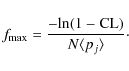
|
(1) |
We consider the mass and period power law indexes from Cumming et al. (2008)
![\begin{figure}
\par\includegraphics[width=8.5cm,clip]{11716fg13.ps}
\end{figure}](/articles/aa/full_html/2010/01/aa11716-09/img200.png)
|
Figure 11:
Top: survey mean detection probability derived as a
function of semi-major axis assuming parametric mass and period
distributions derived by Cumming et al. (2008), i.e. with
|
| Open with DEXTER | |
6.4 Limitations
Determination of detection thresholds (detailed previously), determination of the ages of young nearby stars, and the use of uncalibrated evolutionary models currently limit the relevancy of all statistical analyses of deep imaging surveys aimed at constraining the population of giant planets.
6.4.1 Age determination
Ages of young stars near the Sun are deduced based on photometric, spectroscopic and kinematic studies; various diagnostics are commonly used, depending on the spectral type and age of a given star. Details may be found in ZS04 and T08. In general, the most reliable ages are obtained for stars that can be placed reliably into a moving group or association.
Our sample is composed of 88 stars, including 51 members of known
young, nearby associations (TWA, ![]() Pic, Tuc-Hor and AB
Dor). Ages for the TWA and
Pic, Tuc-Hor and AB
Dor). Ages for the TWA and ![]() Pic associations have been
reasonably well constrained by various and independent studies (stellar
properties and dynamical trace-back):
8
-3+4 Myr (TWA; de la Reza et al. 2006; Barrado y Navasués
2006; Scholz et al. 2007) and 12
-4+8 Myr (
Pic associations have been
reasonably well constrained by various and independent studies (stellar
properties and dynamical trace-back):
8
-3+4 Myr (TWA; de la Reza et al. 2006; Barrado y Navasués
2006; Scholz et al. 2007) and 12
-4+8 Myr (![]() Pic,
Zuckerman et al. 2001b, Ortega et al. 2004) respectively. Isochrones,
lithium depletion and X-ray luminosoties indicate an age for Tuc-Hor
of 30 Myr (Zuckerman et al. 2001a). The age of the AB Dor association
is in some dispute (see Zuckerman et al. 2004; Luhman et al. 2005;
Luhman & Potter 2006; Lopez-Santiago et al. 2006; Janson et al. 2007; Ortega et al. 2007; Close et al. 2007; Boccaletti et al. 2008; Torres et al. 2008). In our simulations, we have assumed an age of 70 Myr for AB Dor stars.
Pic,
Zuckerman et al. 2001b, Ortega et al. 2004) respectively. Isochrones,
lithium depletion and X-ray luminosoties indicate an age for Tuc-Hor
of 30 Myr (Zuckerman et al. 2001a). The age of the AB Dor association
is in some dispute (see Zuckerman et al. 2004; Luhman et al. 2005;
Luhman & Potter 2006; Lopez-Santiago et al. 2006; Janson et al. 2007; Ortega et al. 2007; Close et al. 2007; Boccaletti et al. 2008; Torres et al. 2008). In our simulations, we have assumed an age of 70 Myr for AB Dor stars.
In our statistical analysis of 65 stars observed in coronagraphic imaging mode, 45 are confirmed members of known associations while 17 are young candidates, currently not identified as members of any kinematic group which makes an age estimate particularly difficult. An excellent example of a young star not known to be a member of the above listed moving groups is HR 8799, identified by Marois et al. (2008b) as orbited by 3 giant planets but with an age uncertainly between 30 and 160 Myr. In our analysis, age is directly used to convert the detection limits to mass using evolutionary models. Therefore, age determination remains a main limitation in this work and others to constrain reliably the properties of a putative population of giant planets around young, nearby stars.
6.4.2 Evolutionary models
Evolutionary model predictions are commonly used to infer substellar
masses from observed luminosities, as we did to convert our survey
detection sensitivity into planetary mass limits. For stars and brown
dwarfs formed by gravitational collapse and fragmentation, models
consider the idealized description of non-accreting systems
contracting at large initial radii. Remaining circumstellar material,
accretion and uncertainties related to choice of initial conditions
imply that comparison between observations and models are quite
uncertain at young ![]() 100 Myr ages (Baraffe et al. 2002). Such a
comparison might be rendered
even worse should young giant planets form by core-accretion (Marley
et al. 2007). Then massive giant planets might be significantly
fainter than equal-mass objects formed in isolation via gravitational
collapse. However, a critical issue is treatment of the accretion
shock through which most of the giant planet mass is processed and
which remains highly uncertain. In previous analyses of survey
detection sensitivities, only predictions from the Chabrier et al. (2000)
and Baraffe et al. (2003) models were used. Adoption of Burrows et al. (2003), assuming the same initial conditions, does not change
significantly the results (Nielsen et al. 2008).
100 Myr ages (Baraffe et al. 2002). Such a
comparison might be rendered
even worse should young giant planets form by core-accretion (Marley
et al. 2007). Then massive giant planets might be significantly
fainter than equal-mass objects formed in isolation via gravitational
collapse. However, a critical issue is treatment of the accretion
shock through which most of the giant planet mass is processed and
which remains highly uncertain. In previous analyses of survey
detection sensitivities, only predictions from the Chabrier et al. (2000)
and Baraffe et al. (2003) models were used. Adoption of Burrows et al. (2003), assuming the same initial conditions, does not change
significantly the results (Nielsen et al. 2008).
7 Conclusions
With NACO at the VLT we have conducted a deep adaptive optics imaging survey
of 88 nearby stars of the southern hemisphere. Our selection
criteria favored youth (![]() 100 Myr) and proximity to Earth (
100 Myr) and proximity to Earth (![]() 100 pc) to
optimize the detection of planetary mass companions. Known
visual binaries were excluded to avoid degrading the NACO AO and/or
coronagraphic detection performances. Among our sample, 51 stars are
members of young, nearby comoving groups. 32 are young, nearby stars
currently not identified as members of any currently known association
and 5 have been reclassified as older (
100 pc) to
optimize the detection of planetary mass companions. Known
visual binaries were excluded to avoid degrading the NACO AO and/or
coronagraphic detection performances. Among our sample, 51 stars are
members of young, nearby comoving groups. 32 are young, nearby stars
currently not identified as members of any currently known association
and 5 have been reclassified as older (![]() 100 Myr) systems. The
spectral types cover the sequence from B to M with
100 Myr) systems. The
spectral types cover the sequence from B to M with
![]() BAF stars,
BAF stars, ![]() GK stars and
GK stars and ![]() M dwarfs. The separations
investigated typically range between 0.1'' and 10'',
i.e. between 10 and 500 AU. A sample of 65 stars was
observed in deep coronagraphic imaging that enabled sensitivity to
star-planet luminosity contrasts
as large as 106 and, thus, to planetary mass
companions down to 1
M dwarfs. The separations
investigated typically range between 0.1'' and 10'',
i.e. between 10 and 500 AU. A sample of 65 stars was
observed in deep coronagraphic imaging that enabled sensitivity to
star-planet luminosity contrasts
as large as 106 and, thus, to planetary mass
companions down to 1
![]() (at 24% of our sample) and 3
(at 24% of our sample) and 3
![]() (at
67%). We used a standard observing sequence to measure precisely the
position and the flux of all detected infrared sources relative to their
youthful primary stars. Observations at several epochs enabled us to
discriminate comoving companions from background objects. The main
results are:
(at
67%). We used a standard observing sequence to measure precisely the
position and the flux of all detected infrared sources relative to their
youthful primary stars. Observations at several epochs enabled us to
discriminate comoving companions from background objects. The main
results are:
- -
- Discovery of 17 new close (0.1-5.0'') multiple
systems. HIP 108195 AB and C (F1III-M6), HIP 84642 AB
(
 AU, K0-M5) and TWA22 AB (
 AU; M6-M6) are
confirmed as comoving systems. TWA22 AB, with 80% of its orbit
already resolved, is likely to be a rare astrometric calibrator for
testing evolutionary model predictions.
AU; M6-M6) are
confirmed as comoving systems. TWA22 AB, with 80% of its orbit
already resolved, is likely to be a rare astrometric calibrator for
testing evolutionary model predictions.
- -
- About 236 faint candidate companions were detected around 36 stars observed in coronagraphic mode. Follow-up observations with VLT or HST for 30 stars enabled us to identify the status of these candidates. 1% are confirmed as comoving companions, 43% are identified as probable background contaminants and about 56% require further follow-up observations (these come mostly from crowded fields near six stars observed at one epoch).
- -
- Confirmation of previously discovered substellar companions around GSC 08047-00232, AB Pic and 2M1207.
- -
- A statistical analysis of the complete set of detection limits
enables us to constrain at semi-major axes from 20 to a few 100 AU,
various mass, period and eccentricity distributions of giant planets
extrapolated and normalized from RV surveys. Limits are derived on
the occurence of giant planets for a given set of physical and orbital
distributions; the survey begins to constrain significantly the
population of giant planets with masses
 3
3
 and with semimajor axes 40 AU.
We thank the ESO Paranal staff for performing the service mode observations. We also acknowledge partial financial support from the PNPS and Agence National de la Recherche, in France, from INAF through PRIN 2006 ``From disk to planetray systems: understanding the origin and demographics of solar and extrasolar planetary systems'' and from NASA in the USA. We also would like to thanks France Allard and Isabelle Baraffe for their inputs on evolutionary models and synthetic spectral libraries. Finally, our anonymous referee for her/his detailed and very constructive report.
References
- Baraffe, I., Chabrier, G., Allard, F., & Hauschildt, P. H. 2002, A&A 382, 563 [Google Scholar]
- Baraffe, I., Chabrier, G., Barman, T. S., Allard, F., & Hauschildt, P. H. 2003, A&A, 402, 701 [Google Scholar]
- Barrado, Y., & Navascués, D. 2006, A&A, 459, 511 [Google Scholar]
- Biller, B. A., Close, L. M., Masciadri, E., et al. 2007, ApJS, 173, 143 [NASA ADS] [CrossRef] [Google Scholar]
- Boccaletti, A., Chauvin, G., Baudoz, P., & Beuzit, J.-L. 2008, A&A, 482, 939 [Google Scholar]
- Boley, A. C. 2009, ApJ, 695, L53 [NASA ADS] [CrossRef] [Google Scholar]
- Bonnell, I. A., Larson, R. B., & Zinnecker, H. 2007, Protostars and Planets V, 951, 149 [NASA ADS] [Google Scholar]
- Burgasser, A. J., Kirkpatrick, J. D., Brown, M. E., et al. 1999, ApJ, 522, 65 [Google Scholar]
- Burgasser, A. J., Reid, I. N., Siegler, N., et al. 2007, Protostars and Planets V, 951, 427 [NASA ADS] [Google Scholar]
- Burrows, A., Sudarsky, D., & Lunine, J. I. 2003, ApJ, 596, 587 [NASA ADS] [CrossRef] [Google Scholar]
- Butler, R. P., Wright, J. T., Marcy, G. W., et al. 2006, ApJ, 646, 505 [NASA ADS] [CrossRef] [Google Scholar]
- Carson, J. C., Eikenberry, S. S., Brandl, B. R., Wilson,, J. C., & Hayward, T. L. 2005, AJ, 130, 1212 [NASA ADS] [CrossRef] [Google Scholar]
- Carson, J. C., Eikenberry, S. S., Smith, J. J., & Cordes, J. M. 2006, AJ, 132, 1146 [NASA ADS] [CrossRef] [Google Scholar]
- Chabrier, G., Baraffe, I., Allard, F., & Hauschildt, P. H. 2000, ApJ, 542, 464 [NASA ADS] [CrossRef] [Google Scholar]
- Chauvin, G., Thomson, M., Dumas, C., et al. 2003, A&A, 404, 157 [Google Scholar]
- Chauvin, G., Lagrange, A.-M., Dumas, C., et al. 2004, A&A, 425, L25 [Google Scholar]
- Chauvin, G., Lagrange, A.-M., Lacombe, F., et al. 2005a, A&A, 430, 1027 [Google Scholar]
- Chauvin, G., Lagrange, A.-M., Dumas, C., et al,, 2005b, A&A, 438, L25 [Google Scholar]
- Chauvin, G., Lagrange, A.-M., Zuckerman, B., et al. 2005c, A&A, 438, L29 [Google Scholar]
- Chauvin, G., Lagrange, A.-M., Udry, S., et al. 2006, A&A, 456, 1165 [Google Scholar]
- Close, Laird, M., Thatte, N., Nielsen, E. L., et al. 2007, ApJ, 665, 736 [NASA ADS] [CrossRef] [Google Scholar]
- Couteau, P. 1960, J. Obs., 43, 13 [NASA ADS] [Google Scholar]
- Cumming, A., Butler, R. P., Marcy, G. W., et al. 2008, PASP, 120, 531 [NASA ADS] [CrossRef] [Google Scholar]
- de la Reza, R., Jilinski, E., & Ortega, V. G. 2006, AJ, 131, 2609 [NASA ADS] [CrossRef] [Google Scholar]
- Delfosse, X., Tinney, C. G., Forveille, T., et al. 1997, A&A, 327, 25 [Google Scholar]
- Devillar, N. 1997, The messenger, 87 [Google Scholar]
- Dohlen, K., Beuzit, J.-L., Feldt, M., et al. 2006, SPIE, 6269, 24 [NASA ADS] [Google Scholar]
- Dommanget, J., & Nys, O. 2000, A&A, 363, 991 [Google Scholar]
- Ducourant, C., Teixeira, R., Chauvin, G., et al. 2008, A&A, 477, L1 [Google Scholar]
- Eggenberger, A., Udry, S., Chauvin, G., et al. 2007, A&A, 474, 273 [Google Scholar]
- Endl, M., Cochran, W. D., Krster, M., et al. 2006, ApJ, 649, 436 [NASA ADS] [CrossRef] [Google Scholar]
- Epchtein, N., de Batz, B., Capoani, L., et al. 1997, Msngr, 87, 27 [Google Scholar]
- Fuhrmeister, B., & Schmitt, J. H. M. M. 2003, A&A, 403, 247 [Google Scholar]
- Gizis, J., Jao, W., Subsavage, J. P., & Henry, T. J., 2007, ApJ, 669, L45 [NASA ADS] [CrossRef] [Google Scholar]
- Goldman, B., Delfosse, X., Forveille, T., et al. 1999, A&A, 351, L5 [Google Scholar]
- Grether, D., & Lineweaver, C. H., 2006, ApJ, 640, 1051 [NASA ADS] [CrossRef] [Google Scholar]
- Grillmair, C. J., Burrows, A., Charbonneau, D., et al. 2008, Nature, 456, 767 [NASA ADS] [CrossRef] [PubMed] [Google Scholar]
- Itoh, Y., Hayashi, M., Tamura, M., et al. 2005, ApJ, 620, 984 [NASA ADS] [CrossRef] [Google Scholar]
- Janson, M., Brandner, W., Lenzen, R., et al. 2007, A&A, 462, 615 [Google Scholar]
- Joergens, V. 2006, A&A, 446, 1165 [Google Scholar]
- Johnson, J. A., Fischer, D. A., Marcy, G. W., et al. 2007, ApJ, 665, 785 [NASA ADS] [CrossRef] [Google Scholar]
- Kalas, P., Graham, J. R., Chiang, E., et al. 2008, Science, 322, 1345 [NASA ADS] [CrossRef] [PubMed] [Google Scholar]
- Kastner, J. H., Zuckerman, B., Weintraub, D. A., & Forveille, T. 1997, Science, 277, 67 [NASA ADS] [CrossRef] [PubMed] [Google Scholar]
- Kasper, M., Apai, D., Janson, M., & Brandner, W. 2007, A&A, 472, 321 [Google Scholar]
- Kirkpatrick, J. D., Reid, I. N., Liebert, J., et al. 1999, ApJ, 519, 802 [NASA ADS] [CrossRef] [Google Scholar]
- Kirkpatrick, J. D., Reid, I. N., Liebert, J., et al. 2000, ApJ, 120, 447 [Google Scholar]
- Lafrenière, D., Doyon, R., Marois, C., et al. 2007, ApJ, 670, 1367 [NASA ADS] [CrossRef] [Google Scholar]
- Lafrenière, D., Jayawardhana, R., van Kerkwijk, M. H., et al. 2008, ApJ, 689, 153 [Google Scholar]
- Lagrange, A.-M., Desort, M., Galland, F., Udry, S., & Mayor, M. 2009a, A&A, 495, 335 [Google Scholar]
- Lagrange, A.-M., Gratadour, D., Chauvin, G., et al. 2009b, A&A, 493, L21 [Google Scholar]
- Lenzen, R., Hofmann, R., Bizenberger, P., & Tusche, A. 1998, SPIE, 3354, 606 [Google Scholar]
- López-Santiago, J., Montes, D., Crespo-Chacón, I., & Fernández-Figueroa, M. J. 2006, ApJ, 643, 1160 [NASA ADS] [CrossRef] [Google Scholar]
- Lowrance, P. J., McCarthy, C., Becklin, E. E., et al. 1999, ApJ, 512, L69 [NASA ADS] [CrossRef] [Google Scholar]
- Lowrance, P. J., Schneider, G., Kirkpatrick, J., et al. 2000, ApJ, 541, L390 [NASA ADS] [CrossRef] [Google Scholar]
- Lowrance, P. J., Becklin, E. E., Schneider, G., et al. 2005, AJ, 130, 1845 [NASA ADS] [CrossRef] [Google Scholar]
- Luhman, K., & Jayawardhana, R., 2002, ApJ, 566, 1132 [NASA ADS] [CrossRef] [Google Scholar]
- Luhman, K. L., & Potter, D. 2006, ApJ, 638, 887 [NASA ADS] [CrossRef] [Google Scholar]
- Luhman, K. L., Stauffer, J. R., & Mamajek, E. E. 2005, 628, L69 [Google Scholar]
- Luhman, K. L., Wilson, J. C., Brandner, W., et al. 2006, ApJ, 649, 894 [NASA ADS] [CrossRef] [Google Scholar]
- Marcy, G., Butler, R. P., Fischer, D., et al. 2005, PThPS, 158, 24 [Google Scholar]
- Marley, M. S., Fortney, J. J., Hubickyj, O., Bodenheimer, P., & Lissauer, J. J. 2007, ApJ, 655, 541 [NASA ADS] [CrossRef] [Google Scholar]
- Marois, C., Lafrenière, D., Macintosh, B., & Doyon, R., 2008a, ApJ, 673, 647 [NASA ADS] [CrossRef] [Google Scholar]
- Marois, C., Macintosh, B., Barman, T., et al. 2008b, Science, 322, 1348 [NASA ADS] [CrossRef] [PubMed] [Google Scholar]
- Masciadri, E., Mundt, R., Henning, Th., & Alvarez, C. 2005, ApJ, 625, 1004 [NASA ADS] [CrossRef] [Google Scholar]
- Mayor, M., & Queloz, D. 1995, Nature, 378, 355 [NASA ADS] [CrossRef] [Google Scholar]
- McCarthy, C., & Zuckerman, B. 2004, AJ, 127, 2871 [NASA ADS] [CrossRef] [Google Scholar]
- McCaughrean, M. J., & Stauffer, J. R. 1994, AJ, 108, 1382 [NASA ADS] [CrossRef] [Google Scholar]
- Macintosh, B., Troy, M., Doyon, R., et al. 2006, SPIE, 6272, 20 [NASA ADS] [Google Scholar]
- Metchev, S., & Hillenbrand, L. 2006, ApJ, 651, 1166 [NASA ADS] [CrossRef] [Google Scholar]
- Metchev, S., & Hillenbrand, L. 2008, ApJ, 676, 1281 [NASA ADS] [CrossRef] [Google Scholar]
- Mohanty, S., Jayawardhana, R., Huélamo, N., & Mamajek, E. 2007, ApJ, 657, 1064 [NASA ADS] [CrossRef] [Google Scholar]
- Mugrauer, M., Seifahrt, A., & Neuhäuser, R. 2007, MNRAS, 378, 1328 [NASA ADS] [CrossRef] [Google Scholar]
- Nakajima, T., Oppenheimer, B. R., Kulkarni, S. R., et al. 1995, Nature, 378, 463 [NASA ADS] [CrossRef] [Google Scholar]
- Neuhäuser, R., & Guenther, E. W. 2004, A&A, 420, 647 [Google Scholar]
- Neuhäuser, R., Guenther, E. W., Alves, J., et al. 2003, AN, 324, 535 [Google Scholar]
- Neuhäuser, R., Guenther, E. W., Wuchterl, G., et al. 2005, A&A, 435, 13 [Google Scholar]
- Nielsen, E. L., Close, L. M., Biller, B. A., Masciadri, E., & Lenzen, R., 2008, ApJ, 674, 466 [Google Scholar]
- Ortega, V. G., de la Reza, R., Jilinski, E., & Bazzanella, B. 2004, ApJ, 609, 243 [NASA ADS] [CrossRef] [Google Scholar]
- Ortega, V. G., Jilinski, E., de La Reza, R., & Bazzanella, B. 2007, MNRAS, 377, 441 [NASA ADS] [CrossRef] [Google Scholar]
- Papaloizou, J. C. B., & Terquem, C. 2001, MNRAS, 325, 221 [NASA ADS] [CrossRef] [Google Scholar]
- Patience, J., White, R. J., Ghez, A. M., et al. 2002, ApJ, 581, 654 [NASA ADS] [CrossRef] [Google Scholar]
- Rafikov, R. R. 2005, ApJ, 621, L69 [NASA ADS] [CrossRef] [Google Scholar]
- Rousset, G., Lacombe, F., Puget, P., et al., 2002, SPIE, 4007 [Google Scholar]
- Schmidt, T. O. B., Neuhäuser, R., Seifahrt, A., et al. 2008, A&A, 491, 311 [Google Scholar]
- Scholz, A., Coffey, J., Brandeker, A., & Jayawardhana, R. 2007, ApJ, 662, 1254 [NASA ADS] [CrossRef] [Google Scholar]
- Siess, L., Dufour, E., & Forestini, M. 2000, A&A, 358, 593 [Google Scholar]
- Skrutskie, M. F., Schneider, S. E., Stiening, R., et al. 1997, ASSL, 210, 25 [NASA ADS] [Google Scholar]
- Song, I., Zuckerman, B., & Bessel, M. S. 2003, ApJ, 599, 342 [Google Scholar]
- Song, I., Schneider, G., Zuckerman, B., et al. 2006, ApJ, 26, 282 [Google Scholar]
- Swain, M. R., Vasisht, G., & Tinetti, G. 2008, Nature, 452, 329 [NASA ADS] [CrossRef] [PubMed] [Google Scholar]
- Torres, C. A. O., Quast, G. R., Melo, C. H. F., & Sterzik, M. F. 2008, Handbook of Star Forming Regions, Volume II: The Southern Sky, ASP Monograph Publications, 5, 757 (T08) [Google Scholar]
- Udry, S., & Santos, N. C. 2007, ARA&A, 45, 397 [Google Scholar]
- van Dessel, E., & Sinachopoulos, D. 1993, A&AS, 100, 517 [Google Scholar]
- Véran, J. P., & Rigaut, F. 1998, SPIE, 3353, 426 [Google Scholar]
- Webb, R. A., Zuckerman, B., Platais, I., et al. 1999, ApJ, 512, L63 [NASA ADS] [CrossRef] [Google Scholar]
- Wilson, J. C., Kirkpatrick, J. D., Gizis, J. E., et al. 2001, AJ, 122, 1989 [NASA ADS] [CrossRef] [Google Scholar]
- York, D. G., Adelman, J., Anderson, J. E. Jr, et al. 2000, AJ, 120, 1579 [Google Scholar]
- Zuckerman, B., & Song, I. 2004, ARA&A, 42, 685 (ZS04) [Google Scholar]
- Zuckerman, B., & Song, I. 2009, A&A, 493, 1149 [Google Scholar]
- Zuckerman, B., Song, I., & Webb, R. A. 2001a, ApJ, 559, 388 [NASA ADS] [CrossRef] [Google Scholar]
- Zuckerman, B., Song, I., Bessell, M. S., & Webb, R. A. 2001b, ApJ, 562, 87 [Google Scholar]
- Zuckerman, B., Song, I., & Bessell, M. S., 2004, ApJ, 613, L65 [NASA ADS] [CrossRef] [Google Scholar]
Footnotes
- ... stars
- Table 8 is only available in electronic form at the CDS via anonymous ftp to cdsarc.u-strasbg.fr (130.79.128.5) or via http://cdsweb.u-strasbg.fr/cgi-bin/qcat?J/A+A/509/A52
- ...
NACO
- http://www.eso.org/instruments/naos/
- ...

- See filters description: http://www.eso.org/instruments/naco/inst/filters.html
- ...
decade
- http://www.eso.org/gen-fac/pubs/astclim/paranal/seeing/adaptive-optics/statfwhm.html
- ...Eclipse
- http://www.eso.org/projects/aot/eclipse/
All Tables
Table 1: Deep imaging surveys of young (<100 Myr), nearby (<100 pc) stars dedicated to the search for planetary mass companions and published in the literature.
Table 2: Sample of southern young, nearby stars observed during our VLT/NACO deep imaging survey.
Table 3: Sample of southern young, nearby stars observed.
Table 4: Summary of the different observing campaigns of our survey.
Table 5: Mean plate scale and true north orientation for each observing run.
Table 6:
Relative positions and ![]() and H-band contrast of the new
binaries resolved by NACO at VLT.
and H-band contrast of the new
binaries resolved by NACO at VLT.
Table 7:
Properties of the confirmed comoving substellar companions discovered
in the young, nearby associations: TW Hydrae (TWA), ![]() Pictoris
(
Pictoris
(![]() Pic), Columba (Col) and Carina (Car).
Pic), Columba (Col) and Carina (Car).
All Figures
|
|
Figure 1:
Histrograms summarizing the main properties of the sample of
young, nearby stars observed with NACO at VLT. Top-left:
histogram of spectral types for the stars observed in coronagraphic
imaging (crossed lines) and in direct imaging (simple
lines). Top-middle: histogram of ages for members of known
young, nearby associtations (TWA, |
| Open with DEXTER | |
| In the text | |
|
|
Figure 2:
VLT/NACO adaptive optics system performances. Strehl ratio at
2.20 |
| Open with DEXTER | |
| In the text | |
|
|
Figure 3:
Left: VLT/NACO corongraphic image of HIP 95270
obtained in H-band with the S13 camera. The small (
|
| Open with DEXTER | |
| In the text | |
|
|
Figure 4:
Left: VLT/NACO coronagraphic detection limits in
H-band (combined with the S13 camera). The median detection limits are
given for different target spectral types (BAF, GK and M stars) and for
the 0.7'' (solid line) and 1.4'' (dash dotted
line) coronagraphic masks. Right: VLT/NACO coronagraphic
detection limits in |
| Open with DEXTER | |
| In the text | |
|
|
Figure 5:
VLT/NACO coronagraphic detection limits in |
| Open with DEXTER | |
| In the text | |
|
|
Figure 6: VLT/NACO Measurements (filled circles with uncertainties) of the offset positions of a comoving companion AB Pic b to the primary star ``A'' (left) and of a CC relative to 0ES1847 (right). For each diagram, the expected variation of offset positions, if the candidate is a background object, is shown (curved line). The variration is estimated based on the parallactic and proper motions of the primary star, as well as the initial offset position of the CC from A. The empty squares give the corresponding expected offset positions of a background object for various epochs of observations (with uncertainties). In the case of AB Pic b, the relative positions do not change with time confirming that AB Pic b is comoving. On the contrary, the relative position of the CC to 0ES1847 varies in time as predicted for a stationary background object. For our sample, astrometric follow-up over 1-2 years enabled a rapid identification of true companions. |
| Open with DEXTER | |
| In the text | |
|
|
Figure 7: New visual binaries resolved with NACO at VLT. HIP 108195 AB, HIP 84642 AB and TWA22 AB were in addition confirmed as comoving multiple systems. TWA22 AB was monitored for 4 years to constrain the binary orbit and determine its total dynamical mass (see Bonnefoy et al. 2009, accepted). |
| Open with DEXTER | |
| In the text | |
|
|
Figure 8:
Composite VLT/NACO |
| Open with DEXTER | |
| In the text | |
|
|
Figure 9:
Histogram of projected physical separations explored, for
various planetary masses (1, 3, 5, 7, 10 and 13)
|
| Open with DEXTER | |
| In the text | |
|
|
Figure 10:
Non-detection probability for our survey, based on various
sets of period and mass distributions as a function of the semi-major
axis cut-off of the period distribution. Mass and period distributions
are extrapolated and normalized from RV studies. Top:
variation of the non-detection probability with |
| Open with DEXTER | |
| In the text | |
|
|
Figure 11:
Top: survey mean detection probability derived as a
function of semi-major axis assuming parametric mass and period
distributions derived by Cumming et al. (2008), i.e. with
|
| Open with DEXTER | |
| In the text | |
Copyright ESO 2010
Current usage metrics show cumulative count of Article Views (full-text article views including HTML views, PDF and ePub downloads, according to the available data) and Abstracts Views on Vision4Press platform.
Data correspond to usage on the plateform after 2015. The current usage metrics is available 48-96 hours after online publication and is updated daily on week days.
Initial download of the metrics may take a while.