| Issue |
A&A
Volume 508, Number 3, December IV 2009
|
|
|---|---|---|
| Page(s) | 1193 - 1204 | |
| Section | Cosmology (including clusters of galaxies) | |
| DOI | https://doi.org/10.1051/0004-6361/200912906 | |
| Published online | 04 November 2009 | |
A&A 508, 1193-1204 (2009)
Bispectrum covariance in the flat-sky limit
B. Joachimi1,2 - X. Shi1 - P. Schneider1
1 - Argelander-Institut für Astronomie (AIfA), Universität Bonn, Auf dem Hügel 71, 53121 Bonn, Germany
2 - Department of Physics and Astronomy, University College London, London WC1E 6BT, UK
Received 16 July 2009 / Accepted 20 October 2009
Abstract
Aims. To probe cosmological fields beyond the Gaussian
level, three-point statistics can be used, all of which are related to
the bispectrum. Hence, measurements of CMB anisotropies, galaxy
clustering, and weak gravitational lensing alike have to rely upon an
accurate theoretical background concerning the bispectrum and its noise
properties. If only small portions of the sky are considered, it is
often desirable to perform the analysis in the flat-sky limit. We aim
at a formal, detailed derivation of the bispectrum covariance in the
flat-sky approximation, focusing on a pure two-dimensional
Fourier-plane approach.
Methods. We define an unbiased estimator of the bispectrum,
which takes the average over the overlap of annuli in Fourier space,
and compute its full covariance. The outcome of our formalism is
compared to the flat-sky spherical harmonic approximation in terms of
the covariance, the behavior under parity transformations, and the
information content. We introduce a geometrical interpretation of the
averaging process in the estimator, thus providing an intuitive
understanding.
Results. Contrary to foregoing work, we find a difference by a
factor of two between the covariances of the Fourier-plane and the
spherical harmonic approach. We argue that this discrepancy can be
explained by the differing behavior with respect to parity. However, in
an exemplary analysis it is demonstrated that the Fisher information of
both formalisms agrees to high accuracy. Via the geometrical
interpretation we are able to link the normalization in the bispectrum
estimator to the area enclosed by the triangle configuration at
consideration as well as to the Wigner symbol, which leads to
convenient approximation formulae for the covariances of both
approaches.
Key words: methods: statistical - cosmology: theory - cosmological parameters
1 Introduction
As the concordance model of cosmology becomes more and more consolidated, the focus increasingly turns towards probing effects beyond the standard paradigm, such as non-Gaussian initial conditions or the evolution of the large-scale structure in the highly non-linear regime. To lowest order, these effects can be measured by three-point statistics of the underlying fields, all of which are related to the bispectrum. Hence, work in both theory and observations concerning the bispectrum and its noise properties has been undertaken for CMB measurements (e.g. Cooray et al. 2008; Hu 2000), galaxy clustering surveys (e.g. Scoccimarro 2000; Scoccimarro et al. 2001; Sefusatti et al. 2006), or, more recently, weak gravitational lensing on cosmological scales (e.g. Takada & Jain 2004; Bernardeau et al. 2002b; Jarvis et al. 2004).
While theoretical computations at the bispectrum level are already considerably more demanding than for second-order statistics, this does apply even more so to the bispectrum covariance, which is a six-point statistic. On the full sky calculations are done by expanding the signal into spherical harmonics. If only small angular scales are considered, it is often more convenient to use a flat-sky approximation and work in terms of Fourier amplitudes. In the case of weak lensing the flat-sky limit is appropriate for practically all applications because signal correlations can only be measured up to separations of a few degrees.
Although other approaches exist in the literature (e.g. Sefusatti et al. 2006; Matarrese et al. 1997), a lot of work is done within a flat-sky spherical harmonic formalism (Hu 2000), which suffers - at least formally - from drawbacks. For instance, the resulting flat-sky expressions are valid only for integer arguments and thus for a bin width of unity, whereas it is desirable to evaluate the bispectrum and its covariance at real-valued angular frequencies and e.g. a logarithmic binning. The formulae still contain Wigner symbols whose physical meaning within a flat-sky consideration remain obscure. As the spherical harmonic expansion can only be done on the full unit sphere, the finite size of the survey at consideration is usually accounted for by multiplying a factor, containing the sky coverage, by hand. Moreover, the accuracy of some of the approximations in the transition between full sky and two-dimensional plane (see Hu 2000) is uncertain.
This work aims at clarifying the derivation of bispectrum covariances in the flat-sky limit. We attempt to do so by presenting a detailed calculation which is purely based on the two-dimensional Fourier formalism, followed by a comparison of this approach with the flat-sky spherical harmonic results in terms of their covariance, the behavior under parity transformations, and the information content. Moreover, we provide further insight and illustration by establishing relations between Wigner symbols, the averaging process in the bispectrum estimator, and a geometrical view.
The outline of this note is as follows: in Sect. 2 a bispectrum estimator is defined and shown to be unbiased. Section 3 introduces a geometrical interpretation, which is then applied to deal with the issue of degenerate triangle configurations. In Sect. 4 the covariance of the estimator defined beforehand is computed. The result is compared with the spherical harmonics approach and demonstrated to be equivalent in terms of information content in Sect. 5. To explain the differences between the covariances, we also discuss the treatment of parity in both formalisms. We summarize our findings and conclude in Sect. 6. To avoid confusion, we refrain from using the term ``flat sky'' in the following, but refer to our formalism as ``Fourier-plane'' and to the approach as e.g. given in Hu (2000) as ``spherical harmonic'' (both are flat-sky approximations).
2 Bispectrum estimator
We consider a continuous, two-dimensional random field g with mean zero, which is characterized by its complex Fourier amplitudes
![]() ,
where
,
where
![]() denotes the angular frequency vector. Throughout, it will be assumed
that this field is statistically homogeneous, i.e. invariant under
translations, and statistically isotropic, i.e. invariant under
rotations. In a cosmological context g
could for instance represent the temperature fluctuations of the CMB,
the number density contrast of galaxy surveys, or the weak lensing
convergence.
denotes the angular frequency vector. Throughout, it will be assumed
that this field is statistically homogeneous, i.e. invariant under
translations, and statistically isotropic, i.e. invariant under
rotations. In a cosmological context g
could for instance represent the temperature fluctuations of the CMB,
the number density contrast of galaxy surveys, or the weak lensing
convergence.
In what follows we will largely follow the approach of Joachimi et al. (2008), assuming likewise measurements in a compact, contiguous survey of size A. We will restrict our considerations to an angular extent much smaller than the size of the survey, i.e. to
![]() ,
where
,
where
![]() is the maximum separation allowed by the survey geometry. Boundary effects due to the finite field size, as e.g. discussed in Joachimi et al. (2008) for the second-order level, can then be safely neglected.
is the maximum separation allowed by the survey geometry. Boundary effects due to the finite field size, as e.g. discussed in Joachimi et al. (2008) for the second-order level, can then be safely neglected.
Furthermore, we will not explicitly consider additional noise terms due to the discrete sampling of the continuous field g,
for ease of notation. To account for these shot noise or, in the case
of weak lensing, shape noise terms in the covariance, they can simply
be added to the second-order measures, so in this Fourier space
approach, to the power spectra (e.g. Hu 1999; Kaiser 1998).
Note that the galaxy ellipticity, and not the convergence ![]() ,
is the direct observable in weak lensing. However, in absence of shape noise and for
,
is the direct observable in weak lensing. However, in absence of shape noise and for
![]() ,
the estimators in terms of the galaxy ellipticity, as given in Joachimi et al. (2008), can be re-written directly in terms of
,
the estimators in terms of the galaxy ellipticity, as given in Joachimi et al. (2008), can be re-written directly in terms of ![]() .
Thus, without loss of generality, one can consider the convergence as the observable that the estimator is based on.
.
Thus, without loss of generality, one can consider the convergence as the observable that the estimator is based on.
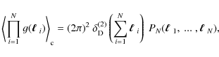
For a statistically homogeneous and isotropic random field one defines the bispectrum as
where
Similarly to Joachimi et al. (2008),
we construct an estimator of the bispectrum by averaging configurations
over annuli, where here one has the complication of allowing only those
combinations of angular frequency vectors that form a triangle. The
area of an annulus with mean radius
![]() is given by
is given by
with the bin size
where
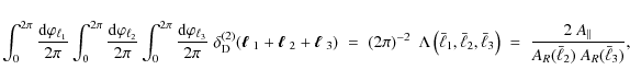
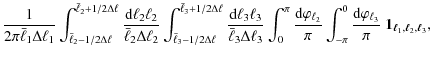
In the following, we demonstrate that (3) is unbiased by computing the ensemble average,


In the first step the definition of the bispectrum (3) was inserted. The appearance of a squared delta-distribution requires taking into account the finite survey size. As shown in Joachimi et al. (2008), one can identify
which results in the second equality of (4).
Since the bispectrum only depends on the magnitudes of the angular
frequency vectors we can perform the integrations over the polar angles
of the
![]() -integrals. If
-integrals. If
![]() denotes the polar angle of
denotes the polar angle of
![]() ,
one gets
,
one gets


After inserting one possible representation of the delta-distribution in the first equality, we have made use of the definition of the Bessel function of the first kind of order 0,
The result of the integral over three Bessel functions is taken from Gradshteyn et al. (2000), formula No. 6.578.9, where we have defined
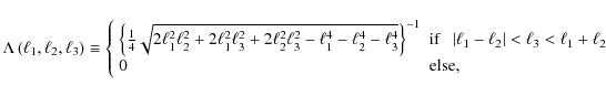
i.e. if
Inserting (6) into (4), one obtains
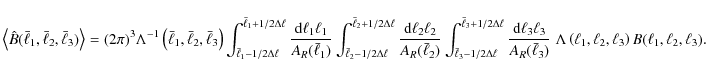
Analogous to the derivation at the level of second-order statistics (Joachimi et al. 2008) we assume now that the annuli are thin enough such that
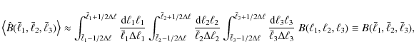
where in the last step the bin-averaged bispectrum was defined. Hence, (3) defines an unbiased estimator of the bispectrum. Following the restrictions on (6), this estimator is non-zero if the condition
3 Averaging over triangles
A central step in the construction of the bispectrum estimator (3) is the correct treatment of the averaging over annuli, given the triangle condition. This section provides an illustrative, geometrical interpretation of the averaging process and applies this view to a practical treatment of degenerate triangle configurations.
3.1 Geometrical interpretation
![\begin{figure}
\par\includegraphics[scale=.21]{12906fg1.ps}
\end{figure}](/articles/aa/full_html/2009/48/aa12906-09/img59.png)
|
Figure 1:
Sketch of the annuli and their overlap for fixed
|
| Open with DEXTER | |
Without loss of generality consider
![]() to be fixed. Due to the assumed statistical isotropy of the underlying random field the angular integration over
to be fixed. Due to the assumed statistical isotropy of the underlying random field the angular integration over
![]() is expected to simply reduce to an average over all directions of
is expected to simply reduce to an average over all directions of
![]() .
Then the geometric situation in the Fourier plane can be seen as in Fig. 1. For a given triangle, composed of the mean vectors
.
Then the geometric situation in the Fourier plane can be seen as in Fig. 1. For a given triangle, composed of the mean vectors
![]() ,
,
![]() ,
,
![]() with lengths
with lengths
![]() for
for
![]() ,
the annuli for
,
the annuli for
![]() and
and
![]() are shown. Due to the triangle condition, the average is not taken over
the whole area of the annuli, but merely over the region that the
annuli have in common. This area of overlap is well approximated by a
parallelogram of size
are shown. Due to the triangle condition, the average is not taken over
the whole area of the annuli, but merely over the region that the
annuli have in common. This area of overlap is well approximated by a
parallelogram of size
![]() ,
where
,
where ![]() is the internal angle of the triangle opposite
is the internal angle of the triangle opposite
![]() .
This relation can readily be computed from the geometry of the sketch and by noting
.
This relation can readily be computed from the geometry of the sketch and by noting
![]() .
.
The configuration is mirror-symmetric with respect to an axis through
![]() .
Correspondingly, another area of overlap of the same size, which is connected to the triangle
.
Correspondingly, another area of overlap of the same size, which is connected to the triangle
![]() ,
,
![]() ,
,
![]() ,
contributes as well. Noting that axis reflection is in two dimensions
equivalent to the parity transformation, the averaging is performed
over triangles of both parities. A detailed discussion on this issue is
given in Sect. 5.2.
,
contributes as well. Noting that axis reflection is in two dimensions
equivalent to the parity transformation, the averaging is performed
over triangles of both parities. A detailed discussion on this issue is
given in Sect. 5.2.
As the angle ![]() can also be related to the size of the triangle at consideration,
can also be related to the size of the triangle at consideration,
![]() ,
one finds the following correspondence of expressions:
,
one finds the following correspondence of expressions:
where the first equality is an immediate consequence of (6). To arrive at the last expression, we used (2). Hence, the angular integration over the delta-distribution yields the ratio of the area of overlap
Two approximations are involved in this picture. First, the shaded regions in Fig. 1
are approximated as parallelograms, which is a good assumption if the
angle, at which the two annuli intersect, does not become too small.
Moreover, the narrower the annuli, the less discrepancy between the
area of the parallelogram and the actual overlap is expected. If the
triangle approaches the degenerate case, where
![]() and
and
![]() eventually come to lie on
eventually come to lie on
![]() ,
the area of overlap attains a more complex shape. In particular, the
correspondence to the area of the triangle, whose inverse is divergent,
does not hold anymore. Second, reconsidering (9), we have replaced the average of
,
the area of overlap attains a more complex shape. In particular, the
correspondence to the area of the triangle, whose inverse is divergent,
does not hold anymore. Second, reconsidering (9), we have replaced the average of ![]() over triangle side lengths by
over triangle side lengths by ![]() ,
evaluated at the average side lengths. This approximation similarly
breaks down for thick annuli and configurations in which a small change
in the length of an angular frequency vector causes a strong change in
the size of the overlap region, as is the case near degeneracy.
,
evaluated at the average side lengths. This approximation similarly
breaks down for thick annuli and configurations in which a small change
in the length of an angular frequency vector causes a strong change in
the size of the overlap region, as is the case near degeneracy.
![\begin{figure}
\par\includegraphics[scale=.61,angle=270]{12906fg2.ps}
\vspace*{-2mm}
\end{figure}](/articles/aa/full_html/2009/48/aa12906-09/img76.png)
|
Figure 2:
Comparison of expressions for the overlap area of annuli. Left panel: relative deviation of (12) from the overlap area of the annuli as a function of angular frequency. The bin width is kept constant at
|
| Open with DEXTER | |
In Fig. 2, we have plotted the relative deviation of
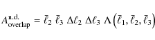
from the actual area of the overlap region, which we calculated numerically. For simplicity, we assume a constant bin width
3.2 Degenerate triangles
As discussed in the foregoing section, the approximations made in
the course of the construction of the bispectrum estimator break down
for degenerate triangle configurations. Equation (11) becomes invalid, the inverse area of the triangle ![]() diverging. Yet, to be of practical use, it is necessary to extend the validity of (3) to the case of degenerate triangles. We do so by making use of the geometrical interpretation of the averaging process.
diverging. Yet, to be of practical use, it is necessary to extend the validity of (3) to the case of degenerate triangles. We do so by making use of the geometrical interpretation of the averaging process.
![\begin{figure}
\par\includegraphics[scale=.22]{12906fg3.ps}
\end{figure}](/articles/aa/full_html/2009/48/aa12906-09/img81.png)
|
Figure 3:
Sketch of the region averaged over in case of a degenerate triangle, again for fixed
|
| Open with DEXTER | |
Still keeping
![]() fixed, consider the situation of a degenerate triangle as sketched in Fig. 3. Here,
fixed, consider the situation of a degenerate triangle as sketched in Fig. 3. Here,
![]() ,
while the depicted triangle has side lengths
,
while the depicted triangle has side lengths
![]() ,
,
![]() ,
and
,
and
![]() .
Again, we identify a parallelogram that serves as an approximation for
the overlap of the annuli, although, as the sketch suggests, with
considerably lower accuracy. The relation between the internal angle
.
Again, we identify a parallelogram that serves as an approximation for
the overlap of the annuli, although, as the sketch suggests, with
considerably lower accuracy. The relation between the internal angle ![]() of the triangle to the internal angle of the parallelogram
of the triangle to the internal angle of the parallelogram
![]() holds as before, so that one can derive an analogous formula to (12),
but with modified triangle side lengths. Symmetrizing this argument for
all three angular frequency vectors, we propose the following formula
to compute the area of overlap in the degenerate case:
holds as before, so that one can derive an analogous formula to (12),
but with modified triangle side lengths. Symmetrizing this argument for
all three angular frequency vectors, we propose the following formula
to compute the area of overlap in the degenerate case:
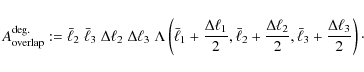
As is evident from Fig. 2, center panel, the relative deviation of (13) from the true overlap area is still fairly small, but - unsurprisingly - noticeably stronger than for (12). The right-hand panel gives the size of the overlap area for values of
Thus, we suggest to incorporate degenerate triangle configurations into our formalism by replacing
![]() in all arguments of
in all arguments of ![]() for
these cases. This way, we heuristically correct for the breakdown of
approximations in the assignment of the actual area, over which
triangle configurations are averaged. While the modification is at this
stage only motivated by the geometrical interpretation, we will
establish a more strict foundation of (13) by relating it to Wigner symbols in Sect. 5.1.
for
these cases. This way, we heuristically correct for the breakdown of
approximations in the assignment of the actual area, over which
triangle configurations are averaged. While the modification is at this
stage only motivated by the geometrical interpretation, we will
establish a more strict foundation of (13) by relating it to Wigner symbols in Sect. 5.1.
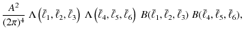
4 Bispectrum covariance
The covariance of the bispectrum is defined as
The computation of the correlator of two bispectrum estimators involves a 6-point correlator of g, which can be expanded into its connected parts as e.g. outlined in Bernardeau et al. (2002a). Denoting the connected correlators by a subscript c, which will only be done in this paragraph to avoid confusion, we obtain
where the permutations are to be taken with respect to the indices of the angular frequencies such that for each correlator, no combination of indices is repeated (as the individual correlators are invariant under permutations of the indices within that correlator). The resulting connected parts are related to spectra via
where we identify
Introducing a shorthand notation
![]() ,
one can write the correlator of the bispectrum estimators by using (3) as
,
one can write the correlator of the bispectrum estimators by using (3) as
which then allows us to insert (15) and (16). The resulting terms contain products of several delta-distribution. Concerning the terms containing three two-point correlators, one obtains e.g.
and likewise for all other terms in which the correlators do not contain one angular frequency each out of the sets
To proceed, we demonstrate the treatment of some exemplary terms in the covariance, for instance
where the integrations over
where we again pulled
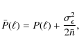
for convenience. By making use of (2) and defining the bin-averaged power spectrum as
see Joachimi et al. (2008), in analogy to the definition of the bin-averaged bispectrum, one obtains the expression
Terms composed of two three-point correlators can be processed as follows,
where to generate the Kronecker symbol
which, after inserting this expression into (17), cancels the product
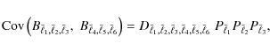
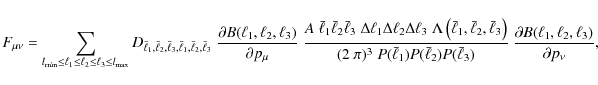
Combining these results, we obtain the total bispectrum covariance
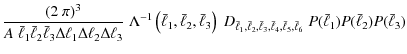
where the prefactor reads
The general form of the covariance terms is in agreement with the expressions derived in Sefusatti et al. (2006). As mentioned in Sect. 2, shot or shape noise can readily be included into this covariance by adding a corresponding noise term to the power spectra. Weak lensing or galaxy clustering surveys often have in addition tomographic information, so that the data is binned into (photometric) redshift bins. The covariance can be generalized to this case in a straightforward manner by obeying the practical rule that each photometric redshift ``sticks'' to the angular frequency it is assigned to, see Takada & Jain (2004). A similar argument holds for the generalization to CMB polarization bispectrum covariances (Hu 2000).
5 Equivalence to spherical harmonics approach
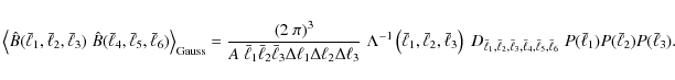
In this section we demonstrate that both our and the spherical harmonic approach are equivalent in the sense that they measure the same information in a survey. Moreover, we investigate the behavior with respect to parity, and the relation between the covariances of both approaches, considering for the remainder of this work only the Gaussian part of (26).
5.1 Comparison of covariances
On the celestial sphere one can decompose the random field g into spherical harmonics, which produces a set of coefficients
![]() with
with ![]() integers and
integers and
![]() ,
,
![]() .
In terms of the
.
In terms of the
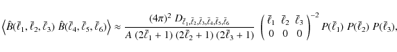
![]() one can define a bispectrum estimator as (e.g. Hu 2000)
one can define a bispectrum estimator as (e.g. Hu 2000)
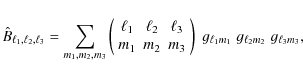
where the object in parentheses is the Wigner-3j symbol. Properties of the Wigner symbol are reviewed in Hu (2000); most importantly, it obeys the triangle condition, i.e. it is non-zero only for
where
valid for
where still the angular frequencies are required to be integer, and L even. As is true for our approach, (30) holds for
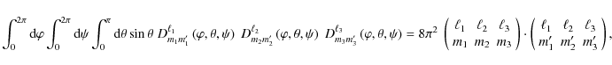
When comparing the spherical harmonics and the Fourier-plane approach, Hu (2000) already came across integrals of the form (6). We reproduce his computation,


where
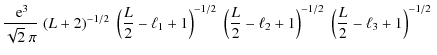
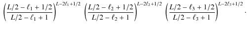
To allow for a comparison between (31) and our approach based on (6), we need to establish a relation between the square of the Wigner symbol and (8). We refer to Borodin et al. (1978, see also references therein)
who compute approximation formulae of the Wigner symbol in the context
of the quasi-continuous limit of quantum states with high angular
momenta. The base of their derivation is formed by the exact relation
where

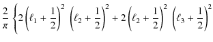
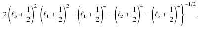
which allows us to generalize the Wigner symbol to real-valued arguments. Equation (33) holds only for
![\begin{figure}
\par\includegraphics[scale=.61,angle=270]{12906fg4.ps}
\end{figure}](/articles/aa/full_html/2009/48/aa12906-09/img168.png)
|
Figure 4:
Fractional error of the approximation formulae for the Wigner symbol. Left panel: shown are the relative deviations of (33) and (34) from the true absolute value of the Wigner symbol. The same triangle configurations as in Fig. 2 are used. Results for
|
| Open with DEXTER | |
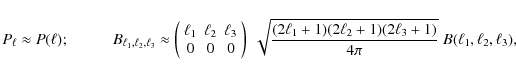
As is demonstrated in Fig. 4, we find that (33) constitutes an excellent approximation, whose accuracy over a wide range of ![]() -values is orders of magnitude better than the approximation given in Takada & Jain (2004), Eq. (A3),
-values is orders of magnitude better than the approximation given in Takada & Jain (2004), Eq. (A3),
Only for triangle configurations close to degeneracy does the latter formula perform slightly better. Both approximation formulae are least accurate in the case of a degenerate triangle configuration with fractional errors around 10% or slightly above, but improve quickly to very small percentage deviations when the configuration approaches a more equilateral form. In Fig. 4 we also plot the fractional errors as a function of the triangle area enclosed by the three angular frequency vectors and as a function of the internal angle
For
![]() ,
and if the triangle configuration is not too close to the degenerate case, one may approximate
,
and if the triangle configuration is not too close to the degenerate case, one may approximate
![]() ,
so that one finds from (8) and (33)
,
so that one finds from (8) and (33)
Remarkably, since for integer angular frequencies we have
Inserting (35) into (30), and using
![]() for
for
![]() ,
we get
,
we get
which is equivalent to (23) if the latter equation is specified to
5.2 Parity
To elucidate the different noise properties of the Fourier-plane and spherical harmonic bispectrum estimators, we investigate their behavior with respect to parity. In two dimensions the parity transformation corresponds to an axis reflection, or equivalently, the reversal of the polar angle of all spatial vectors. To flip the parity of a triangle, one can do an odd permutation of its sides, see e.g. the two triangles sketched in Fig. 1. Hence, to test the behavior of estimators for triangles of different parity, it is sufficient to flip any two of its angular frequency arguments.
Consulting (27), we find

because of the behavior of the Wigner symbol under change of parity,
and likewise for all odd permutations of the columns in the Wigner symbol. Thus, the spherical harmonics estimator is parity-invariant for L even and changes sign for L odd. Most cosmological theories predict parity-invariant large-scale structures and CMB anisotropies. If parity symmetry is built into the cosmological model at consideration, measures that vary under parity transformations do not have any predictive power, wherefore they are usually not considered in a data analysis. Accordingly, (27) is only used for arguments that have L even. Note that parity invariance is also incorporated into the relation between the spherical harmonics and Fourier-plane bispectra, see the second equality of (29), via the Wigner symbol which vanishes for L odd (this behavior is a direct consequence of (38) for m1=m2=m3=0).
The Fourier-plane estimator is by design parity-invariant, which can be seen mathematically from swapping arguments of (3), or illustratively by inspecting Fig. 1.
From the sketch it is evident that triangle configurations of different
parity are averaged over with equal weight. For a more formal argument,
we can explicitly construct estimators that average only over triangle
configurations of the same parity. To this end, consider the
two-dimensional cross product
![]() (Schneider & Lombardi 2003) of the angular frequency vectors
(Schneider & Lombardi 2003) of the angular frequency vectors
![]() .
If they form a triangle, one finds
.
If they form a triangle, one finds
![]() ,
which follows from
,
which follows from
![]() .
A change in the parity of the triangle implies a sign flip in these cross products.
.
A change in the parity of the triangle implies a sign flip in these cross products.
Noting that
![]() ,
we compute a condition on the polar angles,
,
we compute a condition on the polar angles,
To obtain the parity transformed triangle, swap the signs of the polar angles in (39). Under the premise that the vectors do form a triangle, one of the conditions in (39) is redundant, the remaining ones restricting the angular integrations in the averaging of (3). For instance, the integration ranges could be modified to
which we use to define the following bispectrum estimators,


Here, we have symmetrized the restricted integrations (40) by averaging over all either even or odd permutations of
Note that the prefactor of the estimators in (41) is diminished by a factor of 2 with respect to (3), which is necessary to keep them unbiased. This can be shown by computing the expectation value of (41) in close analogy to the procedure outlined in Sect. 2. However, the separate consideration of angular and radial integrals that enabled us to make use of (6) is not possible anymore in this non-symmetric case. For instance, given fixed
![]() ,
the restricted angular integrations (40) can still produce a triangle of opposite parity by including a triangle with
,
the restricted angular integrations (40) can still produce a triangle of opposite parity by including a triangle with
![]() and
and
![]() .
This is reflected in the fact that the integration (6), if properly normalized
.
This is reflected in the fact that the integration (6), if properly normalized![]() , still yields the same result when limiting the length of the integration range to
, still yields the same result when limiting the length of the integration range to ![]() .
.
Instead, one can execute the integral over the angular frequency which
is still averaged over the full two-dimensional plane, such as

where

Comparing this result to (4), the estimators (41) have indeed to be smaller by a factor of 2 to still be unbiased.
To obtain bispectrum estimators that are completely analogous to (27), we define
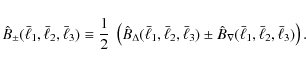
As
With (44)
at hand, one can readily extract the different treatment of even and
odd parity measures in the spherical harmonic and Fourier-plane
formalisms. Estimators (27) separate the set of possible arguments
![]() disjointly into parity even (L even) and parity odd (L odd), whereas
disjointly into parity even (L even) and parity odd (L odd), whereas ![]() and
and ![]() are defined on the same full set of angular frequency combinations
are defined on the same full set of angular frequency combinations![]() . In other words, when limiting
. In other words, when limiting ![]() to integer angular frequencies only, the same information is contained
in ``half'' the number of measures in the spherical harmonics case,
namely those with L even. The latter estimators have a covariance of half the size of the covariance of
to integer angular frequencies only, the same information is contained
in ``half'' the number of measures in the spherical harmonics case,
namely those with L even. The latter estimators have a covariance of half the size of the covariance of ![]() ,
so that the overall information content is the same for both approaches - as required.
,
so that the overall information content is the same for both approaches - as required.
5.3 Information content
We verify the findings of the foregoing section by comparing the
information contained in both approaches in terms of the Fisher matrix (Tegmark et al. 1997). For a practical implementation we specialize to a non-tomographic weak lensing survey (see e.g. Bartelmann & Schneider 2001,
for an overview), assuming a cosmology-independent covariance that is
well approximated by the Gaussian approximation, i.e. using (23) and (30), respectively. To allow for direct comparison, we limit the Fourier-plane approach to integer ![]() with all bin sizes set to unity. Due to the symmetry under permutations
of the arguments of the bispectra, one can impose the condition
with all bin sizes set to unity. Due to the symmetry under permutations
of the arguments of the bispectra, one can impose the condition
![]() on both formalisms, rendering a block-wise diagonal covariance matrix. Inspecting (23), the only dependence on the arguments of the second bispectrum, i.e.
on both formalisms, rendering a block-wise diagonal covariance matrix. Inspecting (23), the only dependence on the arguments of the second bispectrum, i.e. ![]() to
to ![]() ,
is due to the Kronecker symbols (21), so that the summations over
,
is due to the Kronecker symbols (21), so that the summations over ![]() to
to ![]() become trivial.
become trivial.
Hence, the Fisher matrix can be written as
where
Weak lensing power spectra are computed for a standard ![]() CDM cosmology, including non-linear evolution via the fit formula of Smith et al. (2003). The bispectra are obtained via perturbation theory (e.g. Fry 1984), using Scoccimarro & Couchman (2001) with the definition of the non-linear wave vector by Takada & Jain (2004)
to account for non-linear evolution. For the projections along the line
of sight we assume a redshift probability distribution according to Smail et al. (1994) with
CDM cosmology, including non-linear evolution via the fit formula of Smith et al. (2003). The bispectra are obtained via perturbation theory (e.g. Fry 1984), using Scoccimarro & Couchman (2001) with the definition of the non-linear wave vector by Takada & Jain (2004)
to account for non-linear evolution. For the projections along the line
of sight we assume a redshift probability distribution according to Smail et al. (1994) with ![]() and a deep survey of 0.9 median redshift. Shape noise is incorporated by replacing the power spectra in the covariances with
and a deep survey of 0.9 median redshift. Shape noise is incorporated by replacing the power spectra in the covariances with
where the ellipticity dispersion
| Figure 5:
Comparison of the Fisher information as obtained by spherical harmonics
and Fourier-plane approach. Given is the relative deviation r as a function of the maximum angular frequency
|
|
| Open with DEXTER | |
We calculate the relative deviation of the Fisher information,
![]() ,
as a function of
,
as a function of
![]() .
Note that, since we only consider ratios of F, the survey size A drops out. Our results are shown in Fig. 5. For
.
Note that, since we only consider ratios of F, the survey size A drops out. Our results are shown in Fig. 5. For
![]() very close to
very close to
![]() one sees alternating jumps in r which can mostly be traced back to the fact that, due to the condition
one sees alternating jumps in r which can mostly be traced back to the fact that, due to the condition
![]() ,
the terms entering (45) do not always split exactly half into L even and odd. After this ``burn in'' for
,
the terms entering (45) do not always split exactly half into L even and odd. After this ``burn in'' for
![]() ,
r shows only little variation. The remaining offset from zero,
which is slowly decreasing, can entirely be assigned to the different
prefactors in the covariances, i.e. the terms related to the Wigner
symbol and
,
r shows only little variation. The remaining offset from zero,
which is slowly decreasing, can entirely be assigned to the different
prefactors in the covariances, i.e. the terms related to the Wigner
symbol and ![]() ,
respectively. The range of angular frequencies plotted in Fig. 5 is still far from any physically relevant situation, but nonetheless the two approaches agree already better than 99%.
,
respectively. The range of angular frequencies plotted in Fig. 5 is still far from any physically relevant situation, but nonetheless the two approaches agree already better than 99%.
6 Conclusions
In this work we intended to give insight into the derivation and the form of the bispectrum covariance in the flat-sky approximation, based exclusively on the two-dimensional Fourier formalism. We defined an unbiased estimator that takes the average over the overlap of annuli in Fourier space, and computed its covariance. To obtain precise normalizations, a case distinction is necessary between degenerate and non-degenerate triangle configurations. However, given that both normalizations become very similar for

This formula is readily generalized to the total covariance by modifying the arguments of
While the general form of our result was in agreement with existing work, we found, contrary to Hu (2000),
that the size of the covariance is a factor of 2 larger than the one
obtained by the flat-sky spherical harmonic approach. By defining
parity-sensitive bispectrum estimators, we discussed the behavior of
both formalisms with respect to parity transformations, arguing that
the difference in the covariances is indeed to be expected because in
the spherical harmonic framework, parity-invariant measures are
restricted to a subset of the angular frequency combinations at which
the bispectra are evaluated. In a practical example we demonstrated
that both approaches indeed contain the same information in terms of
the Fisher matrix, with a high level of agreement. As a consequence, we
can confirm that studies performed in the flat-sky spherical harmonic
approach, such as Takada & Jain (2004), yield correct parameter constraints as long as the analysis is restricted to integer ![]() with the sum of the three angular frequencies being even.
with the sum of the three angular frequencies being even.
We established a relation between the geometrical and intuitive process of averaging over the overlapping regions of annuli in the Fourier plane and the Wigner symbol of the spherical harmonic approach. Both quantities were demonstrated to be in turn connected to a simple measure that is proportional to the size of the area enclosed by the triangle configuration for which the bispectrum is calculated. This resulted in convenient, yet precise approximation formulae for the prefactors of the covariances of both approaches at consideration.
Under the assumption of a compact survey geometry and scales much smaller than the extent of the survey area, (26) provides a cleanly derived bispectrum covariance matrix that naturally incorporates the scaling with survey size, is not restricted to integer angular frequencies, and allows for any appropriate binning.
AcknowledgementsThe authors would like to thank Bhuvnesh Jain and Masahiro Takada for helpful discussions and the referee for a helpful report. We thank Joel Bergé for comparison tests of our bispectrum codes. B.J. is grateful to Sarah Bridle for kind hospitality at UCL. B.J. acknowledges support by the Deutsche Telekom Stiftung and the Bonn-Cologne Graduate School of Physics and Astronomy. X.S. is supported by the International Max Planck Research School (IMPRS) for Astronomy and Astrophysics. This work was supported by the DFG under the Priority Programme 1177 Galaxy Evolution and within the Transregional Collaborative Research Centre TR33 The Dark Universe.
References
- Bartelmann, M., & Schneider, P. 2001, Phys. Rep., 340, 291 [NASA ADS] [CrossRef]
- Bernardeau, F., Colombi, S., Gaztañaga, E., et al. 2002a, Phys. Rep., 367, 1 [NASA ADS] [CrossRef]
- Bernardeau, F., Mellier, Y., & van Waerbeke, L. 2002b, A&A, 389, L28 [NASA ADS] [EDP Sciences] [CrossRef]
- Borodin, K., Kroshilin, A., & Tolmachev, V. 1978, TMF, 34, 110
- Cooray, A., Sarkar, D., & Serra, P. 2008, Phys. Rev. D, 77, 123006 [NASA ADS] [CrossRef]
- Fry, J. 1984, ApJ, 279, 449 [NASA ADS] [CrossRef]
- Gradshteyn, I., Ryzhik, I., Jeffrey, A., et al. 2000, Tables of Integrals, Series, and Products (Academic Press)
- Hu, W. 1999, ApJ, 522, 21 [NASA ADS] [CrossRef]
- Hu, W. 2000, Phys. Rev. D, D62, 043007 [NASA ADS] [CrossRef]
- Jarvis, M., Bernstein, G., & Jain, B. 2004, MNRAS, 352, 338 [NASA ADS] [CrossRef]
- Joachimi, B., Schneider, P., & Eifler, T. 2008, A&A, 477, 43 [NASA ADS] [EDP Sciences] [CrossRef]
- Kaiser, N. 1998, ApJ, 498, 26 [NASA ADS] [CrossRef]
- Matarrese, S., Verde, L., & Heavens, A. 1997, MNRAS, 290, 651 [NASA ADS]
- Schneider, P., & Lombardi, M. 2003, A&A, 397, 809 [NASA ADS] [EDP Sciences] [CrossRef]
- Scoccimarro, R. 2000, ApJ, 544, 597 [NASA ADS] [CrossRef]
- Scoccimarro, R., & Couchman, H. 2001, MNRAS, 325, 1312 [NASA ADS] [CrossRef]
- Scoccimarro, R., Feldman, H., Fry, J., et al. 2001, ApJ, 546, 652 [NASA ADS] [CrossRef]
- Sefusatti, E., Crocce, M., Pueblas, S., et al. 2006, Phys. Rev. D, 74, 023522 [NASA ADS] [CrossRef]
- Smail, I., Ellis, R., & Fitchett, M. 1994, MNRAS, 270, 245 [NASA ADS]
- Smith, R., Peacock, J., Jenkins, A., et al. 2003, MNRAS, 341, 1311 [NASA ADS] [CrossRef]
- Takada, M., & Jain, B. 2004, MNRAS, 348, 897 [NASA ADS] [CrossRef]
- Tegmark, M., Taylor, A., & Heavens, A. 1997, ApJ, 480, 22 [NASA ADS] [CrossRef]
Footnotes
- ... normalized
![[*]](/icons/foot_motif.png)
- In the derivation of Sect. 2 the proper normalization of
 for each angular integral is hidden within
  .
Note that we have given (6) without this normalization, whereas it is included in (11).
.
Note that we have given (6) without this normalization, whereas it is included in (11).
- ... combinations
- A similar behavior as for the spherical harmonic estimators would have been unexpected since the possible arguments of
 form a non-countable set.
All Figures
|
|
Figure 1:
Sketch of the annuli and their overlap for fixed
|
| Open with DEXTER | |
| In the text | |
|
|
Figure 2:
Comparison of expressions for the overlap area of annuli. Left panel: relative deviation of (12) from the overlap area of the annuli as a function of angular frequency. The bin width is kept constant at
|
| Open with DEXTER | |
| In the text | |
|
|
Figure 3:
Sketch of the region averaged over in case of a degenerate triangle, again for fixed
|
| Open with DEXTER | |
| In the text | |
|
|
Figure 4:
Fractional error of the approximation formulae for the Wigner symbol. Left panel: shown are the relative deviations of (33) and (34) from the true absolute value of the Wigner symbol. The same triangle configurations as in Fig. 2 are used. Results for
|
| Open with DEXTER | |
| In the text | |
| |
Figure 5:
Comparison of the Fisher information as obtained by spherical harmonics
and Fourier-plane approach. Given is the relative deviation r as a function of the maximum angular frequency
|
| Open with DEXTER | |
| In the text | |
Copyright ESO 2009
Current usage metrics show cumulative count of Article Views (full-text article views including HTML views, PDF and ePub downloads, according to the available data) and Abstracts Views on Vision4Press platform.
Data correspond to usage on the plateform after 2015. The current usage metrics is available 48-96 hours after online publication and is updated daily on week days.
Initial download of the metrics may take a while.