On the eccentricity of self-gravitating circumstellar disks in eccentric binary systems

F. Marzari; H. Scholl; P. Thébault; C. Baruteau

doi:10.1051/0004-6361/200912251

Home

All issues

Volume 508 / No 3 (December IV 2009)

A&A, 508 3 (2009) 1493-1502

Full HTML

Free Access

Issue		A&A Volume 508, Number 3, December IV 2009


Page(s)		1493 - 1502
Section		Planets and planetary systems
DOI		https://doi.org/10.1051/0004-6361/200912251
Published online		01 October 2009

A&A 508, 1493-1502 (2009)

On the eccentricity of self-gravitating circumstellar disks in eccentric binary systems

F. Marzari¹ - H. Scholl² - P. Thébault³ - C. Baruteau⁴

1 - Dipartimento di Fisica, University of Padova, Via Marzolo 8, 35131 Padova, Italy
2 - Laboratoire Cassiopée, Université de Nice Sophia Antipolis, CNRS, Observatoire de la Côte d'Azur, BP 4229, 06304 Nice Cedex, France
3 - Observatoire de Paris, Section de Meudon, 92195 Meudon Principal Cedex, France
4 - Astronomy and Astrophysics Department, University of California, Santa Cruz, CA 95064, USA

Received 1 April 2009 / Accepted 3 August 2009

Abstract
Aims. We study the evolution of circumstellar massive disks around the primary star of a binary system focusing on the computation of disk eccentricity. In particular, we concentrate on its dependence on the binary eccentricity. Self-gravitation is included in our numerical simulations. Our standard model assumes a semimajor axis for the binary of 30 AU, the most probable value according to the present binary statistics.
Methods. Two-dimensional hydrodynamical computations are performed with FARGO. Besides the dynamical standard method to determine disk eccentricities, we apply a morphological method which may allow a better comparison with observations.
Results. Self-gravitation leads to disks that, on average, have low eccentricity. Moreover, the orientation of the disk computed with the standard dynamical method always librates instead of circulating as in simulations without self-gravitation. The disk eccentricity decreases with the binary eccentricity, a result found also in models without self-gravitation.
Conclusions. Disk self-gravitation appears to be an important factor in determining the evolution of a massive disk in a binary system. High eccentricity binaries are not necessarily a hostile environment for planetary accretion.

Key words: planetary systems: formation - planetary systems: protoplanetary disks - methods: numerical

1 Introduction

All stages of planet formation in binary star systems might be strongly influenced by the characteristic gravitational field. (Thébault et al. 2004,2006; Quintana et al. 2002; Marzari & Scholl 2000; Paardekooper et al. 2008; Thébault et al. 2008). The protoplanetary disk around a primary star, for instance, is perturbed by the companion affecting its morphology and dynamical structure. Spiral waves develop at major resonances in the disk. Its shape is expected to be elliptic with varying eccentricity (Kley et al. 2008; Kley & Nelson 2008; Paardekooper et al. 2008). Both these features may alter the dust sedimentation process on the mid plane of the disk and the grain accumulation into planetesimals which might even be inhibited (Nelson 2000). More eccentric trajectories of the grains, dragged by the gas, increase the impact rate but, on the other hand, might lead to destructive collisions by increasing the relative velocity. A more turbulent disk might, however, favor accumulation of dust in bigger bodies due to gravitational instability on a faster timescale.

Understanding the morphology of circumprimary gas disks is also crucial for the subsequent phase of planetesimal accumulation. Indeed, several recent studies have shown that this stage might be severely hampered, or even stopped by the combination of secular perturbations from the companion star and friction with gas (Xie & Zhou 2008; Thébault et al. 2009,2006,2008). This combined effect forces a differential phasing of planetesimal orbits according to sizes, which leads to high impact velocities for a large fraction of planetesimal-planetesimal collisions, which could in some cases lead to an accretion-hostile dynamical environment. Paardekooper et al. (2008) have shown that these results, obtained assuming static axisymmetric gas disks, could be further amplified when letting the gas disk evolve and ``feel'' the binary perturbations. The most accretion-hostile cases were obtained when the gaseous disk reached high eccentricities, with impact velocities almost twice as high as in the axisymmetric case, while low eccentricity disks gave results similar to that with a static disk There is in principle a possibily for an eccentric gas disc to lead to lower drag effects, that is, if this eccentricity is close to the forced secular eccentricity of the planetesimals (see Eq. (17) of Paardekooper et al. 2008). However, this theoretical behaviour is only possible for a very specific radial profile of the gas disk density and has never been observed in test simulations, indicating that this case is probably only a marginal possibility (see detailed discussion in Sect. 6.1 of Paardekooper et al. 2008).

Also, the alternative formation mechanism for giant planets by rapid disk gravitational instability seems to be affected by the companion perturbations. According to Boss (2006), the presence of the secondary star might induce planet formation, even if his results are questioned in Mayer et al. (2006).

Before performing time consuming simulations of planetesimal accretion in a binary system with a hybrid code like, for instance, in Kley & Nelson (2007), Paardekooper et al. (2008) and Marzari et al. (2008), we first investigate the disk evolution depending on the parameters of the system. This paper is devoted to the influence of the binary eccentricity and self-gravitation on the disk structure.

In addition, the eccentricity of circumstellar disks in binaries may also become an observable feature in the future. The next generation of interferometers (like ALMA, Atacama Large Millimeter/submillimeter Array) aiming to obtain high angular resolution millimeter and sub-millimeter images, might resolve the molecular gas and dust components of disks by deriving values for the disk size and ellipticity. Lim and Takakuwa (2006) have already performed imaging of the dusty disks with VLA (Very Large Array) in the L1551 IRS 5 binary system with a resolution of about 5 AU while with ALMA it might be possible to gain a factor of from 2 to 5. The morphology of protostellar disks might be derived by a comparison with numerical simulations. The matching of observable features will allow us to derive important constraints on physical disk parameters. An important parameter in comparing observations and simulations is the eccentricity of the disk. Classical image treatment methods developed to measure the eccentricity and orientation of elliptical galaxies, once applied to circumstellar disks, may yield different values compared to those usually obtained by numerical simulations. We will discuss this problem in Sect. 2.

Investigating the effect of a stellar companion on the evolution of a disk surrounding the primary necessitates the exploration of a very large parameter space determined in particular by physical parameters for the disk and orbital parameters of the binary system. In a first step, we focus on the influence of the binary eccentricity using for all other parameters mean standard values which are expected from observations. For the simulations, we use the latest release of the hydrodynamical code FARGO (Masset 2000) which now includes disk self-gravitation (Baruteau & Masset 2008). Comparison with former simulations allows the investigation of its influence on the formation of structures in the disk, on its eccentricity and orientation.

The paper is structured in the following way. We first compare in Sect. 2 the standard way to derive the disk eccentricity in a simulation with image treatment methods developed for observed disks. In Sect. 3 we recall the numerical FARGO model and give the parameters of our simulated systems. Section 4 is devoted to the importance of self-gravitation on the evolution of a disk. Section 5 is focused on the dependence of disk evolution on binary eccentricity. In Sect. 6 we summarize and discuss our results.

2 Dynamical and morphological disk eccentricities

Under the perturbations of the binary companion, the disk around the primary star modifies its shape. The three major perturbing forces acting on each gas particle, which are the gravitational attraction exerted by the companion star, the gas pressure and the gravitational attraction by the disk, act in synergy and modify the trajectories of each individual gas particle. In a disk surrounding an isolated single star, trajectories are in a first approximation nearly circular when the self-gravitation of the disk is neglected. The gravitational potential due to the disk and the companion star modify the trajectories which can be approximated by elliptical trajectories with varying eccentricities. Hydrodynamical simulations of a disk yield for each cell of the grid the velocity of the gas that can be used to compute an individual eccentricity attributed to each cell. The mass-weighted average of the eccentricities of all cells has been used as an estimator for the eccentricity of the disk (Kley et al. 2008; Pierens & Nelson 2007; Paardekooper et al. 2008). We call it in the following the dynamical disk eccentricity $e_{\rm d}$ . It is defined by:

$\begin{displaymath}e_{\rm d} = \frac{ \sum_i e_i m_i} {M_{\rm d}} \end{displaymath}$

(1)

where e_i is the eccentricity of each cell i of the grid, assuming that the local position and velocity vectors uniquely define a 2-body Keplerian orbit, while m_i is its mass computed from the local disk density. $M_{\rm d}$ is the disk mass. In a similar way, a mass averaged perihelion of the disk $\varpi _{\rm d}$ with respect to the orientation of the binary's apsidal line can be computed. We call these the dynamical elliptical elements of the disk.

If the self-gravitation of the disk is included in the model, the calculation of e_i and $\varpi _i$ must be improved. When a two-body Keplerian orbit is derived for each gas cell it must account for the gravitational attraction of all the other disk components. An approximate perturbative model can be used in this case as in Marzari et al. (2008). The disk is approximated as a sequence of uniform density rings starting from the inner radius outwards until the outer border of the disk is reached. The density of each ring is calculated by averaging the local disk density within the ring derived from the numerical simulation. The gravitational attraction of each ring on each individual gas cell can be analytically computed (Krogh et al. 1982) and, being a radial force, it can be added to the central force of the star. A Keplerian orbit for each gas cell is computed by adopting a slightly increased mass for the star which must be updated at each timestep since the mass distribution within the disk changes because of spiral waves and disk eccentricity.

By comparing the computation of the orbital elements of each disk component with and without the abovementioned algorithm to account for self-gravitation we find that for eccentricities greater than 0.1 the discrepancy between a rough 2-body estimate of e_i and $\varpi _i$ derived with a constant stellar mass and that obtained with a varying stellar mass because of the disk self-gravitation are not very different; thus we neglect this effect in this paper. We can also safely neglect the effects of pressure forces in a first approximation since they do not introduce a large error in the computation of a reliable value of both e_i and $\varpi _i$ . In conclusion, hereinafter we compute the eccentricity e_i of each disk component by using a 2-body approximation with fixed stellar mass.

An important question is how to relate $e_{\rm d}$ to the disk eccentricity an observer would obtain applying an image treatment method. Eccentricities of elliptically shaped objects, in particular of elliptical galaxies, on a digitized image are obtained basically by two classical methods. One method uses all pixels that form an object. Computing first and second order momenta of the object yields eccentricity, semimajor axis and orientation of an ellipse approximating the object. The second method uses contour lines formed by pixels with about the same intensity. An ellipse is then fitted to the contour line. We applied the second method, which is implemented in MATLAB, where we force the focus of the ellipse to lie on the star. This method yields the $\it morphological$ parameters $e_{\rm m}$ , $\varpi _{\rm m}$ and $a_{\rm m}$ of a disk. Figure 1 illustrates the morphological method. Using the gas densities at each cell in a simulation, we produce a synthetic CCD image. The pixel values correspond to gas densities. The morphological parameters depend on the choice of the intensity values of pixels and, hence, of a gas density value $\rho _0$ forming the contour line which corresponds to the border of the disk.

$\begin{figure} \par\resizebox{9cm}{!}{\includegraphics{fig1.eps}} \end{figure}$	Figure 1: Example of outer disk contour identification by MATLAB. The value of $\rho _0$ is set to 10^-6. An ellipse is then fitted to the contour to compute $e_{\rm m}$ , $\varpi _{\rm m}$ and $a_{\rm m}$ . The color scaling gives the logarithm of the gas density in normalized units.
Open with DEXTER

The advantages of using morphological parameters are the following:

they are independent of the internal structure of the disk;
they are close to observable quantitiest;
the morphological semimajor axis $a_{\rm m}$ can be used as a reliable estimate of the disk size.

It is noteworthy that the value $e_{\rm m}$ may significantly differ from the average value of the e_is computed for $a = a_{\rm m}$ because at the outer border of the disk the distribution of the e_is and $\varpi _i$ s is sparse. In Fig. 2 we show the distribution of both e_i and $\varpi _i$ as a function of the cell semimajor axis a_i. Close to the star the values of $\varpi _i$ are very similar, independently of the azimuthal angle. However, at the outer border the distribution broadens and the values e_i and $\varpi _i$ depend on the azimuthal angle. In the bottom plot we show a case in which the values of $\varpi _i$ are distributed in the range $[0,2\pi]$ . For this reason $e_{\rm m}$ may be significantly different to $\langle e_i (a_{\rm m})\rangle$ .

The morphological method to compute disk eccentricities depends on the choice of $\rho _0$ , which is not an objective selection criterium. This is, however, a very common problem for observers applying image treatment methods. In addition, in our simulations we find that the border of the disk is always well defined and it drops to small values very quickly due to the tidal perturbations of the star. This is shown in Fig. 3 where at about 8 AU from the central star the disk density rapidly drops. This makes us confident that the method to compute the overall disk eccentricity $e_{\rm m}$ and its orientation $\varpi _{\rm m}$ is not very sensitive to the minimum density value selected in the computations when this is below 10^-6 (obtained after exploring a significant numer of test cases), which will be the value of $\rho _0$ always adopted in this paper. A test computation of $e_{\rm m}$ for different values of $\rho _0$ ranging from 10^-5 to 10^-7 gave a maximum variation of less than 7%.

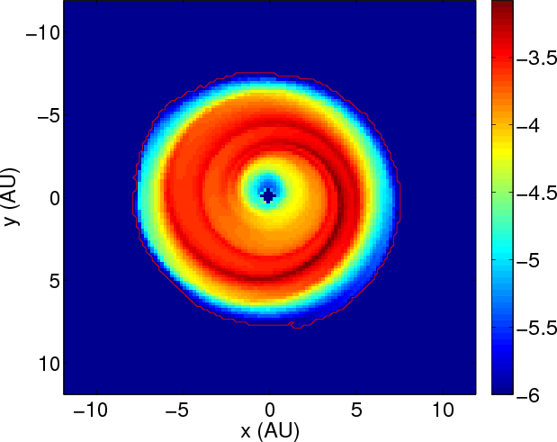
The drastic truncation of the disk (see Fig. 3) makes us also confident that the shape derived from the morphological analysis might be retrieved in the future from observations even if the disk is optically thick. The shape of an optically thin disk can be retrieved by observations in the millimeter range and the column density (our model superficial density) is indeed proportional to the flux. For optically thick disks this is not necessarely true, however the sharp truncation of the disk might be retrieved by inspecting the scattered light from the star.

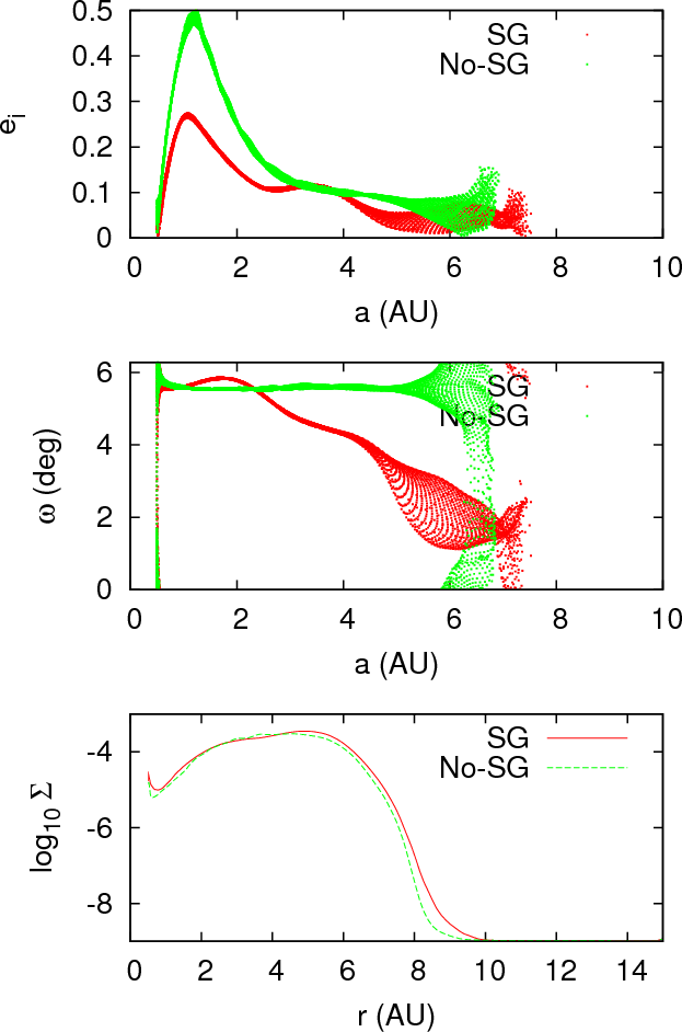
$\begin{figure} \par\resizebox{9cm}{!}{\includegraphics{em_tre.eps}} \end{figure}$	Figure 2: Distribution of e_i ( top plot) and $\varpi _i$ ( middle plot) over the disk as a function of a_i for both the SG and non-SG cases. In the bottom plot the density distribution averaged over the sectors is shown.
Open with DEXTER

3 Numerical set up

3.1 The hydrodynamical model

To model the evolution of the disk we use the hydrodynamical code FARGO (Masset 2000) solving the Navier-Stokes and continuity equations on a 2-dimensional polar grid. The mesh center lies at the primary and the indirect terms are included in the potential calculation. Since we are not interested in the evolution of the binary star system but only in the structure of the disk under the binary perturbation after the tidal truncation of the disk, we fix the orbital parameters of the companion star. In the latest release of FARGO a Poisson equation solver based on the Fourier method has been implemented (Baruteau & Masset 2008) allowing us to properly model the disk self-gravitation (hereinafter SG). The impact of SG on the disk evolution is relevant when modelling highly perturbed massive disks.

In all the simulations we use a grid extending from 0.5 to 15 AU from the primary star: the number of rings is 256 while that of the sectors is 512. The aspect ratio h = H/r is constant all over the disk and set to 0.05. The initial density profile declines as $\Sigma = \Sigma_0 r^{-1/2}$ and is smoothly Gaussian truncated at the inner and outer borders. At the inner border $\Sigma$ is reduced by a factor of 10 betwen 0.55 and 0.5 AU, while at the outer border of the disk, starting from 11 AU, the density is decreased to $\Sigma_f = 10^{-9}$ within 2 AU. Following Kley et al. (2008), to prevent numerical instabilities at the outer border of the disk caused by very low density values, we introduce a density floor equal to $\Sigma_f$ . Whenever the evolution leads to a density value lower than $\Sigma_f$ , $\Sigma$ is reset to $\Sigma_f$ . In a series of tests this has proven to be a good value preventing instabilities and not leading to an artificial mass growth of the disk.

We adopt a density at 1 AU equal to 2.5e-4 in normalized units, giving an initial mass of the disk equal to $0.04 ~M_{\rm sun}$ . Our disk is more massive than that studied in Kley & Nelson (2008) whose total mass was about $0.0015~ M_{\rm sun}$ . Since the results do not scale only with the size of the system but also with the mass of the disk, we expect that the results can be different.

We used a non-reflecting boundary condition in all our calculations. It is aimed at removing as many reflections as possible off the grid boundaries, while allowing mass to flow through the inner and outer edges. Kley & Nelson (2008) used a different kind of boundary condition to model the disk in $\gamma$ Cephei forcing a viscous inwards flow of a disk at equilibrium at the inner border. With the non-reflecting boundary condition we have a mass inwards-flow which is comparable to that computed by Kley & Nelson (2008) in terms of the mass fraction of the disk and we do not observe any strong outflow of disk material during the periastron phase through the inner border. A small elliptic central hole in the disk develops with time (see Fig. 1), a consequence of the eccentric orbits of the gas in the proximity of the star. Since our grid extends down to 0.5 AU, all gas particles with pericenter q lower than 0.5 AU are expected to exit the inner border of the disk. Due to the collimated values of the perihelia $\varpi$ the outflow of the particles with q < 0.5 AU creates a region of low density with an elliptical shape centered on the star (see Appendix A). If the $\varpi _i$ s were random, then the inner hole would have been circular with a radius greater than 0.5. In support of this interpretation, we find that the size of the elliptic hole in the simulations is well reproduced by modelling its outer shape with a Keplerian orbit with the pericenter at 0.5 AU and with an eccentricity equal to the average eccentricity e_i of the local gas cells. In conclusion, with our boundary condition, the code produces reasonable results taking into account the truncation of the disk at the inner edge. Of course, setting the inner rim of the disk to 0.5 AU is an overestimate since most observational models assume that disk truncation occurs near corotation with the inner region cleared by the magnetosphere (Shu et al. 1994). In this context, the inner elliptic hole in our simulations can be considered a numerical artifact since fluid elements having their pericenter at the inner edge, which is larger than the physical one, are not allowed to return into the grid. To test the influence of this issue on the disk eccentricity, we performed a test simulation of our standard case with the inner border at 0.1 AU. This should be a realistic simulation even if it appears impossible to continue it far in time due to the short timestep imposed by the CFL condition. After 4 binary orbits, the disk eccentricities in the two simulations differ by less than 5% and the two density distributions, shown in Fig. 3, appear similar. This makes us confident that, in spite of the larger inner hole produced in the simulations with the inner border at 0.5 AU, the models are still reliable in terms of the disk eccentricity computation.

$\begin{figure} \par\resizebox{9cm}{!}{\includegraphics[angle=-90]{dens01.eps}} \end{figure}$	Figure 3: Density distribution for the simulation with the inner radius R₀ = 0.1 AU after 4 binary orbits compared to that with R₀ = 0.5 AU at the same time. The distributions are similar. We also include the initial density distribution for R₀ = 0.5 AU.
Open with DEXTER

3.2 Our standard binary system

We select our representative binary system by inspecting the orbital element distributions of binary systems given in Duquennoy & Mayor (1991). From their histograms we derive the most probable orbital elements and mass ratio for most wide binaries in our neighborhood. The semimajor axis is chosen to be $a_{\rm b} = 30$ AU and the eccentricity $e_{\rm b} = 0.4$ . The mass of the primary star is set to $M_{\rm p} = 1 ~M_{\odot}$ while that of the secondary is $M_{\rm s} = 0.4 ~M_{\odot}$ . The orbital period of the companion star is about 134 yr. This should represent the most frequent configuration where planet formation may occur in binary systems. At the same time it is a very good example of a highly perturbing configuration due to the high eccentricity and mass of the binary. We adopt in most of our simulations a value of kinematic viscosity of 10^-5 (normalized units) which corresponds, at about 5 AU within the disk, to an $\alpha$ value of about $2.5 \times 10^{-3}$ (Shakura & Sunyaev 1973).

To study the dependence of the disk eccentricity on $e_{\rm b}$ we have varied this parameter from 0.0 to 0.6 at a constant step of 0.1. We have also run a case without viscosity (inviscid case) to compare with the viscous case.

4 Effect of self-gravitation

In our simulations we include the effect of self-gravitation. The typical parameter adopted to measure the relevance of self-gravitation is the Toomre parameter Q:

$\begin{displaymath}Q = \frac {h M_{\rm p}} {\pi r^2 \Sigma} \end{displaymath}$

(2)

where r is the radial distance from the primary star, whose mass is $M_{\rm p}$ , and $\Sigma$ is the surface density of the disk. This formulation holds for our models where the disk is isothermal and it has a constant aspect ratio h = H/r. In Fig. 4 we show the value of Q averaged over several rings around 4 AU for three simulations with different binary eccentricity ( $e_{\rm b} = 0, 0.4, 0.6$ , respectively). In all cases Q is below 15 indicating that indeed the disk gravity may play a role in shaping the disk. In addition, as suggested by Paardekooper et al. (2008), the parameter that might really measure the relevance of self-gravitation is $h \cdot Q$ which is well below 1 in our cases. The large fluctuations of Q observed in the case with $e_{\rm b} = 0.6$ are due to the greater perturbations of the companion star when it is at the pericenter of a highly eccentric orbit.

$\begin{figure} \par\resizebox{9cm}{!}{\includegraphics[angle=-90]{tom.eps}} %\end{figure}$	Figure 4: Average value of the Toomre parameter Q computed at r = 4 AU from the primary star for different models with $e_{\rm b} = 0$ (red dots), $e_{\rm b} = 0.4$ (green dots) and $e_{\rm b} = 0.6$ (blue dots). This last case shows large variations due to the strong disk perturbations when the companion star is at periapsis.
Open with DEXTER

Figure 6 illustrates the effect of SG on the evolution of the eccentricity, orientation, size and mass loss of the disk over about 90 binary revolutions. Both the dynamical and morphological eccentricities $e_{\rm d}$ and $e_{\rm m}$ are significantly smaller in the case with SG and almost constant in the considered time interval, with $e_{\rm d}$ being systematically larger than $e_{\rm d}$ . The case without SG shows large oscillations in $e_{\rm d}$ that are qualitatively similar to the behaviour described in Paardekooper et al. (2008) (excited case) even if the disk mass and the binary parameters of our standard case are different from those adopted by Paardekooper et al. (2008). $e_{\rm m}$ is lower but still has a wide wavy pattern. Spikes in the disk eccentricity appear whenever the companion star approaches the periastron and the disk is more excited.

A tentative explanation of why the dynamical and morphological eccentricities of a disk are lower with self-gravitation is possibly due to the tidal interactions between the inner and outer portions of the disk. The inner disk acts like a tidal bulge on the outer part tending to circularize the orbits of the outer fluid elements (Murray & Dermott 2000). This triggers a chain effect by which each inner ring forces a lower eccentricity on the outer one until a steady eccentricity distribution is reached. This stationary distribution has a lower eccentricity also in the inner regions, as can be seen from Fig. 2 (upper panel). There is also a delay between the inner bulge and the outer one, as can be seen in Fig. 2 (middle panel). The perihelia of the inner gas cells are different from those of the outer ones and the transition is at around 3 AU. The inner and outer parts of the disk exchange angular momentum and energy and, as a consequence, there is a tendency towards circularization of the orbits. This may lead to an overall lower eccentricity of a self-gravitating disk under the perturbation of an outer star. This explanation related to the tidal bulge appears more reasonable by inspecting Fig. 5, where the evolution of a lower mass disk is illustrated. In this case, the initial mass of the disk is 1/10 of our standard case ( $Q \sim 26$ in the central disk at t=10⁴ yr). The disk eccentricity still approaches a low value of dynamical eccentricity very close to that of the standard case also shown in the figure as a reference case but on a longer timescale with large oscillations. Self-gravitation acts on a longer timescale and the damping is slow, possibly because of the lower mass in the tidal bulge, but it is still effective. We also performed three simulations with progressively decreasing intial mass and we find that self-gravitation is still important when the mass of the disk is 20 times smaller than the standard case ( $Q \sim 58$ ) but it does not affect the disk evolution when the initial mass drops below 50 times that of the standard case ( $Q \sim 150$ ). In this last case the behaviour of the disk eccentricity is close to that of the standard case without self-gravitation in terms of disk eccentricity $e_{\rm d}$ . This means that indeed the parameter measuring the relevance of self-gravitation might be h Q as suggested in Paardekooper et al. (2008).

$\begin{figure} \par\resizebox{9cm}{!}{\includegraphics[angle=-90]{lowmass.eps}} %\end{figure}$	Figure 5: Variation of the disk eccentricity $e_{\rm d}$ for a disk with initialy 1/10 of the mass of the standard case (0.004 $M_{\odot }$ ) compared to the standard case (0.04 $M_{\odot }$ ).
Open with DEXTER

$\begin{figure} \par\begin{tabular}{c c} \resizebox{90mm}{!}{\includegraphics[ang... ...x{92mm}{!}{\includegraphics[angle=-90]{fig2f.eps}}\\ \end{tabular} \end{figure}$

Figure 6:

Comparison between the evolution of a disk in a binary ( $a_{\rm b} = 30$ AU, $e_{\rm b} = 0.4$ ) with and without SG (self-gravitation). The plot on top to the left a) shows the variation of $e_{\rm d}$ with time while that on the right b) illustrates its orientation $\varpi _{\rm d}$ . The middle plots ( c), d)) give the corresponding behaviour of $e_{\rm m}$ and $\varpi _{\rm m}$ , respectively. The bottom plot on the left e) shows the mass of the disk vs. time while that on the right f) illustrates the evolution of the disk size described by $a_{\rm m}$ , the effective semimajor axis of the elliptical disk. In all plots the self-gravitating case is represented by green dots while that without self-gravitation by red dots.

Open with DEXTER

An additional effect that might explain why self-gravitation keeps the disk eccentricity at a lower value is related to the pericenter passage of the star. As discussed in Sect. 5 and shown in Fig. 7, during the close approach of the star to the disk at the pericenter, strong waves are excited and the overall shape of the disk becomes highly ellipsoidal. This phenomenon was already observed in Kley et al. (2008). Self-gravitation might damp perturbations on the disk as it appears in a different physical scenario concerning the effects of moonlets on Saturn rings (Lewis & Stewart 2009). A faster damping of the pericenter perturbations of the companion star possibly leads to a less excited disk.

Also, the evolution of the disk orientation is significantly different when self-gravitation (SG) is turned on. As illustrated in Fig. 6 top right panel, $\varpi _{\rm d}$ librates around $\pi$ instead of circulating with a period of about 5000 yr as in the case without SG. A similar situation is observed for the morphological elements except that $\varpi _{\rm m}$ , in the case with SG, librates around $\pi / 3$ . We will see in a subsequent section that the center of libration for $\varpi _{\rm m}$ depends on the binary eccentricity.

The total mass of the disk has a significantly different evolution in the case with SG as compared to the case without SG (Fig. 6, bottom left panel). The mass loss in the case with SG is significantly reduced and it is almost linear compared to that without SG. This confirms that with SG the disk relaxes into an almost steady state where its overall dynamical properties are almost constant in time or adiabatically changing on a long timescale. On the other hand, without SG the disk appears to be more excited, with its mass and eccentricity distributions still evolving after 12 000 yr.

The semimajor axis $a_{\rm m}$ describing the disk shape is about 7.8 AU, which is larger than the critical semimajor axis of 6.5 AU for dynamical stability computed by Holman & Wiegert (1999). However, this is the critical semimajor axis for long term stability (1 Myr) of massless particles under the action of gravity alone. It is reasonable that a disk, which is also affected by pressure forces and viscosity, may behave slightly differently. In addition, our simulations last only $1.2 \times 10^4$ yr while the stability limit of Holman & Wiegert (1999) is defined over a timescale of 1 Myr.

In conclusion, SG leads to an almost stationary disk on a short timescale and its internal structure appears to be more compact and less eccentric than in the non-SG case. The orientation of the disk librates around a fixed value, a behaviour similar to the evolution of massive bodies under a perturbative frictional force (Marzari & Scholl 2000).

5 Dependence of disk eccentricity on e ${_{\rm b}}$

Possible sources of disk eccentricity in our configuration are the forced component of eccentricity excited by the companion star, mean motion resonances between the companion star and disk gas particles (which include Lindblad and corotation resonances) and viscous overstability (Latter & Ogilvie 2006; Kato 1978).

We cannot attribute the disk eccentricity to the 3:1 mean motion resonance (inner eccentric Lindblad resonance with m=2), as described in Lubow (1991), in all our cases. Our scenario includes a massive ( $M_s = 0.4~ M_{\odot}$ ) and eccentric companion star which truncates the disk inside the 3:1 mean motion resonance. As described in Artymowicz and Lubow (1994), the disk truncation moves closer to the star for larger values of $e_{\rm b}$ . A good measure of the expected truncation limit is given by the already quoted 2-body stable zone derived by Holman & Wiegert (1999). According to their numerical simulations, the limiting semimajor axis for massless bodies orbiting the primary star ranges from about 10.5 AU when $e_{\rm b} = 0.0$ to 5.7 AU when $e_{\rm b} = 0.4$ and to 3 AU when $e_{\rm b} = 0.6$ . These values reasonably reproduce the size of our truncated disks. In the case with $e_{\rm b} = 0$ only the outer edge of the disk may be marginally involved with this resonance. However, other resonances are within the disk and they are given in Table 1 with the values of the semimajor axes where they are located. These values are computed within the 3-body model without accounting for pressure forces that, however, do not dramatically change the location of the resonances, at least for what concerns our hypothesis.

Table 1: Location of the mean motion resonances within the circumprimary disk up to order 10.

While we may be confident that for low orders i the location is close to the effective one, when the value of k = i-j becomes large, the pericenter frequency $\dot{\omega}$ may play an active role in moving the location of the resonance from the value we estimated.

Concerning the resonance effect, one would expect a reduction of the disk eccentricity for increasing $e_{\rm b}$ since the number of resonances inside the disk is smaller. On the other hand, for larger values of $e_{\rm b}$ , resonances are stronger and, in spite of their large values, they might still cause some instability in the disk.

We do not expect a signficant contribution from viscous overstability in exciting disturbances in the disk since in the standard case we observe a similar behaviour for different values of viscosity.

An additional effect particularly relevant when the binary eccentricity $e_{\rm b}$ is larger is the strong gravitational perturbations excited by the companion star during the pericenter passage. In Fig. 7 we show the strongly altered shape of the disk when the companion star is passing the pericenter of the binary orbit. This strong disturbance is slowly damped when the star departs from the pericenter. This effects seems to suggest that a higher value of $e_{\rm b}$ favors larger values for both $e_{\rm d}$ and $e_{\rm m}$ .

$\begin{figure} \par\includegraphics[angle=-90,width=9cm,clip]{plot_2455.eps} \end{figure}$	Figure 7: Snapshot of the disk surface density for our standard case after 15 000 yr of evolution. The companion star is at the close approach and it excites strong spiral waves in the disk and it significantly alters its shape.
Open with DEXTER

On the other hand, a companion star in a very eccentric orbit spends significantly more time far away from the disk's vicinity compared to the case when the companion moves on a circular orbit. The effects of the strong perturbations during the periastron passage are damped on a longer timescale. As a consequence, it is not obvious to predict ``a priori'' the effects of the pericenter passage of the compan ion star on the disk eccentricity for different values of $e_{\rm b}$ .

$\begin{figure} \par\begin{tabular}{c c} \resizebox{90mm}{!}{\includegraphics[ang... ...x{90mm}{!}{\includegraphics[angle=-90]{fig4f.eps}}\\ \end{tabular} \end{figure}$	Figure 8: Dynamical and morphological elements for different binary eccentricities.
Open with DEXTER

In order to test the dependence of both $e_{\rm d}$ and $e_{\rm m}$ on $e_{\rm b}$ , we performed 7 long term simulations with values of $e_{\rm b}$ ranging from 0.0 to 0.6 with fixed values for $a_{\rm b}$ , viscosity and initial disk mass. We included SG in all the models. In Fig. 8 we show 3 selected cases with $e_{\rm b} = 0.0$ , $e_{\rm b} = 0.4$ (our standard case) and $e_{\rm b} = 0.6$ . Both the dynamical and morphological eccentricities $e_{\rm d}$ and $e_{\rm m}$ indicate that larger values of $e_{\rm b}$ lead, on average, to lower disk eccentricities. This implies that the stronger disturbances induced by a more eccentric companion star during the fast perihelion passage are not sufficient on average to stir up the eccentricity of the disk. Eccentric binaries are less effective in exciting the disk eccentricity.

The effect of $e_{\rm b}$ on $\varpi _{\rm d}$ is not significant and $\varpi _{\rm d}$ librates around $\pi$ for any value of $e_{\rm b}$ . Analyzing the evolution of $\varpi _{\rm m}$ , however, we notice that its behaviour strongly depends on $e_{\rm b}$ . For $e_{\rm b} = 0.0$ and $e_{\rm b} = 0.1$ the orientation of the disk described by $\varpi _{\rm m}$ circulates with a period of some hundred years, while for larger binary eccentricities it librates around a decreasing value. For $e_{\rm b} = 0.4$ it librates around $\pi/2$ while for $e_{\rm b} = 0.6$ it librates approximately around $\pi / 3$ . Self-gravitation forces the disk to appear to behave similarly to a small body under the action of a dissipative force. As shown in Marzari & Scholl (2000), an increasing eccentricity of the perturber causes the periastron of a small planetesimal orbit, which is perturbed by gas drag, to be aligned with increasingly smaller values of $\varpi$ .

The disk eccentricity measured by the morphological $e_{\rm m}$ shows a behaviour similar to $e_{\rm d}$ for different values of $e_{\rm b}$ . However, $e_{\rm m}$ is always lower on average than $e_{\rm d}$ . The case with $e_{\rm b} = 0.0$ shows large oscillations around 0.1 with the same period of circulation of $\varpi _{\rm m}$ . For the case with $e_{\rm b} = 0.6$ , points well above the average are observed. They are computed by the algorithm estimating $e_{\rm m}$ when the disk is strongly perturbed corresponding to the periastron passage of the companion star and they are not significant.

The semimajor axis of the disk estimated by $a_{\rm m}$ is decreasing as a function of $e_{\rm b}$ , as expected. We recall here that the limiting semimajor axis for stability derived by Holman & Wiegert (1999) is smaller when compared to $a_{\rm m}$ (see Fig. 8 bottom left panel) for any value of $e_{\rm b}$ . The timescale we are considering here ( $1.8 \times 10^4$ yr, i.e. 130 binary revolutions) is possibly not long enough to fully destabilize the outer border of the disk. This is confirmed also by the time evolution of the disk mass. We are not expecting that the disk border relaxes exactly at the limiting semimajor axis given by Holman & Wiegert (1999) because of the presence of pressure forces and viscosity which alter the dynamics of individual gas molecules from a pure 3-body problem. However, it is a good reference value for the size of the disk.

In Fig. 8 bottom right panel, we illustrate the progressive mass loss of the disk. After the initial large shrinking of the disk because of the tidal truncation, the mass loss continues at different rates depending on $e_{\rm b}$ . The mechanisms responsible are:

mass in-fall of disk material on the star caused by the viscous evolution;
mass stripping during the perihelion passage of the companion star;
progressive dynamical destabilization of the outer parts of the disk.

The most effective mechanism appears to be the viscous evolution. In Fig. 9 top left panel we show the mass loss as a function of time for our standard case and the corresponding inviscid case. The inviscid model has a comparatively much slower mass loss which may be ascribed to the other two mechanisms mentioned. In addition, when the companion star passes through the pericenter, the eccentricity of the disk is temporarily excited and this may cause a further in-fall of material across the inner border because the gas particle perihelion becomes closer to the star.

The dependence of the disk eccentricity and size on the binary eccentricity is summarized in Fig. 10 for all our simulations. Both $e_{\rm d}$ and $e_{\rm m}$ show a decreasing trend for increasing $e_{\rm b}$ , confirming that the perturbations are stronger in the circular case where a tidal response is constantly forced. It is noteworthy that this behaviour is not typical of self-graviting disks only. We performed 3 simulations with $e_{\rm b} = 0.0, 0.4$ and 0.6, respectively, excluding self-gravitation from the model. The dynamical eccentricity $e_{\rm d}$ decreases from an average value of 0.42 for $e_{\rm b} = 0.0$ to 0.25 for $e_{\rm b} = 0.4$ and 0.2 for $e_{\rm b} = 0.4$ . The size of the disk measured by $a_{\rm m}$ shows an almost linear reduction for larger values of $e_{\rm b}$ . This is due to the increasing strength of higher order mean motion resonances of disk particles and the companion star. In Fig. 10 bottom panel, together with $a_{\rm m}$ , the location of all resonances up to order 10 are illustrated by dashed lines. The different truncation radius related to $e_{\rm b}$ also changes the response of the disk to eccentricity forcing of the companion. Although a larger $e_{\rm b}$ leads to stronger forcing, this may be more than compensated for by the disk truncation radius being closer to the primary.

$\begin{figure} \par\resizebox{90mm}{!}{\includegraphics[angle=-90]{fig5a.eps}} % \resizebox{90mm}{!}{\includegraphics[angle=-90]{fig5b.eps}} \end{figure}$	Figure 9: Evolution of the disk mass and eccentricity ( $e_{\rm d}$ ) for the viscous and inviscid case.
Open with DEXTER

$\begin{figure} \par\resizebox{90mm}{!}{\includegraphics[angle=-90]{fig6a.eps}} % \resizebox{90mm}{!}{\includegraphics[angle=-90]{fig6b.eps}} \end{figure}$	Figure 10: Variation of the disk eccentricity ( upper plot), measured by $e_{\rm d}$ and $e_{\rm m}$ , and of the disk size given by $a_{\rm m}$ ( lower plot) for different values of the binary eccentricity $e_{\rm b}$ . The dashed lines in the lower plot mark the location of the mean motion resonances with the companion star up to order 9 and degree 10.
Open with DEXTER

6 Discussion and conclusions

We have analysed the evolution of disks in binary star systems including self-gravitation. We study their properties by using two different set of parameters. The first set has been widely used and computes the eccentricity and orientation of the disk as a mass weighted average over the disk of the individual cell orbital parameters. This method outlines the dynamical properties of the disk and is denoted by subscript d. The second set is more oriented to the observer and it measures the morphological ellipticity and orientation of the disk. It is denoted with subscript m and it is computed by numerically fitting the outer edge of the disk.

An important ingredient in modelling the disk evolution is self-gravitation. We show that it forces the disk to behave more like a solid body in terms of orientation of the disk. Instead of circulating, the disk's apsidal line librates around a fixed value in eccentric binary systems like a body moving under the gravitational pull of the two stars and a dissipative force. In addition, self-gravitation does not allow the disk to become very eccentric. For a binary eccentricity of $e_{\rm b} = 0.4$ , both the dynamical and morphological eccentricity $e_{\rm d}$ and $e_{\rm m}$ of the disk are lower than 0.1. This is an important result in terms of planetesimal accretion since, as shown by Paardekooper et al. (2008), lower values of the disk eccentricity give lower impact velocities than with an eccentric disk. This might lead to an environment which is less hostile to accretion, although, even in low $e_{\rm d}$ cases, the relative impact velocity might be too high to allow protoplanet formation.

A somewhat unexpected result is the increase of disk eccentricity with decreasing binary eccentricity, when keeping the same semimajor axis. The case in which the binaries are on circular orbits appears to be the most perturbing configuration in terms of disk eccentricity and this outcome is typical also of non-self-gravitating disks. It is significantly larger than for $e_{\rm b} = 0.4$ and $e_{\rm b} = 0.6$ . This is an indication that the strong perturbations during the short timespan in which the companion star is at the pericenter are damped down when the companion is far away. The circular case is more effective in exciting a tidal response from the disk. This does not necessarily mean that highly eccentric binaries have a higher probability of forming planets. In fact, the direct gravitational perturbations of an eccentric companion on the planetesimals lead to larger relative velocities that may not necessarily be damped by a low eccentric disk. The outcome in this case strongly depends on the interplay between the drag force due to the disk and the forced component of the orbital eccentricity of planetesimals due to the secondary star (Thébault et al. 2006). These results are a first step towards a more comprehensive study made with a hybrid code where the evolution of the gaseous component of the disk is computed with a hydrodynamical scheme including self-gravitation while the planetesimal trajectories are computed with an N-body integrator.

The evolution of a circumstellar disk in eccentric binaries must be further explored by changing additional parameters like the mass and semimajor axis of the companion star. Also, numerical issues should be investigated, like the dependence of the results on the boundary conditions, even if the one we have adopted is widely used. The region near the inner edge of the disk, where the mass flows inwards, must be explored in more detail. In models with higher binary eccentricity, we obtain elliptically shaped empty regions, which needs confirmation by more extended simulations which are out of the scope of this paper.

Acknowledgements

We thank the anoymous referee for comments and suggestions which helped to significantly improve the paper. Computations were performed on the ``Mesocentre SIGAMM'' machine, hosted by the Observatoire de la Côte d'Azur.

Appendix A: Origin of the internal elliptic hole of the disk

When the gas particles in a disk are on elliptic orbits, imposing a circular inner edge to the disk may lead to the formation of a central elliptic zone of low density. This is an effect related to the Keplerian nature of the orbits. When the particles are at pericenter, they may pass through the inner edge of the grid and then they are lost. This is simulated in Fig. A.1 left panel where we compute 10⁵ two-dimensional elliptical orbits (which can be associated to gas particles) with semimajor axis ranging from 0.1 to 3 AU. The eccentricity and pericenter longitude have similarvalues to those computed by the hydrodynamical code (e_i, $\varpi _i$ ) while the mean anomaly is selected randomly. During the orbit generation, anytime the pericenter is lower than 0.5 AU (the inner limit of the grid we have used in the hydrodynamical simulations) the particle is discarded. The number density of the surviving particles is illustrated in Fig. A.1 left panel and it is very similar to the outcome of FARGO shown in Fig. A.1 right panel. Not only the shape of the elliptical low density region is similar, but in both figures there is also an over-density located beyond the apocenter of the elliptical shape.

$\begin{figure} \par\includegraphics[angle=-90,width=4.3cm,clip]{fig7a.eps}\includegraphics[angle=-90,width=4.3cm,clip]{fig7b.eps} \end{figure}$	Figure A.1: Number density of a set of test particles in Keplerian orbits depleted of all those having pericenter lower than 0.5 AU ( left plot) and outcome of FARGO ( right plot). The color density in the right plot gives the logarithm of the gas density in normalized units.
Open with DEXTER

References

Artymowicz, P., & Lubow, S. H. 1994, ApJ, 421, 651 [NASA ADS] [CrossRef]
Baruteau, C., & Masset, F. 2008, ApJ, 678, 483 [NASA ADS] [CrossRef]
Boss, A. 2006, ApJ, 641, 1148 [NASA ADS] [CrossRef]
Duquennoy, A., & Mayor, M. 1991, A&A, 248, 485 [NASA ADS]
Holman, M. J., & Wiegert, P. A. 1999, ApJ, 117, 621 [NASA ADS]
Kato, S. 1999, MNRAS, 185, 629 [NASA ADS]
Kley, W., & Nelson, R. P. 2007, Chapter to appear in the book Planets in Binary Systems, ed. Nadar Haghghipour
Kley, W., & Nelson, R. P. 2008, A&A, 486, 617 [NASA ADS] [EDP Sciences] [CrossRef]
Kley, W., Papaloizou, J. C. B., & Ogilvie, G. I. 2008, A&A, 487, 671 [NASA ADS] [EDP Sciences] [CrossRef]
Krough, F. T., Ng, E. W., & Snyder, W. V. 1982, Celestial Mech., 26, 395 [NASA ADS] [CrossRef]
Latter, H. N., & Ogilvie, G. I. 2006, MNRAS, 372, 1829 [NASA ADS] [CrossRef]
Lewis, M. C., & Stewart, G. R. 2009, Icarus, 199, 387 [NASA ADS] [CrossRef]
Lim, J., & Takakuwa, S. 2006, ApJ, 653, 425 [NASA ADS] [CrossRef]
Lubow, S. H. 1991, ApJ, 381, 259 [NASA ADS] [CrossRef]
Mayer, L., Wadsley, J., Quinn, T., & Stadel, J. 2006, MNRAS, 363, 641 [NASA ADS]
Marzari, F., & Scholl, H. 2000, ApJ, 543, 328 [NASA ADS] [CrossRef]
Marzari, F., Thebault, P., & Scholl, H. 2008, ApJ, 681, 1599 [NASA ADS] [CrossRef]
Masset, F. 2000, A&AS, 141, 165 [NASA ADS] [EDP Sciences] [CrossRef]
Murray, C. D., & Dermott, S. F. 2000, Solar System Dynamics (Cambridge University Press)
Nelson, A. F. 2000, ApJ, 537, L65 [NASA ADS] [CrossRef]
Quintana, E. V., Lissauer, J. J., Chambers, J. E., & Duncan, M. J. 2002, ApJ, 576, 982 [NASA ADS] [CrossRef]
Paardekooper, S.-J., Thébault, P., & Mellema, G. 2008, MNRAS, 386, 973 [NASA ADS] [CrossRef]
Pierens, A., & Nelson, R. P. 2007, A&A, 472, 993 [NASA ADS] [EDP Sciences] [CrossRef]
Shakura, N. I., & Sunyaev, R. A. 1973, A&A, 24, 337 [NASA ADS]
Shu, F., Najita, J., Ostriker, E., et al. 1994, ApJ, 429, 781 [NASA ADS] [CrossRef]
Thébault, P., Marzari, F., Scholl, H., Turrini, D., & Barbieri, M. 2004, A&A, 427, 1097 [NASA ADS] [EDP Sciences] [CrossRef]
Thébault, P., Marzari, F., & Scholl, H. 2006, Icarus, 183, 193 [NASA ADS] [CrossRef]
Thébault, P., Marzari, F., & Scholl, H. 2008, MNRAS, 388, 1528 [NASA ADS] [CrossRef]
Thébault, P., Marzari, F., & Scholl, H. 2009, MNRAS, 393, L21 [NASA ADS] [CrossRef]
Xie, J.-W., & Zhou, J.-L. 2008, ApJ, 686, 570 [NASA ADS] [CrossRef]

All Tables

Table 1: Location of the mean motion resonances within the circumprimary disk up to order 10.

All Figures

$\begin{figure} \par\resizebox{9cm}{!}{\includegraphics{fig1.eps}} \end{figure}$	Figure 1: Example of outer disk contour identification by MATLAB. The value of $\rho _0$ is set to 10^-6. An ellipse is then fitted to the contour to compute $e_{\rm m}$ , $\varpi _{\rm m}$ and $a_{\rm m}$ . The color scaling gives the logarithm of the gas density in normalized units.
Open with DEXTER
In the text

$\begin{figure} \par\resizebox{9cm}{!}{\includegraphics{em_tre.eps}} \end{figure}$	Figure 2: Distribution of e_i ( top plot) and $\varpi _i$ ( middle plot) over the disk as a function of a_i for both the SG and non-SG cases. In the bottom plot the density distribution averaged over the sectors is shown.
Open with DEXTER
In the text

$\begin{figure} \par\resizebox{9cm}{!}{\includegraphics[angle=-90]{dens01.eps}} \end{figure}$	Figure 3: Density distribution for the simulation with the inner radius R₀ = 0.1 AU after 4 binary orbits compared to that with R₀ = 0.5 AU at the same time. The distributions are similar. We also include the initial density distribution for R₀ = 0.5 AU.
Open with DEXTER
In the text

$\begin{figure} \par\resizebox{9cm}{!}{\includegraphics[angle=-90]{tom.eps}} %\end{figure}$	Figure 4: Average value of the Toomre parameter Q computed at r = 4 AU from the primary star for different models with $e_{\rm b} = 0$ (red dots), $e_{\rm b} = 0.4$ (green dots) and $e_{\rm b} = 0.6$ (blue dots). This last case shows large variations due to the strong disk perturbations when the companion star is at periapsis.
Open with DEXTER
In the text

$\begin{figure} \par\resizebox{9cm}{!}{\includegraphics[angle=-90]{lowmass.eps}} %\end{figure}$	Figure 5: Variation of the disk eccentricity $e_{\rm d}$ for a disk with initialy 1/10 of the mass of the standard case (0.004 $M_{\odot }$ ) compared to the standard case (0.04 $M_{\odot }$ ).
Open with DEXTER
In the text

$\begin{figure} \par\begin{tabular}{c c} \resizebox{90mm}{!}{\includegraphics[ang... ...x{92mm}{!}{\includegraphics[angle=-90]{fig2f.eps}}\\ \end{tabular} \end{figure}$	Figure 6: Comparison between the evolution of a disk in a binary ( $a_{\rm b} = 30$ AU, $e_{\rm b} = 0.4$ ) with and without SG (self-gravitation). The plot on top to the left a) shows the variation of $e_{\rm d}$ with time while that on the right b) illustrates its orientation $\varpi _{\rm d}$ . The middle plots ( c), d)) give the corresponding behaviour of $e_{\rm m}$ and $\varpi _{\rm m}$ , respectively. The bottom plot on the left e) shows the mass of the disk vs. time while that on the right f) illustrates the evolution of the disk size described by $a_{\rm m}$ , the effective semimajor axis of the elliptical disk. In all plots the self-gravitating case is represented by green dots while that without self-gravitation by red dots.
Open with DEXTER
In the text

$\begin{figure} \par\includegraphics[angle=-90,width=9cm,clip]{plot_2455.eps} \end{figure}$	Figure 7: Snapshot of the disk surface density for our standard case after 15 000 yr of evolution. The companion star is at the close approach and it excites strong spiral waves in the disk and it significantly alters its shape.
Open with DEXTER
In the text

$\begin{figure} \par\begin{tabular}{c c} \resizebox{90mm}{!}{\includegraphics[ang... ...x{90mm}{!}{\includegraphics[angle=-90]{fig4f.eps}}\\ \end{tabular} \end{figure}$	Figure 8: Dynamical and morphological elements for different binary eccentricities.
Open with DEXTER
In the text

$\begin{figure} \par\resizebox{90mm}{!}{\includegraphics[angle=-90]{fig5a.eps}} % \resizebox{90mm}{!}{\includegraphics[angle=-90]{fig5b.eps}} \end{figure}$	Figure 9: Evolution of the disk mass and eccentricity ( $e_{\rm d}$ ) for the viscous and inviscid case.
Open with DEXTER
In the text

$\begin{figure} \par\resizebox{90mm}{!}{\includegraphics[angle=-90]{fig6a.eps}} % \resizebox{90mm}{!}{\includegraphics[angle=-90]{fig6b.eps}} \end{figure}$	Figure 10: Variation of the disk eccentricity ( upper plot), measured by $e_{\rm d}$ and $e_{\rm m}$ , and of the disk size given by $a_{\rm m}$ ( lower plot) for different values of the binary eccentricity $e_{\rm b}$ . The dashed lines in the lower plot mark the location of the mean motion resonances with the companion star up to order 9 and degree 10.
Open with DEXTER
In the text

$\begin{figure} \par\includegraphics[angle=-90,width=4.3cm,clip]{fig7a.eps}\includegraphics[angle=-90,width=4.3cm,clip]{fig7b.eps} \end{figure}$	Figure A.1: Number density of a set of test particles in Keplerian orbits depleted of all those having pericenter lower than 0.5 AU ( left plot) and outcome of FARGO ( right plot). The color density in the right plot gives the logarithm of the gas density in normalized units.
Open with DEXTER
In the text

Current usage metrics show cumulative count of Article Views (full-text article views including HTML views, PDF and ePub downloads, according to the available data) and Abstracts Views on Vision4Press platform.

Data correspond to usage on the plateform after 2015. The current usage metrics is available 48-96 hours after online publication and is updated daily on week days.

Initial download of the metrics may take a while.