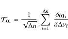
| Issue |
A&A
Volume 508, Number 2, December III 2009
|
|
|---|---|---|
| Page(s) | 877 - 887 | |
| Section | Stellar structure and evolution | |
| DOI | https://doi.org/10.1051/0004-6361/200912944 | |
| Published online | 04 November 2009 | |
A&A 508, 877-887 (2009)
On detecting the large separation in the autocorrelation of stellar oscillation times series![[*]](/icons/foot_motif.png)
B. Mosser1 - T. Appourchaux2
1 - LESIA, CNRS, Université Pierre et Marie Curie, Université Denis Diderot, Observatoire de Paris, 92195 Meudon Cedex, France
2 -
Institut d'Astrophysique Spatiale, UMR8617, Université Paris XI, Bâtiment 121, 91405 Orsay Cedex, France
Received 21 July 2009 / Accepted 7 October 2009
Abstract
Context. The observations carried out by the space missions
CoRoT and Kepler provide a large set of asteroseismic data. Their
analysis requires an efficient procedure first to determine if a star
reliably shows solar-like oscillations, second to measure the so-called
large separation, third to estimate the asteroseismic information that
can be retrieved from the Fourier spectrum.
Aims. In this paper we develop a procedure based on the
autocorrelation of the seismic Fourier spectrum that is capable of
providing measurements of the large and small frequency separations.
The performance of the autocorrelation method needs to be assessed and
quantified. We therefore searched for criteria able to predict the
output that one can expect from the analysis by autocorrelation of a
seismic time series.
Methods. First, the autocorrelation is properly scaled to take
into account the contribution of white noise. Then we use the null
hypothesis H0 test to assess the reliability of the
autocorrelation analysis. Calculations based on solar and CoRoT time
series are performed to quantify the performance as a function of the
amplitude of the autocorrelation signal.
Results. We obtain an empirical relation for the performance of
the autocorrelation method. We show that the precision of the method
increases with the observation length, and with the mean seismic
amplitude-to-background ratio of the pressure modes to the power
![]() .
We propose an automated determination of the large separation, whose reliability is quantified by the H0
test. We apply this method to analyze red giants observed by CoRoT. We
estimate the expected performance for photometric time series of the
Kepler mission. We demonstrate that the method makes it possible to
distinguish
.
We propose an automated determination of the large separation, whose reliability is quantified by the H0
test. We apply this method to analyze red giants observed by CoRoT. We
estimate the expected performance for photometric time series of the
Kepler mission. We demonstrate that the method makes it possible to
distinguish ![]() from
from ![]() modes.
modes.
Conclusions. The envelope autocorrelation function (EACF) has
proven to be very powerful for the determination of the large
separation in noisy asteroseismic data, since it enables us to quantify
the precision of the performance of different measurements: mean large
separation, variation of the large separation with frequency, small
separation and degree identification.
Key words: stars: oscillations - stars: interiors - methods: data analysis - methods: analytical
1 Introduction
Asteroseismology is known to be an efficient tool to analyze the stellar interior and to derive the physical laws that govern stellar structure and evolution. It benefits nowadays from high-performance photometric data provided by the space missions CoRoT (Baglin et al. 2006) and Kepler (Christensen-Dalsgaard et al. 2007). The amount of data is much higher than from the earlier ground-based observations, even with the recent multi-site ground-based observations (Arentoft et al. 2008), since space-borne instruments are able to simultaneously record long time series on numerous targets. The data analysis then must be efficient enough to rapidly extract seismic information from hundreds to thousands of stars.
This task is principally carried out on the frequency pattern of the eigenmodes propagating inside the stars.
For targets showing solar-like oscillations, this pattern follows the asymptotic relation of Tassoul (1980) providing eigenfrequencies nearly equally spaced by
![]() .
The eigenfrequency of radial order n and degree
.
The eigenfrequency of radial order n and degree ![]() expresses
expresses
![]() ,
,
![]() being called the large separation, D0 giving a measure of the small separation,
and
being called the large separation, D0 giving a measure of the small separation,
and
![]() a constant term.
The determination of the large separation
a constant term.
The determination of the large separation ![]() is the first step of any seismic analysis.
If the signal-to-noise ratio is high enough,
is the first step of any seismic analysis.
If the signal-to-noise ratio is high enough, ![]() can be detected by eye in the power spectrum.
In many cases, this is not possible, and the determination of
can be detected by eye in the power spectrum.
In many cases, this is not possible, and the determination of ![]() requires
sophisticated tools, as was the case for the first correct
determination of the large separation of Procyon (Mosser et al. 1998) and of the first CoRoT target observed with Doppler measurements (Mosser et al. 2005).
For observations dealing with a single target, the tools used for the determination of
requires
sophisticated tools, as was the case for the first correct
determination of the large separation of Procyon (Mosser et al. 1998) and of the first CoRoT target observed with Doppler measurements (Mosser et al. 2005).
For observations dealing with a single target, the tools used for the determination of ![]() are usually unautomated and involve parameters specific to the target.
Most often, they require the visual inspection of an image or a graph
obtained by transforming the Fourier spectrum using the asymptotic
relation cited above (échelle diagram or comb response). This step can
be automated, but with great care, since the higher order terms of
Tassoul (1980)
complicate the stacking, as does, for example, the variation of the
large separation reported in many asteroseismic targets (e.g. Mosser
et al. 2008).
are usually unautomated and involve parameters specific to the target.
Most often, they require the visual inspection of an image or a graph
obtained by transforming the Fourier spectrum using the asymptotic
relation cited above (échelle diagram or comb response). This step can
be automated, but with great care, since the higher order terms of
Tassoul (1980)
complicate the stacking, as does, for example, the variation of the
large separation reported in many asteroseismic targets (e.g. Mosser
et al. 2008).
With the advent of space photometric missions, the use of pipelines for the automatic detection of ![]() is becoming mandatory (Mathur et al. 2009)
since many targets have a low signal-to-noise ratio. A test to
determine if the large separation is reliably detected is highly
desirable, and a way to estimate the asteroseismic content of a
high-precision photometric time series will be very helpful.
is becoming mandatory (Mathur et al. 2009)
since many targets have a low signal-to-noise ratio. A test to
determine if the large separation is reliably detected is highly
desirable, and a way to estimate the asteroseismic content of a
high-precision photometric time series will be very helpful.
This paper proposes an original way to address these issues. It is based on a first report by Roxburgh & Vorontsov (2006, hereafter RV06), who analyse solar-like oscillations via the square of the autocorrelation of the time series, calculated as the Fourier spectrum of the filtered Fourier spectrum. RV06 state that the method is useful when faced with low signal-to-noise ratio data, and might be useful in obtaining information about a star even when individual frequencies cannot be extracted. Roxburgh (2009, hereafter R09) shows that it is possible, with basic and rapid computations, to attain more complex objectives, such as measurement of the variations of the large separation with frequency.
Since it provides a rapid measurement of the large separation, the autocorrelation method fits perfectly with the main asteroseismic objective of the Kepler mission, the large separation being used as an independent measurement in extracting the radius of stars hosting exoplanets, as in Stello et al. (2009). The autocorrelation achieves this goal without fitting a complex mode pattern to the stellar power spectrum. Therefore, it provides a simple tool to estimate the asteroseismic information of a Fourier spectrum or to use with Kepler, which will produce numerous time series of stellar targets.
We propose to quantify the relevance of the autocorrelation method with the null hypothesis, and to determine simple criteria to assess its efficiency and predictive power when analyzing an oscillation spectrum with a low signal-to-noise ratio. The method is also useful for extrapolating the performance obtained with a short time series to that obtained with a 4-year long time series, as will be provided by the Kepler mission. The analysis relies on photometric time series as observed by CoRoT (Baglin et al. 2006), plus simulations based on these CoRoT spectra with the addition of noise. It also includes simulations derived from a solar oscillation spectrum observed in photometry by the VIRGO/SPM instrument of the SOHO mission.
Section 2
introduces the envelope autocorrelation function (EACF) and the way we
scale it to properly account for the noise contribution. We show in
Sect. 3 how the value of
the main autocorrelation peak varies with different global parameters
of the stellar oscillation spectrum. A crucial parameter is the mean
seismic height-to-background ratio
![]() ,
representing the smoothed height of the seismic power spectral density compared to the background.
We introduce in Sect. 4 the H0
test, that allows us to examine and to quantify the performance of the
method. The value of the EACF gives a reliable criterion to estimate
the seismic output, from the determination of the mean large separation
when the signal is poor to the possibility of precise mode fitting in
other cases. Discussion of various cases is presented in Sect. 5. We propose an automated determination of the large separation; using the H0 test, we can quantify the reliability of this method. Section 6 is devoted to conclusions.
,
representing the smoothed height of the seismic power spectral density compared to the background.
We introduce in Sect. 4 the H0
test, that allows us to examine and to quantify the performance of the
method. The value of the EACF gives a reliable criterion to estimate
the seismic output, from the determination of the mean large separation
when the signal is poor to the possibility of precise mode fitting in
other cases. Discussion of various cases is presented in Sect. 5. We propose an automated determination of the large separation; using the H0 test, we can quantify the reliability of this method. Section 6 is devoted to conclusions.
2 Autocorrelation
2.1 Calculation
RV06 proposes to perform the autocorrelation of the seismic time series
as the Fourier spectrum of the filtered Fourier transform of the time
series. This directly gives the amplitude of the envelope of the
autocorrelation function, as shown in the Appendix.
Instead of the canonical form,
with
We deal with the dimensionless square module of the autocorrelation:
The choice of square module has no impact on the results presented below, but proved to be more convenient in many cases, such as the observed linear increase of
2.2 Noise scaling
In order to compare different cases, it is preferable to express the
amplitude of the autocorrelation signal in noise units. The mean noise
level in the autocorrelation can be derived from the fact that the
noise statistic is a ![]() with 2 degrees of freedom. It is expressed in the general case as:
with 2 degrees of freedom. It is expressed in the general case as:

with

With such a cosine filter and the resulting noise level, we define the EACF:

We note that
Table 1:
![]() and parameters of the p mode envelope for CoRoT targets.
and parameters of the p mode envelope for CoRoT targets.
![\begin{figure}
\par\includegraphics[width=9cm,clip]{12944_1.ps}
\end{figure}](/articles/aa/full_html/2009/47/aa12944-09/img53.png)
|
Figure 1: Contributions to the smoothed power density distribution for HD 49933. The oscillation spectrum was slightly and severely smoothed (solid thin and thick lines). The dashed line represents the contributions of granulation and photon noise. The dash-dot lines account for the Gaussian modeling of the seismic envelope and the total contribution. |
| Open with DEXTER | |
3 Analysis
We tested the variation of
![]() with various parameters, in order to determine the relevant ingredients
contributing to this signal. We based the analysis on solar data
obtained with the VIRGO/SPM instrument onboard SOHO (Frohlich
et al. 1997),
and on the CoRoT data provided on the solar-like targets HD 49933
(Appourchaux et al. 2008), HD 49385 (Deheuvels et al.,
private comm.), HD 175726 (Mosser et al. 2009), HD 181420 (Barban et al. 2009) and HD 181906 (Garcia et al. 2009). We also include the red giant HD 181907 observed by CoRoT (Carrier et al. 2009). All these targets are presented in Table 1. We also considered a set of red giants observed in the exoplanetary field of CoRoT, already analyzed by Hekker et al. (2009).
with various parameters, in order to determine the relevant ingredients
contributing to this signal. We based the analysis on solar data
obtained with the VIRGO/SPM instrument onboard SOHO (Frohlich
et al. 1997),
and on the CoRoT data provided on the solar-like targets HD 49933
(Appourchaux et al. 2008), HD 49385 (Deheuvels et al.,
private comm.), HD 175726 (Mosser et al. 2009), HD 181420 (Barban et al. 2009) and HD 181906 (Garcia et al. 2009). We also include the red giant HD 181907 observed by CoRoT (Carrier et al. 2009). All these targets are presented in Table 1. We also considered a set of red giants observed in the exoplanetary field of CoRoT, already analyzed by Hekker et al. (2009).
3.1 Seismic amplitude-to-background ratio
The strength of the autocorrelation of the time series depends on the
ratio of the mean seismic amplitude compared to all other signal and
noise. We can derive this signal-to-noise ratio in the time series from
the ratio estimated in the oscillation spectrum. This ratio in the
Fourier spectrum does not depend on the frequency resolution when the
modes are resolved, i.e. the observation time is longer than the mode
lifetime. In order to remove the influence of unknown parameters, such
as the star inclination or the mode lifetime, we have to consider the
ratio
![]() of the mode height to the background power density, at the
maximum-oscillation frequency, in a smoothed power density spectrum
(Fig. 1).
of the mode height to the background power density, at the
maximum-oscillation frequency, in a smoothed power density spectrum
(Fig. 1).
In order to estimate the background power, we have modeled the Fourier spectra with three components as in Michel et al. (2008): a low-frequency Lorentzian-like profile, a Gaussian mode envelope and a high-frequency noise. Figure 1
shows this modeling for HD 49933.
The smoothed power density depends on the filter width. In order to
avoid Gibbs phenomenon-like structures, a Gaussian filter has to be
preferred to a boxcar average. The width has to be proportional to the
large separation: a value of
![]() provides the optimum smoothing and limits the influence of the varying
background level. Since, at this stage, the large separation is a
priori unknown, the value of the filter width can be estimated with the
help of the relation found between the large separation and the
maximum-power frequency derived from the solar-like CoRoT targets:
provides the optimum smoothing and limits the influence of the varying
background level. Since, at this stage, the large separation is a
priori unknown, the value of the filter width can be estimated with the
help of the relation found between the large separation and the
maximum-power frequency derived from the solar-like CoRoT targets:
Table 1 gives
3.2 EACF as a function of time, filter width and signal-to-noise ratio
The scaling (Eq. (6)) permitted us to perform different treatments in order to analyze how the EACF varies with the observing time t, the filter width
![]() ,
the full-width at half-maximum of the mode envelope
,
the full-width at half-maximum of the mode envelope
![]() and
and
![]() .
With a linear dependence of t and the introduction of the reduced width
.
With a linear dependence of t and the introduction of the reduced width
![]() ,
we found:
,
we found:
The amplitude
Figure 2 shows
the global fit, valid for photometric data of solar-like stars obtained
with CoRoT or with VIRGO/SPM onboard SOHO. All values are fit within ![]() %, when
%, when
![]() ,
except the amplitudes for HD175726, which is the target with the lowest
,
except the amplitudes for HD175726, which is the target with the lowest
![]() ;
however, the maximum amplitude for this star agrees with the others.
;
however, the maximum amplitude for this star agrees with the others.
![\begin{figure}
\par\includegraphics[width=9cm,clip]{12944_2.ps}
\end{figure}](/articles/aa/full_html/2009/47/aa12944-09/img62.png)
|
Figure 2:
Variation of the reduced amplitude
|
| Open with DEXTER | |
We have verified that the exponent of the
![]() dependence that minimizes the dispersion of the different curves in Fig. 2 is
dependence that minimizes the dispersion of the different curves in Fig. 2 is
![]() .
A theoretical analysis should be performed to assess this result. Such
a work requires one to take into account the link between
.
A theoretical analysis should be performed to assess this result. Such
a work requires one to take into account the link between
![]() and the star inclination, the mode lifetime and the stellar noise.
and the star inclination, the mode lifetime and the stellar noise.
3.3 Maximum autocorrelation signal
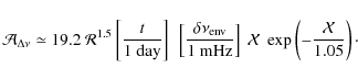
From Eq. (8), we can derive the maximum autocorrelation signal, obtained for
![]() .
It varies as:
.
It varies as:
![\begin{displaymath}
\mathcal{A}_{{\rm max}}\simeq 7.0 \ \alpha \ \mathcal{R}^{1....
...\left[{ \delta\nu_{{\rm env}}\over 1~ {\rm mHz}}\right] \cdot
\end{displaymath}](/articles/aa/full_html/2009/47/aa12944-09/img64.png)
The parameter
Figure 2 helps to identify
![]() .
For all solar-like single stars but HD 181906, the agreement with Eq. (9) is better than
.
For all solar-like single stars but HD 181906, the agreement with Eq. (9) is better than ![]() 15%.
The fact that HD 181906 shows the lowest maximum among solar-like stars is certainly due to its binarity (Bruntt 2009):
15%.
The fact that HD 181906 shows the lowest maximum among solar-like stars is certainly due to its binarity (Bruntt 2009):
![]() and
and
![]() are corrupted by the unknown contribution of the companion. The observed value of
are corrupted by the unknown contribution of the companion. The observed value of
![]() for the red giant HD 181907, not shown, is 2 times lower than
expected. This is clearly related to the narrow envelope of its
oscillation spectrum, expressed by
for the red giant HD 181907, not shown, is 2 times lower than
expected. This is clearly related to the narrow envelope of its
oscillation spectrum, expressed by
![]() compared to a mean value of 10 for solar-like stars (Table 1). The number of observed p modes is then twice as small and the EACF is reduced.
compared to a mean value of 10 for solar-like stars (Table 1). The number of observed p modes is then twice as small and the EACF is reduced.
4 Performance
The scaling of
![]() with Eq. (6) allows us to test the reliability of the detection of the large separation with the H0
test, and then to estimate the scientific output of the EACF. The null
hypothesis, term first coined by the geneticist and statistician Ronald
Fisher in Fisher (1935), consists here of assuming that the correlation is generated by pure white noise. If the EACF is high enough, the H0 hypothesis is rejected, implying that a signal might have been detected (Appourchaux 2004).
with Eq. (6) allows us to test the reliability of the detection of the large separation with the H0
test, and then to estimate the scientific output of the EACF. The null
hypothesis, term first coined by the geneticist and statistician Ronald
Fisher in Fisher (1935), consists here of assuming that the correlation is generated by pure white noise. If the EACF is high enough, the H0 hypothesis is rejected, implying that a signal might have been detected (Appourchaux 2004).
4.1 H0 test
Assessing the reliability of the measurement of the large separation as
proposed by RV06 implies applying a statistical test as the null
hypothesis H0. A priori information on the large separation may come from scaling laws (Christensen-Dalsgaard & Frandsen 1983),
or may be derived from the location of the maximum signal, or from the
initial guess of the stellar fundamental parameters. The large
separation is then searched for over a range
![]() .
The number
.
The number
![]() of independent bins over the range
of independent bins over the range
![]() depends on the width of the cosine filter. It is proportional but not equal to the number of points
depends on the width of the cosine filter. It is proportional but not equal to the number of points
![]() selected by the filter in the Fourier spectrum. It can be determined from the full width at half-maximum
selected by the filter in the Fourier spectrum. It can be determined from the full width at half-maximum
![]() of the autocorrelation peaks. Then,
of the autocorrelation peaks. Then,
![]() is:
is:

Therefore the rejection of the H0 hypothesis at probability level
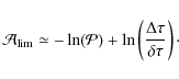
This equation is only valid if

with
As shown above, the width of the best filter giving the maximum
autocorrelation signal is proportional to the width of the seismic mode
envelope,
![]() ,
and the mode envelope also varies almost linearly with the the large separation,
,
and the mode envelope also varies almost linearly with the the large separation,
![]() .
This gives
.
This gives
![]() .
As a consequence, independent of the large separation, the number of
independent bins in the autocorrelation can be estimated by:
.
As a consequence, independent of the large separation, the number of
independent bins in the autocorrelation can be estimated by:

Setting the mean optimum value of
![\begin{figure}
\par\includegraphics[width=9cm,clip]{12944_3.ps}
\end{figure}](/articles/aa/full_html/2009/47/aa12944-09/img81.png)
|
Figure 3:
Precision of the function
|
| Open with DEXTER | |
![\begin{figure}
\par\includegraphics[width=9cm,clip]{12944_4.ps}
\end{figure}](/articles/aa/full_html/2009/47/aa12944-09/img82.png)
|
Figure 4: Same as Fig. 3, but for HD 181420. |
| Open with DEXTER | |
4.2 Determination of the mean large separation

The determination of the mean value of the large separation requires
![]() to be greater than a threshold value of about 8 for a detection at the 1% rejection level. From Eq. (A.8), we then get an estimate of the relative precision of the mean large separation
to be greater than a threshold value of about 8 for a detection at the 1% rejection level. From Eq. (A.8), we then get an estimate of the relative precision of the mean large separation
![]() ,
integrated over a large frequency centered on the maximum-oscillation frequency:
,
integrated over a large frequency centered on the maximum-oscillation frequency:
At the detection limit
4.3 Variation of the large separation with frequency
With smaller values of
![]() ,
it is possible to address the variation of the large separation with frequency as explained in R09. Investigating in detail
,
it is possible to address the variation of the large separation with frequency as explained in R09. Investigating in detail
![]() requires a filter
requires a filter
![]() much narrower than
much narrower than
![]() ,
so that we can derive
,
so that we can derive
![]() from Eq. (8). In this case, the best relative precision at the maximum oscillation frequency can be derived from Eq. (A.8):
from Eq. (8). In this case, the best relative precision at the maximum oscillation frequency can be derived from Eq. (A.8):
The scaling to the large separation insures a uniform precision throughout the HR diagram. With
![\begin{figure}
\par\includegraphics[width=9cm,clip]{12944_5.ps}
\end{figure}](/articles/aa/full_html/2009/47/aa12944-09/img89.png)
|
Figure 5:
Function
|
| Open with DEXTER | |
![\begin{figure}
\par\includegraphics[width=9cm,clip]{12944_6.ps}
\end{figure}](/articles/aa/full_html/2009/47/aa12944-09/img90.png)
|
Figure 6:
Function
|
| Open with DEXTER | |
4.4 Disentangling the degree
Examining the half-separations
![]() and
and
![]() ,
as proposed by R09, requires
,
as proposed by R09, requires
![]() narrower than
narrower than ![]() .
We have found that
.
We have found that
![]() provides the best compromise: it is narrow enough to select only 1 pair
of modes with degree 0 and 1, and large enough to give an accurate
signal-to-ratio.
Setting
provides the best compromise: it is narrow enough to select only 1 pair
of modes with degree 0 and 1, and large enough to give an accurate
signal-to-ratio.
Setting
![]() ,
a 1% precision on the determination of
,
a 1% precision on the determination of ![]() requires
requires
![]() ,
which is achieved only for HD 49933 and HD 49385.
,
which is achieved only for HD 49933 and HD 49385.
As reported by R09, the different half-large separations are clearly distinguished.
However, values are correlated within the filter, and mixed with other separations including ![]() modes. Therefore, we do not consider that the autocorrelation is able
to provide a precise measurement of the half-separations. For instance,
we cannot reproduce the Solar values (Fig. 5).
However, we clearly show that the local minima match the
eigenfrequencies with high precision. We observed, in the unambiguous
cases provided by the Sun, HD 49385 (Fig. 6) and models, that the local minima associated with
modes. Therefore, we do not consider that the autocorrelation is able
to provide a precise measurement of the half-separations. For instance,
we cannot reproduce the Solar values (Fig. 5).
However, we clearly show that the local minima match the
eigenfrequencies with high precision. We observed, in the unambiguous
cases provided by the Sun, HD 49385 (Fig. 6) and models, that the local minima associated with ![]() are lower than the ones with
are lower than the ones with ![]() .
This is due to the fact that, under the assumption of a Tassoul-like spectrum, a narrow filter centered on the
.
This is due to the fact that, under the assumption of a Tassoul-like spectrum, a narrow filter centered on the ![]() mode tests the separations
mode tests the separations
![]() and
and
![]() ,
whereas a narrow filter centered on the
,
whereas a narrow filter centered on the ![]() mode tests the separations
mode tests the separations
![]() and
and
![]() .
In the asymptotic formalism,
.
In the asymptotic formalism,
![]() is significantly smaller than
is significantly smaller than
![]() (by an amount of 4 D0).
(by an amount of 4 D0).
When the filter is not centered on an eigenmode, it mainly tests the separation
![]() or
or
![]() .
Therefore, we show that a narrow frequency windowed autocorrelation allows us to distinguish
.
Therefore, we show that a narrow frequency windowed autocorrelation allows us to distinguish ![]() from
from ![]() ,
which is a crucial issue since many observations have shown how difficult it can be to distinguish them (Barban et al. 2009; Garcia et al. 2009). The test applied to the first initial run on HD 49933 (Fig. 7) shows that the former mode identification of Appourchaux et al. (2008) cannot be confirmed, as also shown by Benomar et al. (private comm.) who analyze a second longer run.
,
which is a crucial issue since many observations have shown how difficult it can be to distinguish them (Barban et al. 2009; Garcia et al. 2009). The test applied to the first initial run on HD 49933 (Fig. 7) shows that the former mode identification of Appourchaux et al. (2008) cannot be confirmed, as also shown by Benomar et al. (private comm.) who analyze a second longer run.
![\begin{figure}
\par\includegraphics[width=9cm,clip]{12944_7.ps}\vspace*{2.5mm}
\includegraphics[width=9cm,clip]{12944_8.ps}
\end{figure}](/articles/aa/full_html/2009/47/aa12944-09/img98.png)
|
Figure 7:
Function
|
| Open with DEXTER | |
A clear identification requires a signal-to-noise ratio high enough. Again, Eq. (15) allows us to estimate the autocorrelation amplitude required. In order to distinguish the small separation D0, and considering as a rough estimate that in the mean case D0 represents about 2% of the large separation, a reliable determination based on a narrow filter
![]() requires a maximum amplitude greater than about 200.
requires a maximum amplitude greater than about 200.
Table 2: Degree identification.
![\begin{figure}
\par\includegraphics[width=9cm,clip]{12944_9.ps}
\vspace*{2mm}\end{figure}](/articles/aa/full_html/2009/47/aa12944-09/img102.png)
|
Figure 8: Same as Fig. 7, but for HD 181420. |
| Open with DEXTER | |
![\begin{figure}
\par\includegraphics[width=9cm,clip]{12944_10.ps}
\end{figure}](/articles/aa/full_html/2009/47/aa12944-09/img103.png)
|
Figure 9: Same as Fig. 7, but for HD 181906 and with a broader filter. The large uncertainty indicated by the broad grey region shows that the identification for that star is not reliable. |
| Open with DEXTER | |
Table 2 summarizes the mean value of the difference
![]() between the local minima compared to the 1-
between the local minima compared to the 1-![]() uncertainty
uncertainty
![]() of the narrow frequency windowed autocorrelation function (Eq. (15)):
of the narrow frequency windowed autocorrelation function (Eq. (15)):
with
This criterion helps to explain why the ridges can be unambiguously
identified in HD 49385 (Deheuvels et al., private comm.) and why
scenario 1 for HD 181420 must be preferred (Barban et al. 2009): Figs. 7 and 8 show that the mean difference between the local minimal corresponding to ![]() or 1 is greater than the error bar of
or 1 is greater than the error bar of
![]() .
On the other hand, no answer can be given for HD 181906 (Garcia et al. 2009): the low value of
.
On the other hand, no answer can be given for HD 181906 (Garcia et al. 2009): the low value of
![]() hampers the calculation of
hampers the calculation of
![]() with a narrow filter (Fig. 9).
The limited
with a narrow filter (Fig. 9).
The limited
![]() for the initial run on HD 49933 and the low value
for the initial run on HD 49933 and the low value
![]() help to explain the difficulties encountered with the mode identification given in Appourchaux et al. (2008).
help to explain the difficulties encountered with the mode identification given in Appourchaux et al. (2008).
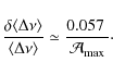
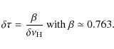
4.5 Ultimate precision on

Obtaining the best time resolution in the EACF, namely the time resolution 
According to this, high precision is easier to reach for high
4.6 Small separation
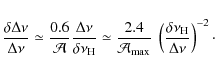
Roxburgh & Vorontsov (2006) proposed to make use of the autocorrelation function to obtain an independent estimate of the small separation. This method is based on the comparison of the peak amplitude of even or odd orders in the autocorrelation function. WithTable 3: Threshold levels.
4.7 Threshold levels
Table 3 summarizes the
threshold levels for the determination of the seismic parameters with
the EACF. At low signal-to-noise ratios, namely an
![]() value lower than 8, the method cannot operate, according to the H0 test. Then, the domain where the autocorrelation is highly performing is for
value lower than 8, the method cannot operate, according to the H0 test. Then, the domain where the autocorrelation is highly performing is for
![]() ranging from 8 (detection limit) to
ranging from 8 (detection limit) to
![]() ,
when precise mode fitting becomes possible (HD 181906, Garcia et al. 2009). With
,
when precise mode fitting becomes possible (HD 181906, Garcia et al. 2009). With
![]() value up to 200, the EACF may be useful for identifying the degree of
the modes, under the condition that the oscillation spectrum is close
to a Tassoul-like pattern. Larger
value up to 200, the EACF may be useful for identifying the degree of
the modes, under the condition that the oscillation spectrum is close
to a Tassoul-like pattern. Larger
![]() values allow a more detailed analysis with classical methods such as mode fitting (Appourchaux et al. 2006).
values allow a more detailed analysis with classical methods such as mode fitting (Appourchaux et al. 2006).
![\begin{figure}
\par\includegraphics[width=9cm,clip]{12944_11.ps}\vspace*{2mm}
\end{figure}](/articles/aa/full_html/2009/47/aa12944-09/img121.png)
|
Figure 10:
Automatic search for the signature of a large separation for
HD 49933. The grey line indicates the location of the maximum
peak, corresponding to the mean large separation of the star. The
horizontal segments indicate the ranges corresponding to the 13 initial
guess values
|
| Open with DEXTER | |
5 Discussion
5.1 Automated determination of the large separation
Autocorrelation may provide an effective automatic determination of the large separation when nothing is known about the star, as can be the case for a Kepler target. As shown previously, testing the autocorrelation aroundThe automatic test consists of analyzing the autocorrelation of the time series for a set of time shifts
![]() in geometrical progression. We performed the automatic autocorrelation test with 13 values of
in geometrical progression. We performed the automatic autocorrelation test with 13 values of
![]() ,
varying from 3 to 192
,
varying from 3 to 192 ![]() Hz with a geometric ratio G equal to
Hz with a geometric ratio G equal to ![]() ;
;
![]() can be considered as an initial guess of the large separation. For each initial value
can be considered as an initial guess of the large separation. For each initial value
![]() ,
we explored the range
,
we explored the range
![]() of the autocorrelation for
3 frequency ranges of the Fourier spectrum centered respectively around
of the autocorrelation for
3 frequency ranges of the Fourier spectrum centered respectively around
![]() and
and
![]() .
We finally derived the large separation from the maximum amplitude
.
We finally derived the large separation from the maximum amplitude
![]() calculated for each
calculated for each
![]() initial guess. Comparison of the different
initial guess. Comparison of the different
![]() is made possible by the scaling provided by Eq. (6). Figure 10 shows the result for HD 49933.
is made possible by the scaling provided by Eq. (6). Figure 10 shows the result for HD 49933.
![\begin{figure}
\par\includegraphics[width=9cm,clip]{12944_12.ps}
\end{figure}](/articles/aa/full_html/2009/47/aa12944-09/img129.png)
|
Figure 11: Same as Fig. 10, but for HD 175726. The dashed line indicates the 10% rejection limit. |
| Open with DEXTER | |
We also tested the automatic test with the stars with the lowest
![]() ,
namely HD175726 and HD 181907.
For HD 175726, the single value exceeding the 10% rejection level occurs at 97
,
namely HD175726 and HD 181907.
For HD 175726, the single value exceeding the 10% rejection level occurs at 97 ![]() Hz (Fig. 11). This value of
Hz (Fig. 11). This value of ![]() agrees with the solution proposed by Mosser et al. (2009). This
detection is poor since a significance level of 10% means that the
posterior probability of the null hypothesis is at least 38% according
to Appourchaux et al. (2009).
However, the automatic detection can be refined with a dedicated search
with a more precise grid of analysis. In the case of HD 175726, the
clear identification of an excess power centered at 2 mHz first
allows us to better estimate the parameters for searching
agrees with the solution proposed by Mosser et al. (2009). This
detection is poor since a significance level of 10% means that the
posterior probability of the null hypothesis is at least 38% according
to Appourchaux et al. (2009).
However, the automatic detection can be refined with a dedicated search
with a more precise grid of analysis. In the case of HD 175726, the
clear identification of an excess power centered at 2 mHz first
allows us to better estimate the parameters for searching ![]() and, second, gives a further indication that the measurement is reliable thanks to Eq. (7).
and, second, gives a further indication that the measurement is reliable thanks to Eq. (7).
The amplitude
![]() of the automatic test is found to be close to the maximum amplitude
of the automatic test is found to be close to the maximum amplitude
![]() .
Only limited fine tuning around the automatically fixed parameters is
needed to optimize the result. Mosser et al. (2009) have mentioned
the difficulty of determining the large separation with other methods.
The autocorrelation method proves to be powerful for a rapid estimate
of the large separation; rapidity means here a few seconds of CPU time
for the Fourier spectrum of the CoRoT time series, followed by a few
seconds of CPU time for the automatic search with the autocorrelation,
with a common laptop.
.
Only limited fine tuning around the automatically fixed parameters is
needed to optimize the result. Mosser et al. (2009) have mentioned
the difficulty of determining the large separation with other methods.
The autocorrelation method proves to be powerful for a rapid estimate
of the large separation; rapidity means here a few seconds of CPU time
for the Fourier spectrum of the CoRoT time series, followed by a few
seconds of CPU time for the automatic search with the autocorrelation,
with a common laptop.
We verified that the method is effective for all other solar-like targets: it gives one single answer for ![]() ,
and does not deliver any false positives. The case of red giants requires a dedicated analysis.
,
and does not deliver any false positives. The case of red giants requires a dedicated analysis.
5.2 Red giants
We tested the method on the CoRoT red giant target HD 181907 (Carrier et al. 2009).
With a large
![]() for this target (about 2) and a large
for this target (about 2) and a large
![]() autocorrelation signal, the large separation is easily found around 3.5
autocorrelation signal, the large separation is easily found around 3.5 ![]() Hz, but the detection is polluted by many values clearly above the 1% rejection limit (Fig. 12).
All these spurious detections are caused by artefacts: detection of the
double of the large separation; detection of the diurnal frequency and
its harmonics; detection of the CoRoT orbital frequency and half its
value. We checked that the detections at high harmonics of the diurnal
frequency are due to residuals of the window function (Mosser
et al. 2009); they are introduced by the link between
Hz, but the detection is polluted by many values clearly above the 1% rejection limit (Fig. 12).
All these spurious detections are caused by artefacts: detection of the
double of the large separation; detection of the diurnal frequency and
its harmonics; detection of the CoRoT orbital frequency and half its
value. We checked that the detections at high harmonics of the diurnal
frequency are due to residuals of the window function (Mosser
et al. 2009); they are introduced by the link between
![]() and
and ![]() indicated by Eq. (7).
indicated by Eq. (7).
For HD 181907, Eq. (9) is valid within 30%. As discussed in Sect. 3, the discrepancy compared to solar-like stars is due to the fact that the mode envelope of red giants is narrower than in solar-like stars.
The automated determination of the large frequency has been
also tested on a set of 392 giants observed in the CoRoT field
dedicated to exoplanetary science and analyzed by Hekker et al. (2009).
The method proves to be efficient and rapid. It provides a clear
advantage since it gives a quantified reliability thanks to the use of
the H0 test. We present in Fig. 13 the results obtained for these giants. The maximum oscillation frequency was calculated by Hekker et al. (2009).
The amplitude of the autocorrelation signal allows us to clearly
discriminate artefacts from reliable detection (60% of the targets).
The relative precision in the mean large separation is much better than
1%, according to Eq. (14).
After correction of the stars for which the double of the large
separation is preferably automatically detected, we define from the fit
of the relation between the large separation and the location of the
maximum signal a power law varying as:
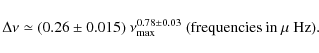
This law for giants is in agreement with Eq. (7) based on dwarfs and with Hekker et al. (2009).
Table 4: Kepler performance.
![\begin{figure}
\par\includegraphics[width=9cm,clip]{12944_13.eps}
\vspace*{3mm}
\end{figure}](/articles/aa/full_html/2009/47/aa12944-09/img132.png)
|
Figure 12:
Same as Fig. 11,
but for the red giant HD 181907. The horizontal dashed lines
indicate the 10% and 1% rejection limits. The vertical grey lines
indicate the signature at |
| Open with DEXTER | |
5.3 Kepler data
![\begin{figure}
\par\includegraphics[width=9cm,clip]{12944_14.eps}
\end{figure}](/articles/aa/full_html/2009/47/aa12944-09/img133.png)
|
Figure 13:
Large separation, automatically measured for a set of 392 red giants analyzed in Hekker et al. (2009), as a function of the maximum oscillation frequency
|
| Open with DEXTER | |
The Kepler mission compared to CoRoT will provide different photometric
performance, on dimmer targets but in some cases with longer
observation duration (Christensen-Dalsgaard et al. 2007). According to Kepler performance (Kjeldsen et al. 2008), the noise level is about 0.92, 10.2 and 144 ppm![]() Hz-1 for targets of V magnitude respectively equal to 9, 11.5 and 14.
Hz-1 for targets of V magnitude respectively equal to 9, 11.5 and 14.
We can extrapolate the performance obtained with Kepler on targets
similar to the ones observed by CoRoT, but of magnitude 9 to 14,
after a 4-year long observation. Table 4 gives the amplitude
![]() for targets observed during typical 90-day or 4-year long runs.
According to the expected performance in 90-day runs, the brightest
F-type or the class IV targets will have a signal-to-noise ratio high
enough to derive information on the large separation. In a 4-year run,
the brightest G dwarfs will deliver a clean seismic signature. On the
other hand, faint F targets will have fully exploitable Fourier spectra
that will require a precise mode fitting for the most complete seismic
analysis. The performance for giants appears to be almost independent
of the magnitude, since the contribution of photon noise is negligible
at low frequency.
for targets observed during typical 90-day or 4-year long runs.
According to the expected performance in 90-day runs, the brightest
F-type or the class IV targets will have a signal-to-noise ratio high
enough to derive information on the large separation. In a 4-year run,
the brightest G dwarfs will deliver a clean seismic signature. On the
other hand, faint F targets will have fully exploitable Fourier spectra
that will require a precise mode fitting for the most complete seismic
analysis. The performance for giants appears to be almost independent
of the magnitude, since the contribution of photon noise is negligible
at low frequency.
We can compare this approach to the hare-and-hounds exercises performed by Chaplin et al. (2008). The asteroseismic goal of Kepler is principally to derive information on stars hosting a planet, by the determination of the large separation. Compared to global fitting, the autocorrelation function gives a more rapid and direct answer.
The autocorrelation benefits from the rapid cadence (32 s) provided by CoRoT in the seismology field. Kepler will provide 2 cadences, at 1 or 30 min. This yields a lower resolution in time, hence a lower precision on the expected results.
6 Conclusion
Roxburgh & Vorontsov (2006)
have proposed a method for estimating large and small separations from
the analysis of the autocorrelation function. Roxburgh (2009)
has extended the method to determine the variation of the large
separation. In this paper, we have developed and quantified the method,
relating the amplitude of the correlation peak at time shift
![]() to various parameters.
to various parameters.
We have scaled the autocorrelation to the white noise contribution, so
that we were able to relate the autocorrelation signal to the mean
seismic height-to-background ratio
![]() that measures the relative power density of the signal compared to
noise and to background signals. This empirical relation is precise to
about 15% for solar-like stars.
that measures the relative power density of the signal compared to
noise and to background signals. This empirical relation is precise to
about 15% for solar-like stars.
![]() aggregates the influence of unknown parameters such as the mode
lifetimes, the star inclination (that governs the modes visibility) or
the rotational splitting. On the other hand, all these unknown
parameters complicate and slow down the fitting of individual
eigenfrequencies. Therefore, the EACF shows here a possible advantage
in terms of speed.
aggregates the influence of unknown parameters such as the mode
lifetimes, the star inclination (that governs the modes visibility) or
the rotational splitting. On the other hand, all these unknown
parameters complicate and slow down the fitting of individual
eigenfrequencies. Therefore, the EACF shows here a possible advantage
in terms of speed.
The EACF gives a direct measurement of the mean large
separation. Compared to other methods, the estimate is accurate and
simple, with an intrinsic threshold value, with error bars, and without
any modeling of the other components of the Fourier spectrum
(granulation or activity). Furthermore, when the signal-to-noise ratio
is high enough, the EACF allows the measurement of the variation of the
large separation with frequency, without any mode fitting. This is a
key point for stellar radius measurement.
Previous works have shown the difficulty to disentangle ![]() from
from ![]() modes in oscillation spectra of F stars observed in photometry. We have
verified that, for high signal-to-noise ratio Fourier spectra, the
autocorrelation analysis can provide an unambiguous identification of
the mode degree for a solar-like oscillation spectrum.
modes in oscillation spectra of F stars observed in photometry. We have
verified that, for high signal-to-noise ratio Fourier spectra, the
autocorrelation analysis can provide an unambiguous identification of
the mode degree for a solar-like oscillation spectrum.
We have defined a method for the automatic determination of the large separation, which is efficient at low signal-to-noise ratio, even if no information is known for the star. We have determined that the width of the cosine filter used in the method that optimizes the EACF is very close to full-width at half-maximum of the mode envelope (ratio about 1.05). We have also checked that the performance of the method increases linearly with the duration of the time series. With very limited CPU time (a few seconds), this method delivers the mean large separation of a target. It requires no information on the star; it just relies on the assumption that the location of the excess power and its width are related to the large separation by a scaling law, what is verified for red giants and solar-like stars. Finally, we were able to investigate in a simple manner the capability of Kepler.
We are confident that the autocorrelation method will be of great help in analyzing high duty cycle time series as a complement to the Fourier analysis. As noticed by Fossat et al. (1999), the autocorrelation signal gives a clear signature since the autocorrelation delay, namely four times the stellar acoustic radius (about 4 to 8 h for an F dwarf), is much shorter than the mode lifetime (a few days). This allows each wavepacket to properly correlate with itself after a double travel along the stellar diameter, so that the autocorrelation integrates phased responses over the total duration time. In the Fourier spectrum, on the contrary, interference between the short-lived wavepackets observed in the time series produce a complicated pattern. But Fourier analysis still remains required for the precise determination of the eigenfrequencies derived from an accurate mode fitting.
Appendix A: Performance of the autocorrelation
A.1 Square module of the autocorrelation
The EACF presented in Sect. 2
is defined to directly give the envelope of the autocorrelation. Since
negative frequencies are omitted, the EACF is related to the canonical
autocorrelation
![]() ,
that includes positive and negative frequencies of the Fourier spectrum, by:
,
that includes positive and negative frequencies of the Fourier spectrum, by:
where
![\begin{figure}
\par\includegraphics[width=9cm,clip]{12944_15.ps}
\end{figure}](/articles/aa/full_html/2009/47/aa12944-09/img140.png)
|
Figure A.1:
Comparison of
|
| Open with DEXTER | |
![\begin{figure}
\par\includegraphics[width=9cm,clip]{12944_16.ps}
\end{figure}](/articles/aa/full_html/2009/47/aa12944-09/img142.png)
|
Figure A.2:
Autocorrelation peak
|
| Open with DEXTER | |
A.2 Autocorrelation peak
The shape of the autocorrelation peaks is given by the Fourier
transform of the Hanning filter, which can be expressed as the sum of 3
components (Max & Lacoume 1996):
with
The flanks of the peak are not well fitted, which is unimportant compared to the fact that the fit above half-maximum performs well.
Precise determination of the large separation requires precise location
of the peak maximum. In order to estimate the performance, we describe
a peak as:
|
(A.4) |
This fit shows variation:
|
(A.5) |
We can compare the variation of the signal peaking at amplitude
|
(A.6) |
The precise identification of the signal maximum requires
It is possible to interpret this condition as follows.
A.3 Precision on the mean large separation
If the amplitude is not large enough, then Eq. (A.7) defines a resolution ![]() ,
hence a limited precision on the large separation:
,
hence a limited precision on the large separation:
We can set, as a limit to detection, b =5 and
A.4 Full resolution for the measurement of
In order to recover the full time resolution
![]() ,
the amplitude must satisfy
,
the amplitude must satisfy
![]() ,
with the definition:
,
with the definition:
With b=5:

Acknowledgements
This work was supported by the Centre National d'Etudes Spatiales (CNES). It is based on observations with CoRoT. Solar data were obtained from SOHO, a mission of international collaboration between ESA and NASA.
The work has benefitted from simulating discussions among asteroseismologists working on the excellent CoRoT data. B.M. thanks Ian Roxburgh for motivating discussions, and John Leibacher for helpful comments. We thank Saskia Hekker and Caroline Barban for providing us with the red giant data and the values of the maximum frequency plotted in Fig. 13.
References
- Appourchaux, T. 2004, A&A, 428, 1039 [NASA ADS] [EDP Sciences] [CrossRef]
- Appourchaux, T., Berthomieu, G., Michel, E., et al. 2006, ESA SP, 1306, 377 [NASA ADS]
- Appourchaux, T., Michel, E., Auvergne, M., et al. 2008, A&A, 488, 705 [NASA ADS] [EDP Sciences] [CrossRef]
- Appourchaux, T., Samadi, R., & Dupret, M.-A. 2009, A&A, 506, 1 [EDP Sciences] [CrossRef]
- Arentoft, T., Kjeldsen, H., Bedding, T. R., et al. 2008, ApJ, 687, 1180 [NASA ADS] [CrossRef]
- Auvergne, M., Bodin, P., Boisnard, L., et al. 2009, A&A, 506, 411 [EDP Sciences] [CrossRef]
- Baglin, A., Auvergne, M., Barge, P., et al. 2006, ESA SP, 1306, 33 [NASA ADS]
- Barban, C., Deheuvels, S., Baudin, F., et al. 2009, A&A, 506, 51 [EDP Sciences] [CrossRef]
- Bruntt, H. 2009, A&A, 506, 235 [EDP Sciences] [CrossRef]
- Carrier, F., De Ridder, J., Baudin, F., et al. 2009, A&A, accepted
- Chaplin, W. J., Appourchaux, T., Arentoft, T., et al. 2008, Astron. Nachr., 329, 549 [NASA ADS] [CrossRef]
- Christensen-Dalsgaard, J., & Frandsen, S. 1983, Sol. Phys., 82, 469 [NASA ADS] [CrossRef]
- Christensen-Dalsgaard, J., Arentoft, T., Brown, T. M., et al. 2007, Commun. Asteroseismol., 150, 350 [NASA ADS] [CrossRef]
- Fischer, R. A. 1935, The Design of Experiments (Edinburgh: Oliver and Boyd), 18
- Fossat, E., Kholikov, Sh., Gelly, B., et al. 1999, A&A, 343, 608 [NASA ADS]
- Frohlich, C., Andersen, B. N., Appourchaux, T., et al. 1997, Sol. Phys., 170, 1 [NASA ADS] [CrossRef]
- Garcia, R. A., Régulo, C., Samadi, R., et al. 2009, A&A, 506, 41 [EDP Sciences] [CrossRef]
- Kjeldsen, H., Bedding, T. R., Viskum, M., & Frandsen, S. 1995, AJ, 109, 1313 [NASA ADS] [CrossRef]
- Kjeldsen, H., et al. 2008, KASC target selection procedure: Instructions, http://astro.phys.au.dk/KASC/DASC_KASOC_0008_5.pdf
- Hekker S., Kallinger, T., Baudin, F., et al. 2009, A&A, 506, 465 [EDP Sciences] [CrossRef]
- Mathur, S., Garcia, R. A., Regulo, C., et al. 2009, A&A, submitted [arXiv:0907.1139]
- Max, J., & Lacoume, J. L. 1996, Méthodes et techniques du traitement du signal (Dunod)
- Michel, É., Baglin, A., Auvergne, M., et al. 2008, Science, 322, 558 [NASA ADS] [CrossRef]
- Mosser, B., Maillard, J. P., Mekarnia, D., & Gay, J. 1998, A&A, 340, 457 [NASA ADS]
- Mosser, B., Bouchy, F., Catala, C., et al. 2005, A&A, 431, L13 [NASA ADS] [EDP Sciences] [CrossRef]
- Mosser, B., Deheuvels, S., Michel, E., et al. 2008, A&A, 488, 635 [NASA ADS] [EDP Sciences] [CrossRef]
- Mosser, B., Roxburgh, I., Michel, E., et al. 2009, A&A, 506, 33 [EDP Sciences] [CrossRef]
- Roxburgh, I. 2009, A&A, 506, 435 [EDP Sciences] [CrossRef]
- Roxburgh, I. W., & Vorontsov, S. V. 2006, MNRAS, 369, 1491 [NASA ADS] [CrossRef]
- Stello, D., Chaplin, W. J., Bruntt, H., et al. 2009, ApJ, 700, 1589 [NASA ADS] [CrossRef]
- Tassoul, M. 1980, ApJS, 43, 469 [NASA ADS] [CrossRef]
Footnotes
- ... series
- The CoRoT space mission, launched on 2006 December 27, was developed and is operated by the CNES, with participation of the Science Programs of ESA, ESA's RSSD, Austria, Belgium, Brazil, Germany and Spain.
All Tables
Table 1:
![]() and parameters of the p mode envelope for CoRoT targets.
and parameters of the p mode envelope for CoRoT targets.
Table 2: Degree identification.
Table 3: Threshold levels.
Table 4: Kepler performance.
All Figures
|
|
Figure 1: Contributions to the smoothed power density distribution for HD 49933. The oscillation spectrum was slightly and severely smoothed (solid thin and thick lines). The dashed line represents the contributions of granulation and photon noise. The dash-dot lines account for the Gaussian modeling of the seismic envelope and the total contribution. |
| Open with DEXTER | |
| In the text | |
|
|
Figure 2:
Variation of the reduced amplitude
|
| Open with DEXTER | |
| In the text | |
|
|
Figure 3:
Precision of the function
|
| Open with DEXTER | |
| In the text | |
|
|
Figure 4: Same as Fig. 3, but for HD 181420. |
| Open with DEXTER | |
| In the text | |
|
|
Figure 5:
Function
|
| Open with DEXTER | |
| In the text | |
|
|
Figure 6:
Function
|
| Open with DEXTER | |
| In the text | |
|
|
Figure 7:
Function
|
| Open with DEXTER | |
| In the text | |
|
|
Figure 8: Same as Fig. 7, but for HD 181420. |
| Open with DEXTER | |
| In the text | |
|
|
Figure 9: Same as Fig. 7, but for HD 181906 and with a broader filter. The large uncertainty indicated by the broad grey region shows that the identification for that star is not reliable. |
| Open with DEXTER | |
| In the text | |
|
|
Figure 10:
Automatic search for the signature of a large separation for
HD 49933. The grey line indicates the location of the maximum
peak, corresponding to the mean large separation of the star. The
horizontal segments indicate the ranges corresponding to the 13 initial
guess values
|
| Open with DEXTER | |
| In the text | |
|
|
Figure 11: Same as Fig. 10, but for HD 175726. The dashed line indicates the 10% rejection limit. |
| Open with DEXTER | |
| In the text | |
|
|
Figure 12:
Same as Fig. 11,
but for the red giant HD 181907. The horizontal dashed lines
indicate the 10% and 1% rejection limits. The vertical grey lines
indicate the signature at |
| Open with DEXTER | |
| In the text | |
|
|
Figure 13:
Large separation, automatically measured for a set of 392 red giants analyzed in Hekker et al. (2009), as a function of the maximum oscillation frequency
|
| Open with DEXTER | |
| In the text | |
|
|
Figure A.1:
Comparison of
|
| Open with DEXTER | |
| In the text | |
|
|
Figure A.2:
Autocorrelation peak
|
| Open with DEXTER | |
| In the text | |
Copyright ESO 2009
Current usage metrics show cumulative count of Article Views (full-text article views including HTML views, PDF and ePub downloads, according to the available data) and Abstracts Views on Vision4Press platform.
Data correspond to usage on the plateform after 2015. The current usage metrics is available 48-96 hours after online publication and is updated daily on week days.
Initial download of the metrics may take a while.