| Issue |
A&A
Volume 508, Number 2, December III 2009
|
|
|---|---|---|
| Page(s) | 725 - 735 | |
| Section | Interstellar and circumstellar matter | |
| DOI | https://doi.org/10.1051/0004-6361/200912806 | |
| Published online | 27 October 2009 | |
A&A 508, 725-735 (2009)
Fragmentation of a dynamically condensing radiative layer
K. Iwasaki - T. Tsuribe
Department of Earth and Space Science, Graduate School of Science, Osaka University, Toyonaka, Osaka 560-0043, Japan
Received 1 July 2009 / Accepted 14 September 2009
Abstract
In this paper,
the stability of a dynamically condensing radiative gas layer is investigated by linear
analysis.
Our own time-dependent, self-similar solutions describing a dynamical condensing
radiative gas layer are used as an unperturbed state.
We consider perturbations that are both perpendicular and parallel
to the direction of condensation.
The transverse wave number of the perturbation is defined by k.
For k=0, it is found that the condensing gas layer is unstable. However,
the growth rate is too low to become nonlinear during dynamical condensation.
For ![]() ,
in general,
perturbation equations for constant wave number cannot be reduced to
an eigenvalue problem
due to the unsteady unperturbed state.
Therefore, direct numerical integration of the perturbation equations is performed.
For comparison, an eigenvalue problem neglecting the time evolution
of the unperturbed state
is also solved and both results agree well.
The gas layer is unstable for all wave numbers, and the growth rate depends a little
on wave number.
The behaviour of the perturbation is specified by
,
in general,
perturbation equations for constant wave number cannot be reduced to
an eigenvalue problem
due to the unsteady unperturbed state.
Therefore, direct numerical integration of the perturbation equations is performed.
For comparison, an eigenvalue problem neglecting the time evolution
of the unperturbed state
is also solved and both results agree well.
The gas layer is unstable for all wave numbers, and the growth rate depends a little
on wave number.
The behaviour of the perturbation is specified by
![]() at the centre, where
the cooling length,
at the centre, where
the cooling length,
![]() ,
represents the length that a sound wave can travel
during the cooling time. For
,
represents the length that a sound wave can travel
during the cooling time. For
![]() ,
the perturbation grows isobarically.
For
,
the perturbation grows isobarically.
For
![]() ,
the perturbation grows because each part has a different collapse time without interaction.
Since the growth rate is sufficiently high, it is not long before the perturbations become nonlinear
during the dynamical condensation. Therefore, according to the linear analysis,
the cooling layer is expected to
split into fragments with various scales.
,
the perturbation grows because each part has a different collapse time without interaction.
Since the growth rate is sufficiently high, it is not long before the perturbations become nonlinear
during the dynamical condensation. Therefore, according to the linear analysis,
the cooling layer is expected to
split into fragments with various scales.
Key words: hydrodynamics - instabilities - ISM: kinematics and dynamics - ISM: structure - ISM: clouds
1 Introduction
In the interstellar medium (ISM), it is well known that a clumpy low-temperature phase (cold neutral medium, or CNM) and a diffuse high-temperature phase (warm neutral medium, or WNM) can coexist in pressure equilibrium as a result of the balance of radiative cooling and heating due to external radiation fields and cosmic rays (Field et al. 1969; Wolfire et al. 2003,1995). These two phases are thermally stable. On the other hand, gas is thermally unstable in the temperature range between two stable phases, that is, in the rangeThe basic properties of TI was investigated by Field (1965), who performed linear analysis of an uniform gas in thermally equilibrium. He derived a criterion for TI. Focusing on one fluid element, Balbus (1986) generalized the Field criterion when the cooling rate is not equal to the heating rate. The effect of magnetic field on TI has been investigated by Field (1965) and Hennebelle & Passot (2006), and other authors.
Recently, many authors have used multi-dimensional numerical simulations to study the turbulent CNM formation driven by TI. Koyama & Inutsuka (2002) suggest that the turbulent CNM formation is induced by TI in a shock-compressed region. Analogous processes have been studied by many authors for a colliding flow of the WNM (Audit & Hennebelle 2005; Vazquez-Semadeni et al. 2007; Heitsch et al. 2006; Hennebelle & Audit 2007), and using two-fluid MHD simulation (Inoue & Inutsuka 2008). The unbalance between cooling and heating rates causes the shock-compressed gas layer to cool and to condense. During the cooling, these numerical simulations shows that the runaway cooling layer quickly fragments into many CNM clumps whose velocity dispersion is equal to a fraction of the sound speed of WNM, where CNM clumps and WNM are tightly interwoven. This complex structure is regarded as produced by TI and possibly by some other hydrodynamical instabilities, such as the nonlinear thin shell instability (Vishniac 1994), the Kelven-Helmholtz instability, and by corrugation instability of the phase transition layers between CNM and WNM (Inoue et al. 2006).
A fluid element that is compressed by a shock wave tends to be a layer rather than a sphere because it is only compressed in the direction perpendicular to the shock front. Once the fluid element enters the thermally unstable regime, the layer cools in a runaway fashion. In this paper, we focus on the fragmentation of the runaway cooling layer. In previous studies, A detailed physical mechanism of the fragmentation of the runaway cooling layer remains poorly understood even in linear regime. The main reason is that it is difficult to select the unperturbed state since the cooling layer evolves temporarily and spatially. Therefore, in previous works, the unperturbed states were limited to spatially uniform gas that cools isochorically (Burkert & Lin 2000; Schwarz et al. 1972) or isobarically (Koyama & Inutsuka 2000).
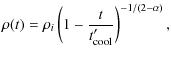
Iwasaki & Tsuribe (2008) (hereafter IT08) have recently found a family of self-similar (S-S) solutions describing the dynamical condensation of a radiative gas layer where the cooling rate dominates the heating rate. This S-S solution assumed that the net cooling rate is a power-law function and that the heating rate is explicitly neglected. Although it is still too ideal, they are expected to be a good nonlinear one-dimensional model at least in the phase during the transition from WNM to CNM. In this paper, we adopt the S-S solutions as a more realistic unsteady unperturbed state than those in previous works. We perform linear analysis of the S-S solutions against fluctuations perpendicular, as well as parallel to, the direction of the condensation. By performing the linear analysis, we will have some useful insights when and how the cooling layer fragments. Since we focus on the above S-S unperturbed state, the nonlinear thin shell instability, Kelvin-Helmholtz instability, and the corrugation instability are beyond the scope of this paper.
In Sect. 2, we formulate basic equations using a zooming coordinate. Perturbation equations are derived for the linear analysis, with a brief review of the S-S solutions. In Sect. 3, we investigate the stability of the S-S solutions taking only those fluctuations into account that are parallel to the direction of the condensation. In Sect. 4, we consider the fluctuations that are both perpendicular and parallel to the direction of the condensation. In Sect. 5, we discuss the astrophysical implication of the linear analysis and effects of the thermal conduction. Our study is summarized in Sect. 6.
2 Formulation
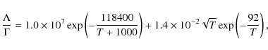
We consider a dynamically condensing radiative gas layer where the cooling rate dominates the heating rate. The following formula is adopted as the net cooling rate per unit volume and time: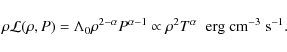
In ISM, in the temperature range of
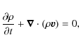
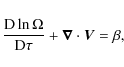
Basic equations for a radiative gas are
the continuity equation,
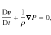
the equation of motion,
and the entropy equation,
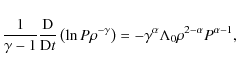
where
We take the x-axis as the direction of
the condensation driven by the cooling and
y-axis as the transverse direction.
Since the S-S solutions are time-dependent, it
is difficult to perform linear analysis
in the ordinary Cartesian coordinate, (t,x,y).
Bouquet et al. (1985) introduced a zooming coordinate
where S-S solutions appear to be stationary
(also see Hanawa & Matsumoto 1999).
We introduce the similar zooming coordinate
since this transformation makes stability analysis easier as follows:
where
respectively, where
and
with
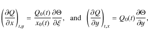
In the zooming coordinate,
the basic Eqs. (2)-(4) are rewritten as
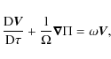
and
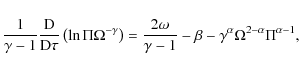
respectively, where the operators of time and spatial derivative are defined by
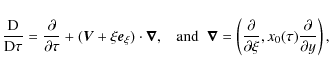
respectively, where
We apply the zooming transformation only in the x-direction but not in the y-direction. This is because the gas contracts along x-axis but not along y-axis in the unperturbed state. In the ordinary coordinate, the transverse scale of the perturbation is expected to be constant with time. However, if the zooming transformation is also applied in the y-direction, the transverse scale of the perturbation decreases with time in the ordinary coordinate, although the unperturbed gas does not contract along the y-axis. Therefore, we apply the zooming transformation only in the x-direction.
2.1 Review of self-similar solutions
In the zooming coordinate, steady state solutions correspond to S-S solutions that were derived in IT08. In this section, physical properties of the S-S solutions are reviewed briefly.The S-S solutions are specified by two parameters, ![]() and
and ![]() .
For convenience, instead of
.
For convenience, instead of ![]() ,
we can use a parameter
,
we can use a parameter ![]() ,
which
is given by
,
which
is given by
|
(14) |
Using these parameters (
respectively, where
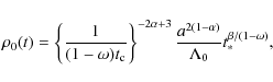
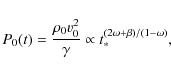
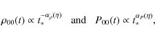
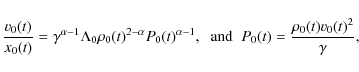
The S-S solutions include two asymptotic solutions.
For ![]() ,
the time dependences of the central density and pressure are
given by
,
the time dependences of the central density and pressure are
given by
|
(16) |
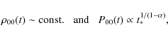
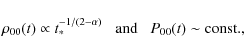
respectively. This time evolution indicates the isochoric mode. For
|
(17) |
respectively. This time evolution corresponds to the isobaric mode. Our S-S solutions exist between the two limits,
|
(18) |
Therefore, the S-S solutions for
2.2 Perturbation equations
Perturbation on the S-S solutions is considered. Perturbed variables are defined by
where subscript ``0'' indicates the unperturbed state.
As the perturbation, we consider the following Fourier mode with respect to y,
and k indicates the wave number of the plane wave that propagates along y-direction. Substituting Eqs. (19) and (20) into Eqs. (10)-(12) and linearizing, we get the following perturbation equations:
and
where
![]() ,
,
|
(25) |
The time-dependent factors remain in the form of
![\begin{figure}
\par\includegraphics[width=12cm,clip]{12806fg1.eps}
\end{figure}](/articles/aa/full_html/2009/47/aa12806-09/img89.png)
|
Figure 1:
Growth rate, |
| Open with DEXTER | |
3 Perturbation for k = 0
In this section, we consider the perturbation parallel to the condensation, or for
the case with k=0.
In this case, since the time-dependent factor,
![]() ,
vanishes,
the perturbed variables can be expanded in the Fourier mode with respect to
,
vanishes,
the perturbed variables can be expanded in the Fourier mode with respect to ![]() as
as
By Eq. (26), the time evolution of the perturbations is given by
Substituting Eq. (26) into the perturbation Eqs. (21)-(24), one obtains the following ordinary differential equations:
where the detailed expression of Aij is shown in Appendix B. Equations (28) are solved as a boundary- and eigenvalue problem.
3.1 Boundary conditions
We impose the boundary conditions at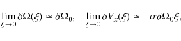
and
where
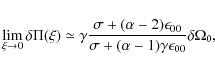
The boundary conditions at the critical point,
![]() ,
are obtained
from Eqs. (28).
At
,
are obtained
from Eqs. (28).
At
![]() ,
the denominator of the righthand side becomes zero.
To obtain a regular solution from
,
the denominator of the righthand side becomes zero.
To obtain a regular solution from ![]() to
to
![]() ,
the numerator of the righthand side should vanish.
Therefore, the boundary conditions are given by the following three equations,
,
the numerator of the righthand side should vanish.
Therefore, the boundary conditions are given by the following three equations,
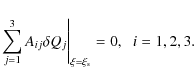
The above three equations give only one independent condition.
3.2 Numerical method
Solutions of Eqs. (28) have three integration constants. Therefore, if we set two constantsWe can set
![]() without loss of generality.
For a given
without loss of generality.
For a given ![]() ,
we integrate Eqs. (28) from
,
we integrate Eqs. (28) from ![]() to
the critical point,
to
the critical point,
![]() ,
using a fourth-order Runge-Kutta method.
Eigenvalue,
,
using a fourth-order Runge-Kutta method.
Eigenvalue, ![]() ,
is modified until the perturbed variables satisfy
the boundary condition at
,
is modified until the perturbed variables satisfy
the boundary condition at
![]() using the Newton-Raphson method.
After that, we integrate Eqs. (28) up to
using the Newton-Raphson method.
After that, we integrate Eqs. (28) up to ![]() .
.
3.3 Results
Figure 1 shows the dependence of growth rate,4 Perturbation with k  0
0
For 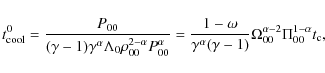
|
(32) |
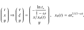
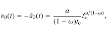
where superscript ``0'' indicates the value at t=0. Therefore, using
Using Eqs. (6) and (7), at t=0, the sound speed at the centre is given by
|
(34) |
Therefore, x0(0) is given by
Using Eq. (33), Eq. (35) can be written as
|
(36) |
where
where
4.1 Static approximation
Before we present the fully time-dependent numerical calculation
in Sect. 4.2,
we at first consider a special case in which the time evolutions of the unperturbed
S-S solutions are slower than the growth of perturbation.
In this situation, the time evolution of the unperturbed state
is negligible during the growth of the perturbations.
Therefore, we set x0 to be a constant in Eqs. (21)-(24).
This approximation is also valid for ![]() where the term,
where the term, ![]() ,
is negligibly small
in Eqs. (21)-(24).
We use the Fourier mode as
,
is negligibly small
in Eqs. (21)-(24).
We use the Fourier mode as
The condition under which the static approximation is valid is given by
where the definition of
where the detailed expression of Aij is shown in Appendix B.
We impose the boundary conditions at ![]() and
and
![]() .
Since we are interested in the fragmentation of the cooling layer,
only the even mode is investigated.
For the even mode,
the perturbed variable should have the following asymptotic forms in
.
Since we are interested in the fragmentation of the cooling layer,
only the even mode is investigated.
For the even mode,
the perturbed variable should have the following asymptotic forms in ![]() :
:
Substituting Eqs. (41) into Eqs. (40), we obtain the following relations:
and
The boundary condition at
Figure 2 shows an approximate dispersion relation
for
![]() with (a)
with (a) ![]() ,
(b) 0.75, and (c) 0.10.
In Fig. 2, one can see several branches labelled by numbers.
The most unstable branch is labelled by (1) for large
,
(b) 0.75, and (c) 0.10.
In Fig. 2, one can see several branches labelled by numbers.
The most unstable branch is labelled by (1) for large ![]() limit, and (2) for small
limit, and (2) for small ![]() limit.
Each branch is explained below.
limit.
Each branch is explained below.
![\begin{figure}
\par\includegraphics[width=6cm,clip]{12806fg2a.eps} \vspace*{2mm}...
...ps} \vspace*{2mm}
\includegraphics[width=6cm,clip]{12806fg2c.eps}
\end{figure}](/articles/aa/full_html/2009/47/aa12806-09/img146.png)
|
Figure 2:
Approximate dispersion relations for
|
| Open with DEXTER | |
| Figure 3:
Eigenfunctions for |
|
| Open with DEXTER | |
(1) The isobaric mode
![\begin{figure}
\par\includegraphics[width=12cm,clip]{12806fg4.eps}
\end{figure}](/articles/aa/full_html/2009/47/aa12806-09/img148.png)
|
Figure 4:
Growth rate as a function of
|
| Open with DEXTER | |
The branch (1) corresponds to the most unstable mode for
![]() ,
or
,
or
![]() .
Since
.
Since
![]() ,
the sound wave can travel the wave length of the perturbation many times
during the runaway cooling of the unperturbed state.
Therefore, the perturbation is expected to grow in pressure
equilibrium with its surroundings,
and the mode corresponds to the isobaric mode.
An example of eigenfunctions
,
the sound wave can travel the wave length of the perturbation many times
during the runaway cooling of the unperturbed state.
Therefore, the perturbation is expected to grow in pressure
equilibrium with its surroundings,
and the mode corresponds to the isobaric mode.
An example of eigenfunctions
![]() for the branch (1)
is shown in Fig. 3 for
for the branch (1)
is shown in Fig. 3 for ![]() and
and
![]() .
In Fig. 3, it is clearly seen that
.
In Fig. 3, it is clearly seen that
![]() .
This behaviour also implies the isobaric mode.
.
This behaviour also implies the isobaric mode.
The growth rate in the isobaric mode can also be derived analytically
by considering the evolution of a fluid element at the centre. The fluid element
is assumed to have an isobaric fluctuation,
![]() and
P=P00(t).
From Eq. (4),
the following perturbation equation is obtained:
and
P=P00(t).
From Eq. (4),
the following perturbation equation is obtained:
From Eqs. (8) and (9), we have
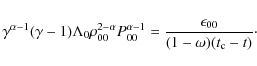
Using Eq. (47), Eq. (46) is rewritten as
Equation (48) can be integrated to give
|
(49) |
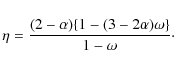
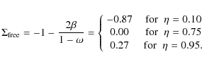
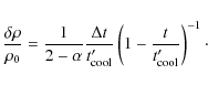
Therefore, the growth rate in isobaric mode is given by
![$\displaystyle \left[ 1-\frac{2-\alpha}{\gamma(1-\alpha)} \right]\eta
+ \frac{2-...
...for}\;\;\eta=0.75 \\
1.04 & \;\;{\rm for}\;\;\eta=0.95. \\
\end{array}\right.$](/articles/aa/full_html/2009/47/aa12806-09/img161.png)
In Fig. 2b, the eigen-value,
For the density perturbation to grow sufficiently during the runaway cooling,
it must grow faster than the condensation of the cooling layer.
This condition can be expressed by
![]() .
Figure 4 shows
.
Figure 4 shows
![]() ,
,
![]() and
and ![]() as a function of
as a function of ![]() for (a)
for (a)
![]() and (b) 0.8.
From Fig. 4, it is found that
and (b) 0.8.
From Fig. 4, it is found that
![]() is greater than
is greater than
![]() for all
for all ![]() .
For other
.
For other ![]() ,
we can investigate analytically as follows:
subtracting
,
we can investigate analytically as follows:
subtracting
![]() from
from
![]() ,
one obtains
,
one obtains
| |
= | ![$\displaystyle \left[ 1-\frac{2-\alpha}{\gamma(1-\alpha)} - \frac{1}{2-\alpha}\right]\eta
+ \frac{2-\alpha}{\gamma(1-\alpha)}$](/articles/aa/full_html/2009/47/aa12806-09/img166.png)
|
|
| (51) |
Therefore, for
| Figure 5: Schematic picture of the noninteractive mode. |
|
| Open with DEXTER | |
(2) The noninteractive mode
Branch (2) corresponds to the most unstable mode for
![]() .
Because the wave length is larger than the cooling length, each part evolves independently
according to the S-S solutions. We call this branch the noninteractive mode.
Figure 5 shows the schematic picture of the noninteractive mode.
In Fig. 5, similarity variables have an initial fluctuation.
For example, we consider two different regions, ``A'' and ``B'', where
.
Because the wave length is larger than the cooling length, each part evolves independently
according to the S-S solutions. We call this branch the noninteractive mode.
Figure 5 shows the schematic picture of the noninteractive mode.
In Fig. 5, similarity variables have an initial fluctuation.
For example, we consider two different regions, ``A'' and ``B'', where
![]() and
and
![]() .
Due to the difference of
.
Due to the difference of
![]() ,
the regions ``A'' and ``B'' have different collapse time,
,
the regions ``A'' and ``B'' have different collapse time,
![]() and
and ![]() ,
respectively.
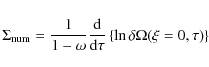
Omitting any terms that do not grow, we find the time evolution of difference,
,
respectively.
Omitting any terms that do not grow, we find the time evolution of difference,
![]() ,
to be
,
to be
![\begin{displaymath}\frac{\Delta \rho}{\rho_0(t)} =
- \Omega(\xi)\Delta t\left[ \...
...\ln\Omega}{{\rm d}\ln\xi} \right]
\frac{1}{t_{\rm c}-t}{\cdot}
\end{displaymath}](/articles/aa/full_html/2009/47/aa12806-09/img175.png)
|
(52) |
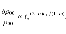
Therefore, in the zooming coordinate, the density perturbation grows as
| (53) |
which is independent of
We investigate whether the noninteractive mode grows sufficiently during the runaway cooling or not.
First, we consider the case with
![]() .
Since the perturbation grows isobarically,
.
Since the perturbation grows isobarically,
![]() is compared to
is compared to
![]() .
From Fig. 4, it is seen that the growth rate,
.
From Fig. 4, it is seen that the growth rate,
![]() ,
is
higher than
,
is
higher than
![]() for all
for all
![]() and 0.86
for
and 0.86
for
![]() and 0.8, respectively.
Therefore, the noninteractive mode can grow sufficiently.
Next, we consider the cooling layer with
and 0.8, respectively.
Therefore, the noninteractive mode can grow sufficiently.
Next, we consider the cooling layer with
![]() .
In this layer, since the perturbation grows
isochorically,
.
In this layer, since the perturbation grows
isochorically,
![]() is compared to
is compared to
![]() .
Analytically, it is found that the pressure perturbation
can only grow for
.
Analytically, it is found that the pressure perturbation
can only grow for
![]() .
.
Koyama & Inutsuka (2000) performed a linear analysis of a spatially uniform and isobarically cooling gas in their appendix. However, they did not find the noninteractive mode. This is because they fixed the collapse time to be spatially constant, and it was assumed not to be influenced by perturbation. Burkert & Lin (2000) performed linear analysis of a spatially uniform and isochorically cooling gas by taking account of the time evolution of the unperturbed state. They showed that a perturbation cannot grow in the condition for long wave length limit. Our result is consistent with theirs.
| Figure 6:
Growth rate obtained by results of
numerical linear analysis for |
|
| Open with DEXTER | |
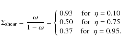
(3) The shear mode
For
![]() ,
there is a solution where physical variables are very small except for
,
there is a solution where physical variables are very small except for
![]() which is spatially constant, and the eigenvalue is
which is spatially constant, and the eigenvalue is
![]() .
The similar mode was found by McNamara (1993), who investigated TI of a uniform granular medium.
McNamara (1993) called this mode the shear mode.
The growth rate is given by
.
The similar mode was found by McNamara (1993), who investigated TI of a uniform granular medium.
McNamara (1993) called this mode the shear mode.
The growth rate is given by
In Fig. 2, it is seen that each growth rate in branch (3) has the corresponding value of
(4) The free-streaming mode
For large ![]() ,
there is another mode in which
the velocity perturbation in the x-direction is
much greater than that in the y-direction,
,
there is another mode in which
the velocity perturbation in the x-direction is
much greater than that in the y-direction,
![]() .
We call this mode the free-streaming mode.
From Eq. (45) with
.
We call this mode the free-streaming mode.
From Eq. (45) with
![]() ,
we obtain
,
we obtain
|
(55) |
In the free-streaming mode, the growth of the velocity perturbation in the x-direction is hampered by the pressure gradient of the unperturbed state. Therefore, the growth rate is less than the shear mode.
(5) ![]() mode
mode
The growth rate in this branch for
![]() coincides with the case with k=0, which is obtained in
Sect. 3.
coincides with the case with k=0, which is obtained in
Sect. 3.
4.2 Linear analysis considering the time evolution of 
The static approximation is valid only if We impose the boundary conditions at ![]() and
and ![]() .
The even mode is set as the boundary condition at
.
The even mode is set as the boundary condition at ![]() .
The free boundary condition is set at
.
The free boundary condition is set at ![]() ,
but it does not influence the inner region
since the gas flows out supersonically
from the outer boundary of the zooming coordinate.
As an initial state, we adopt the eigenfunction
of the isobaric mode for
,
but it does not influence the inner region
since the gas flows out supersonically
from the outer boundary of the zooming coordinate.
As an initial state, we adopt the eigenfunction
of the isobaric mode for ![]() which
is obtained in Sect. 4.1.
which
is obtained in Sect. 4.1.
By solving Eqs. (21)-(24),
a time evolution of
![]() is obtained.
During the calculation, the growth rate at
is obtained.
During the calculation, the growth rate at ![]() is evaluated by
is evaluated by
|
(56) |
at each instant of time. For comparison with the result of the static approximation, we focus on a relation between
5 Discussion
5.1 Astrophysical implication
In this section, we estimate the fragmentation time of the cooling layer formed by a collision of WNM. We consider a head-on collision between two thermally equilibrium gases in which density and pressure are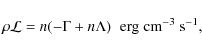
|
(57) |
where

|
(58) |
|
(59) |
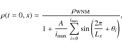
where n is the number density of the gas. We perform numerical calculation using the one-dimensional Lagrangian Godunov scheme (van Leer 1997) between x=0 and x=Lx = 3.26 pc. At x=0 and x=Lx, we adopt the reflecting and free boundary conditions, respectively. As the initial condition, we add the following density fluctuation:
|
(60) |
where we set
![\begin{figure}
\par\includegraphics[width=6cm,clip]{12806fg7.eps}
\end{figure}](/articles/aa/full_html/2009/47/aa12806-09/img213.png)
|
Figure 7: Evolutionary track of the gas at the centre after the head-on collision (the thick solid line). The ordinate and abscissa axes indicate the pressure and the number density, respectively. The thin solid line indicates the thermally equilibrium curve. The filled circle represents the gas at the preshock region. |
| Open with DEXTER | |
![\begin{figure}
\par\includegraphics[width=6cm,clip]{12806fg8.eps}
\end{figure}](/articles/aa/full_html/2009/47/aa12806-09/img214.png)
|
Figure 8:
Time evolution of
|
| Open with DEXTER | |
![\begin{figure}
\par\includegraphics[width=12cm,clip]{12806fg9.eps}
\end{figure}](/articles/aa/full_html/2009/47/aa12806-09/img215.png)
|
Figure 9:
Time evolution of a) the number density and b) the temperature,
respectively.
The rescaled c) number density,
|
| Open with DEXTER | |
Figure 7 shows the evolutionary track of the gas
at the centre, x=0.
Due to the shock compression, the temperature of gas
increases suddenly, and the postshock region enters the thermally
unstable phase from the initial stable
state. The TI leads to the cooling layer condensing in a runaway fashion.
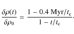
The cooling length in Fig. 8 rapidly decreases with time until
it reaches minimum value
![]() pc at t=0.917 Myr.
During runaway cooling, the gas condenses isobarically until it reaches
the stable CNM phase, although some pressure oscillation is seen in Fig. 7.
We focus on the property of this runaway condensing layer. First
we evaluate
pc at t=0.917 Myr.
During runaway cooling, the gas condenses isobarically until it reaches
the stable CNM phase, although some pressure oscillation is seen in Fig. 7.
We focus on the property of this runaway condensing layer. First
we evaluate
![]() ,
which is defined by
,
which is defined by
|
(61) |
at each instant of time. Figure 8 shows the time evolution of
Figures 9 show
the time evolutions of the distributions of (a) the number density and (b) the temperature
at t= 0.72, 0.80, 0.88, and 0.90 Myr, respectively.
The rescaled number density
![]() and temperature,
and temperature,
![]() are shown in
Figs. 9c and 9d
as a function of rescaled coordinate,
are shown in
Figs. 9c and 9d
as a function of rescaled coordinate,
![]() ,
where
,
where ![]() ,
,
![]() ,
and
,
and ![]() are set to 0.915 Myr, 0.98, and 0.61, respectively.
From Figs. 9c and 9d, it is clearly seen that the
S-S solution
are set to 0.915 Myr, 0.98, and 0.61, respectively.
From Figs. 9c and 9d, it is clearly seen that the
S-S solution
![]() describes
the results of the numerical calculation well.
There are two reasons they are described by the S-S solution well.
One is that
describes
the results of the numerical calculation well.
There are two reasons they are described by the S-S solution well.
One is that
![]() is almost constant, and
the cooling function is approximated well by Eq. (1) during the runaway condensation.
The other reason relates to the stability of S-S solutions.
The one-dimensional calculation solves the evolution only in the direction parallel to the condensation.
From the linear analysis in Sect. 3,
such a perturbation with k=0 cannot grow enough during the
runaway condensation.
That is why the S-S solution is realized even though the density is initially fluctuated.
is almost constant, and
the cooling function is approximated well by Eq. (1) during the runaway condensation.
The other reason relates to the stability of S-S solutions.
The one-dimensional calculation solves the evolution only in the direction parallel to the condensation.
From the linear analysis in Sect. 3,
such a perturbation with k=0 cannot grow enough during the
runaway condensation.
That is why the S-S solution is realized even though the density is initially fluctuated.
However, the result is expected to be qualitatively different if the perturbation with ![]() exists.
The perturbation with
exists.
The perturbation with ![]() on the isobarically runaway condensing layer
grows as
on the isobarically runaway condensing layer
grows as
![]() (see Sect. 4). The growth rate is independent of wave numbers.
From Figs. 8 and 9,
the gas evolves obeying the S-S solution between t= 0.4 and 0.9 Myr.
If the layer has a perturbation (
(see Sect. 4). The growth rate is independent of wave numbers.
From Figs. 8 and 9,
the gas evolves obeying the S-S solution between t= 0.4 and 0.9 Myr.
If the layer has a perturbation (![]() )
with
amplitude
)
with
amplitude
![]() at
at
![]() ,
the perturbation grows as
,
the perturbation grows as
|
(62) |
The epochs when the perturbation grows by a factor of 10 and 100 are t= 0.86 and 0.91 Myr, respectively. At 0.86 Myr, the central number density is still as low as 38 cm-3. Therefore, the condensing layer is expected to fragment quickly, and CNM clumps will form.
Inoue & Inutsuka (2008) investigated TI in a shock compressed region formed by WNM-WNM collision using two-dimensional, two-fluid magnetohydrodynamical simulation. The initial condition there is the same as that in our one-dimensional simulation except for the dimension and the way to add density fluctuation in the WNM. Our linear analysis is applicable to the gas evolution before CNM clouds form in their unmagnetized case. In the initial stage of their simulation, in the postshock region, thermally unstable gas initially condenses in a layer structure. Around t=0.5 Myr when the region of the highest density reaches CNM stable state, both small CNM cloudlets and filamentary CNM clouds are generated (Inoue 2009, priv. comm.). According to our linear analysis, an isobarically condensing gas layer is expected to split into fragments that have a variety of lengths in the transverse direction. Therefore, our linear analysis agrees with their simulation qualitatively.
After the first CNM clouds formation, the mass of these CNM clouds continues to increase by the accretion of unstable gas by the shocks. Moreover, some CNM clouds coalesce into larger clouds and others fragment into smaller ones by the turbulent flow (Inoue 2009, priv. comm.). Therefore, the size and mass of CNM clouds varies with time. To understand this phase, which is beyond the scope of this paper, a statistical approach is probably needed. A statistical theory has been proposed by Hennebelle & Audit (2007) using Press-Schechter formalism (Press & Schechter 1974), assuming that the CNM clumps are generated from density fluctuations within WNM whose power spectrum is assumed to be Kolmogorov.
Comparing timescales, Heitsch et al. (2008) discuss the effect of TI, the nonlinear thin-shell instability, Kelvin-Helmholtz instability, and gravitational instability in various densities, temperatures, and scales of fluctuations. In their paper, it is assumed that the gas is unstable only if the scale of the fluctuation is smaller than the sound crossing scale. However, from our linear analysis, perturbations can grow regardless of their scales as long as they are flat rather than spherical.
5.2 The growth rate for

Although the linear analysis on the S-S cooling layer is limited for 5.2.1 The isobaric mode
For the case with small wave length, perturbation is expected to grow isobarically. By comparison of our results with previous studies in the literature, it is found that the growth rate in the isobaric mode is independent of the global structure of the unperturbed state. Therefore, from local arguments, the growth rate in the isobaric mode of the gas withAs an unperturbed state, we adopt a cooling gas element whose scale is assumed to be much smaller than the cooling length. In this case, the element cools isobarically. From Eq. (4), the time evolution of the unperturbed gas is given by
where ![]() and Pi represent the initial density and pressure, respectively.
In the above unperturbed state, we consider the following isobaric perturbation:
and Pi represent the initial density and pressure, respectively.
In the above unperturbed state, we consider the following isobaric perturbation:
| (64) |
and
| P = P0, | (65) |
where subscript ``0'' indicates the unperturbed state, and
Using Eq. (63), Eq. (66) is rewritten as
Equation (67) is easily integrated to give
Comparing Eq. (68) with Eq. (63), one can see that the perturbation grows more slowly than the unperturbed state for
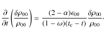
5.2.2 The noninteractive mode
A cooling layer that evolves isobarically is considered. The time evolution of the central density is the same as Eq. (63). When the scale of perturbation perpendicular to the condensation is too large to interact with other regions, each region evolves independently. Here, we focus on the time evolution of density perturbation at the centre (x=0). Initial fluctuation of the central density,
Linearizing Eq. (69) with omitting terms that do not grow, we have
Comparing Eq. (70) with Eq. (63), we can see that the perturbation grows more slowly than the unperturbed state for
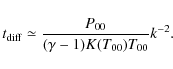
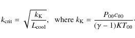
5.3 Effects of thermal conduction
In this paper, the thermal conduction is neglected for simplicity. However, for large wave number, the thermal conduction is expected to stabilize TI in the cooling layer (Field 1965). Therefore, there is a critical wave number,First, we evaluate
![]() using an order estimation.
Using the characteristic time scale of the thermal conduction,
using an order estimation.
Using the characteristic time scale of the thermal conduction,
![]() ,
the diffusion equation is given by
,
the diffusion equation is given by
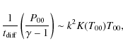
where K is the thermal conduction coefficient. From Eq. (71), the diffusion timescale is given by
From Eq. (72), one can see that the diffusion timescale is small for large wave number. If
Field (1965) derived similar critical wave number to Eq. (73). Since the unperturbed state is time dependent,
For
Figure 8 shows the time evolution of
the critical wave length,
![]() .
In Sect. 5.1, the time evolution of the condensing layer can be
described by the S-S solution with (
.
In Sect. 5.1, the time evolution of the condensing layer can be
described by the S-S solution with (
![]() ,
,
![]() ).
In Fig. 8, we see that
).
In Fig. 8, we see that
![]() decreases
with time during the runaway condensation.
Figure 8 also shows that
decreases
with time during the runaway condensation.
Figure 8 also shows that
![]() ,
or
,
or
![]() .
This means that the effect of thermal conduction on the dispersion relation
(Fig. 6) always appears in the isobaric regime during the runaway condensation.
.
This means that the effect of thermal conduction on the dispersion relation
(Fig. 6) always appears in the isobaric regime during the runaway condensation.
6 Summary
In this paper, we have investigated the stability of S-S solutions describing the runaway cooling of a radiative gas by linear analysis. The results of our investigation are summarized as follows,- 1.
- For the case with perturbation only parallel to the flow (k=0), the S-S solutions are unstable. However, the growth rate is too low to become nonlinear during the runaway cooling. Actually, the S-S solutions are realized in one-dimensional hydrodynamical calculations in IT08 and in Sect. 5.1 in this paper.
- 2.
- For the case with transverse perturbation (
 ),
there are several unstable modes in the S-S solutions.
The most unstable modes are the isobaric mode for
),
there are several unstable modes in the S-S solutions.
The most unstable modes are the isobaric mode for  and
the noninteractive mode for
and
the noninteractive mode for  .
In the isobaric mode, the perturbation grows in pressure
equilibrium with its surroundings.
On the other hand, the noninteractive mode is originated from
each region in the layer condensing independently.
Under a static approximation, we derive the approximated dispersion relation.
The results of direct numerical integration of the time evolution
agree with those using the static approximation.
.
In the isobaric mode, the perturbation grows in pressure
equilibrium with its surroundings.
On the other hand, the noninteractive mode is originated from
each region in the layer condensing independently.
Under a static approximation, we derive the approximated dispersion relation.
The results of direct numerical integration of the time evolution
agree with those using the static approximation.
- 3.
- The S-S solutions for
 are unstable for any wavelength.
Especially, if the unperturbed state is isobaric, the growth rate
is independent of wave number. Therefore, fluctuations in various scales
grow simultaneously, and the gas layer is expected to split
into fragments with various scales.
The S-S solutions for
are unstable for any wavelength.
Especially, if the unperturbed state is isobaric, the growth rate
is independent of wave number. Therefore, fluctuations in various scales
grow simultaneously, and the gas layer is expected to split
into fragments with various scales.
The S-S solutions for
 are only unstable in the
isobaric mode.
are only unstable in the
isobaric mode.
We would like to thank Tsuyoshi Inoue for valuable discussions. We also would like to thank the anonymous referee for valuable comments and suggestions that improved this paper significantly. K.I. is supported by grants-in-aid for JSPS Fellow (21-1979).
Appendix A: Supplements for derivation of basic equations in the zooming coordinate
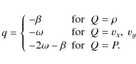
Here, we present preparation for derivation of basic Eqs. (10)-(12) in the zooming coordinate given by Eq. (5). In the zooming coordinate, the physical variables, Q(t,x,y), are given by the following unified form: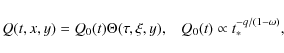
|
(A.1) |
where Q(t,x,y) corresponds to
|
(A.2) |
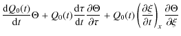
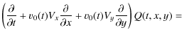
The temporal and spatial derivatives of Q(t,x,y) in the ordinary coordinate can be expressed in the zooming coordinate as

![$\displaystyle \frac{v_0(t)}{x_0(t)}Q_0(t)
\left[ q \Theta
+ \frac{\partial \Theta}{\partial \tau}
+ \xi\frac{\partial \Theta}{\partial \xi} \right],$](/articles/aa/full_html/2009/47/aa12806-09/img271.png)
respectively, where we use
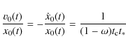
from Eq. (7). Using Eqs. (A.3) and (A.4), the Lagrangian time derivative of Q is given by
![$\displaystyle ~\frac{v_0(t)}{x_0(t)}Q_0(t) \left[ q
+ \frac{\partial}{\partial ...
...rtial \xi}
+ V_y x_0(t)\frac{\partial }{\partial y} \right]
\Theta(\tau,\xi,y).$](/articles/aa/full_html/2009/47/aa12806-09/img275.png)
|
(A.7) |
basic Eqs. (10)-(12) are derived in the zooming coordinate.
Appendix B: Detailed expression of A

In this appendix, we provide the detail expression of Aik as
|
(B.1) |
|
(B.2) |
![\begin{displaymath}A_{13}= \frac{X_0^2}{\gamma}
\left[ (\ln\Pi_0)' - \frac{\sigma + (\alpha-1)\gamma\epsilon_0}{V_0} \right],
\end{displaymath}](/articles/aa/full_html/2009/47/aa12806-09/img280.png)
|
(B.3) |
| A14= - kx0(t)V0, | (B.4) |

|
(B.5) |
|
(B.6) |
| A23= -V0A14, | (B.7) |
| A24= kx0(t)X02, | (B.8) |
|
(B.9) |
|
(B.10) |
|
(B.11) |
| (B.12) |
| A41= 0, | (B.13) |
| A42= 0, | (B.14) |
|
(B.15) |
and
|
(B.16) |
References
- Audit, E., & Hennebelle, P. 2005, A&A, 433, 1 [NASA ADS] [EDP Sciences] [CrossRef]
- Balbus, S. A. 1986, ApJ, 303, L79 [NASA ADS] [CrossRef]
- Bouquet, S., Feix, R., & Fijalkow, E. 1985, ApJ, 293, 494 [NASA ADS] [CrossRef]
- Burkert, A., & Lin, D. N. C. 2000, ApJ, 537, 270 [NASA ADS] [CrossRef]
- Dalgarno, A., & MaCray, R. 1972, ARA&A, 10, 375 [NASA ADS] [CrossRef]
- Field, G. B. 1965, ApJ, 142, 531 [NASA ADS] [CrossRef]
- Field, G. B., Goldsmith, D. W., & Habing, H. J. 1969, ApJ, 155, L149 [NASA ADS] [CrossRef]
- Hanawa, T., & Matsumoto, T. 1999, ApJ, 521, 703 [NASA ADS] [CrossRef]
- Heitsch, F., Slyz, A. D., Devriendt, J. E. G., Hartmann, L. W., & Burkert, A. 2006, ApJ, 648, 1052 [NASA ADS] [CrossRef]
- Heitsch, F., Hartmann, L. W., & Burkert, A. 2008, ApJ, 683, 786 [NASA ADS] [CrossRef]
- Hennebelle, P., & Audit, E. 2007, A&A, 465, 431 [NASA ADS] [EDP Sciences] [CrossRef]
- Hennebelle, P., & Passot, T. 2006, A&A, 448, 1083 [NASA ADS] [EDP Sciences] [CrossRef]
- Inoue, T., & Inutsuka, S. 2008, ApJ, 687, 303 [NASA ADS] [CrossRef]
- Inoue, T., Inutsuka, S., & Koyama, H. 2006, ApJ, 652, 1331 [NASA ADS] [CrossRef]
- Iwasaki, K., & Tsuribe, T. 2008, MNRAS, 384, 1554 [NASA ADS] [CrossRef]
- Koyama, H., & Inutsuka, S. 2000, ApJ, 321, 980 [NASA ADS] [CrossRef]
- Koyama, H., & Inutsuka, S. 2002, ApJ, 564, L97 [NASA ADS] [CrossRef]
- McNamara, S. 1993, Phys. Fluids A, 5, 3056 [NASA ADS] [CrossRef]
- Parker, E. N. 1953, ApJ, 117, 431 [NASA ADS] [CrossRef]
- Press, W., & Schechter, P. 1974, ApJ, 187, 425 [NASA ADS] [CrossRef]
- Schwarz, J., McCray, R., & Stein, R. F. 1972, ApJ, 175, 673 [NASA ADS] [CrossRef]
- Sutherland, R. S., & Dopita, M. A. 1993, ApJS, 88, 253 [NASA ADS] [CrossRef]
- van Leer, B. 1997, J. Comput. Phys., 135, 229 [NASA ADS] [CrossRef]
- Vazquez-Semadeni, E., Gomez, G. C., Jappsen, A. K., et al. 2007, ApJ, 657, 870 [NASA ADS] [CrossRef]
- Vishniac, E. 1994, ApJ, 428, 186 [NASA ADS] [CrossRef]
- Wolfire, M. G., Hollenbach, D., McKee, C. F., Tielens, A. G. G. M., & Bakes, E. L. O. 1995, ApJ, 443, 152 [NASA ADS] [CrossRef]
- Wolfire, M. G., McKee, C. F., Hollenbach, D., & Tielens, A. G. G. M. 2003, ApJ, 587, 278 [NASA ADS] [CrossRef]
All Figures
|
|
Figure 1:
Growth rate, |
| Open with DEXTER | |
| In the text | |
|
|
Figure 2:
Approximate dispersion relations for
|
| Open with DEXTER | |
| In the text | |
| |
Figure 3:
Eigenfunctions for |
| Open with DEXTER | |
| In the text | |
|
|
Figure 4:
Growth rate as a function of
|
| Open with DEXTER | |
| In the text | |
| |
Figure 5: Schematic picture of the noninteractive mode. |
| Open with DEXTER | |
| In the text | |
| |
Figure 6:
Growth rate obtained by results of
numerical linear analysis for |
| Open with DEXTER | |
| In the text | |
|
|
Figure 7: Evolutionary track of the gas at the centre after the head-on collision (the thick solid line). The ordinate and abscissa axes indicate the pressure and the number density, respectively. The thin solid line indicates the thermally equilibrium curve. The filled circle represents the gas at the preshock region. |
| Open with DEXTER | |
| In the text | |
|
|
Figure 8:
Time evolution of
|
| Open with DEXTER | |
| In the text | |
|
|
Figure 9:
Time evolution of a) the number density and b) the temperature,
respectively.
The rescaled c) number density,
|
| Open with DEXTER | |
| In the text | |
Copyright ESO 2009
Current usage metrics show cumulative count of Article Views (full-text article views including HTML views, PDF and ePub downloads, according to the available data) and Abstracts Views on Vision4Press platform.
Data correspond to usage on the plateform after 2015. The current usage metrics is available 48-96 hours after online publication and is updated daily on week days.
Initial download of the metrics may take a while.