| Issue |
A&A
Volume 508, Number 2, December III 2009
|
|
|---|---|---|
| Page(s) | 841 - 848 | |
| Section | Stellar structure and evolution | |
| DOI | https://doi.org/10.1051/0004-6361/200912642 | |
| Published online | 21 October 2009 | |
A&A 508, 841-848 (2009)
X-ray emission from hydrodynamical simulations in non-LTE wind models
J. Krticka1 - A. Feldmeier2 - L. M. Oskinova2 - J. Kubát3 - W.-R. Hamann2
1 - Ústav teoretické fyziky a astrofyziky, Masarykova univerzita,
Kotlárská 2, 611 37 Brno, Czech Republic
2 -
Institut für Physik und Astronomie, Universität Potsdam,
Karl-Liebknecht-Straße 24/25, 14476 Potsdam-Golm, Germany
3 -
Astronomický ústav, Akademie ved Ceské
republiky, 251 65 Ondrejov, Czech Republic
Received 5 June 2009 / Accepted 9 September 2009
Abstract
Hot stars are sources of X-ray emission originating in their winds.
Although hydrodynamical simulations that are able to predict this X-ray
emission are available, the inclusion of X-rays in stationary wind
models is usually based on simplifying approximations. To improve
this, we use results from time-dependent hydrodynamical simulations of
the line-driven wind instability
(seeded by the base perturbation) to derive the analytical
approximation of X-ray emission in the stellar wind. We use this
approximation in our non-LTE wind models and find that an improved
inclusion of X-rays leads to a better agreement between model
ionization fractions and those derived from observations. Furthermore,
the slope of the
![]() relation
is in better agreement with
observations, however the X-ray luminosity is underestimated by a
factor of three. We propose a possible solution for this discrepancy.
relation
is in better agreement with
observations, however the X-ray luminosity is underestimated by a
factor of three. We propose a possible solution for this discrepancy.
Key words: stars: winds, outflows - stars: mass-loss - stars: early-type - hydrodynamics - X-rays: stars
1 Introduction
Hot-star winds have been traditionally modelled assuming a spherically symmetric, stationary outflow. These assumptions provide a convenient basis for studying different phenomena that may influence the wind structure. The line profiles and wind parameters predicted in this way are in good agreement with those found from observations (e.g., Vink et al. 2001; Krticka 2006; Pauldrach et al. 2001).
However, a stationary approach to hot-star wind modelling was for a long time known to be not fully adequate (Lucy & Solomon 1970). Hydrodynamical simulations show the growth of strong shocks in the wind due to the so-called line-driven instability inherent to radiative driving (Feldmeier et al. 1997a; Owocki et al. 1988). On the other hand, from the observational point of view the inhomogeneities do not imprint a clear signature in hot-star wind spectra in ultraviolet and visible spectral regions, and only a detailed spectral analysis reveals its possible presence (Bouret et al. 2003; Puls et al. 2006; Martins et al. 2005). Consequently, the influence of inhomogeneities (or clumping) on wind spectra has long been neglected. At present it is not clear whether the neglect of wind clumps in the formation of wind line profiles and infrared continua leads to an overestimate of mass-loss rates derived from observations (see Puls et al. 2008a, for a discussion of this problem).
The only clear observable signature of intrinsic wind non-stationarity is the existence of X-ray emission. This emission is directly observable for nearby stars (e.g., Antokhin et al. 2008; Berghöfer et al. 1997) and its existence can be inferred from the influence on the ultraviolet spectrum for those stars for which a direct observation of their X-ray emission is not available (e.g., Bianchi et al. 2004).
The line-driven instability is not the only possible production mechanism of X-rays in hot star winds. Because the winds are highly supersonic, any mechanism which causes wind stream collisions may also lead to X-ray production. Consequently, in hot star binaries the X-rays may originate due to the collisions of winds from individual stars (e.g., Pittard 2009; Prilutskii & Usov 1976; Cooke et al. 1978). The collisions of individual wind streams channeled by the magnetic field may also cause X-ray emission (ud-Doula & Owocki 2002; Babel & Montmerle 1997). The former mechanism is important in binaries and the latter one in stars with a sufficiently strong magnetic field. In this paper we concentrate on a more general mechanism, operating in all radiatively driven stellar winds, i.e., the line-driven instability.
A central observational finding related to the X-ray emission is the dependence of the X-ray luminosity ![]() on the total luminosity L via the approximate relation
on the total luminosity L via the approximate relation
![]() (e.g., Chlebowski et al. 1989). This relationship is still not explained by wind
theory. Assuming a constant X-ray filling factor, Owocki & Cohen (1999) showed that for stars with optically thick winds the observed X-ray luminosity scales with the mass-loss rate as
(e.g., Chlebowski et al. 1989). This relationship is still not explained by wind
theory. Assuming a constant X-ray filling factor, Owocki & Cohen (1999) showed that for stars with optically thick winds the observed X-ray luminosity scales with the mass-loss rate as
![]() ,
and for stars with optically thin winds as
,
and for stars with optically thin winds as
![]() .
As the predicted wind mass-loss rate scales with the stellar luminosity as
.
As the predicted wind mass-loss rate scales with the stellar luminosity as
![]() (Kudritzki & Puls 2000), where
(Kudritzki & Puls 2000), where
![]() for luminuous O stars
for luminuous O stars![]() (e.g., Puls et al. 2008b; Vink et al. 2000; Krticka & Kubát 2009), the predicted slope of the
(e.g., Puls et al. 2008b; Vink et al. 2000; Krticka & Kubát 2009), the predicted slope of the
![]() relation
is steeper than the observed one. This difference may originate in the
radial dependence of the X-ray filling factor (Owocki & Cohen 1999) or may be caused by the dependence of the cooling length on the wind density (Krticka & Kubát 2009). Note also that macroclumping (Oskinova et al. 2006; Feldmeier et al. 2003; Oskinova et al. 2004; Owocki et al. 2004) may lead to a decrease in the effective opacity in the X-ray region and affect the X-ray luminosity.
relation
is steeper than the observed one. This difference may originate in the
radial dependence of the X-ray filling factor (Owocki & Cohen 1999) or may be caused by the dependence of the cooling length on the wind density (Krticka & Kubát 2009). Note also that macroclumping (Oskinova et al. 2006; Feldmeier et al. 2003; Oskinova et al. 2004; Owocki et al. 2004) may lead to a decrease in the effective opacity in the X-ray region and affect the X-ray luminosity.
Although a real hot-star wind should be far from stationary and spherically symmetric (on small scales), the success of wind modelling applying these approximations motivates us to incorporate the inhomogeneities found in time-dependent hydrodynamical simulations into a spherically symmetric, stationary wind model. These models can serve as an efficient tool to study hot-star winds until more elaborate hydrodynamical simulations that consistently take into account the non-LTE effects become available.
There have been earlier attempts to include X-ray emission in non-LTE wind models. They were either based on simplified analytical models (Feldmeier et al. 1997b; Martins et al. 2005), or the X-ray emission was included using ad hoc free parameters (aka the ``filling factor'', e.g., Krticka & Kubát 2009; Martins et al. 2005; MacFarlane et al. 1994) describing the hot wind part. Here we use the results of available hydrodynamical simulations of Feldmeier et al. (1997a) to directly describe the X-ray emission in a compact form and include it in our non-LTE wind models.
2 Hydrodynamical simulations
The hydrodynamical simulations we employ here to estimate the X-ray emission from O stars were performed using the smooth source function method (SSF, Owocki & Puls 1996; Owocki 1991).
This
corresponds roughly to a formal integral of the radiation force using a
pre-specified line source function, here the optically thin source
function,
![]() .
The line-driven instability that is responsible for the formation of
X-ray emitting shocks in the wind is captured by a careful integration
of the line-optical depth with a resolution of three observer-frame
frequency points per line Doppler width and accounting for non-local
couplings in the non-monotonic velocity law of the wind (see Owocki et al. 1988,
for details). The angle integration in the radiative flux is limited to
one single ray which, however, is not the radial ray but hits the star
at
.
The line-driven instability that is responsible for the formation of
X-ray emitting shocks in the wind is captured by a careful integration
of the line-optical depth with a resolution of three observer-frame
frequency points per line Doppler width and accounting for non-local
couplings in the non-monotonic velocity law of the wind (see Owocki et al. 1988,
for details). The angle integration in the radiative flux is limited to
one single ray which, however, is not the radial ray but hits the star
at
![]() .
This accounts with sufficient accuracy for the finite-disk correction factor (Pauldrach et al. 1986) and avoids the critical-point degeneracy of the point-star CAK model (Poe et al. 1990).
.
This accounts with sufficient accuracy for the finite-disk correction factor (Pauldrach et al. 1986) and avoids the critical-point degeneracy of the point-star CAK model (Poe et al. 1990).
To avoid any artificial overestimate of the X-ray production in the wind, special care was taken in the numerical calculation of the line force on the staggered spatial mesh in order to correctly reproduce the line-drag effect (Lucy 1984), which is responsible for a partial reduction of the instability, especially in layers close to the star (Owocki & Rybicki 1985). The pure hydrodynamics part of the code is a standard van Leer solver following standard prescriptions for such a scheme: staggered mesh; operator splitting of advection and source terms; advection terms in a conservative form using van Leer's (1977) monotonic derivative as an optimised compromise between stability and accuracy; Richtmyer artificial viscosity; and non-reflecting boundary conditions (Thompson 1990; Hedstrom 1979; Thompson 1987). The numerical collapse of post-shock radiative cooling zones caused by the strong oscillatory thermal instability (Langer et al. 1981) is prevented by artificially modifying the radiative cooling function below a certain temperature at which X-ray emissivity is still small. Further details can be found in Feldmeier (1995).
As seed perturbations for unstable growth we introduce a turbulent variation of the velocity at the wind base, at a level of roughly one third of the sound speed. This perturbation is obtained from a simple quadrature of the Langevin equation (see Risken 1996) with a coherence time in the friction term of 5000 s, which is well below but not too far off the acoustic cutoff period of the star at which, according to the theorem by Poincare (see Lamb 1945), acoustic perturbations of the photosphere should accumulate. The power spectrum E(k) of this Langevin turbulence has a spectral index of -2, which is close to the Kolmogorov index of -5/3 for the universal, inertia subrange of turbulence.
The variety of dynamical structures in the instability-induced, line-driven wind turbulence (which grows out of but is not identical to the turbulence applied in the photosphere via boundary conditions) is still largely unexplored, but seems to be similarly intricate to that found in other turbulent flows in ordinary fluids and gases or in astrophysical MHD settings. There are indications of the presence of a quasi-continuous hierarchy of density and velocity structures in the wind, similar to that found in supersonic Burgers turbulence with shock cannibalism (Burgers 1974), and there are also indications of a separation of dense structures into two distinct families, which we address under the names ``shells'' and ``clouds''. The shells are formed close to the star, in a first stage of unstable growth. They do not collect all the wind material but rather one half of it, since the negative-velocity perturbations remain unaffected by the line-driven instability (MacGregor et al. 1979). Further out in the wind, in a second stage of unstable growth, clouds are ``ablated'' from the outer rim of the remaining mass reservoir at CAK densities, and are accelerated by the stellar radiation field through the emptied regions, eventually colliding with the next-outer shell, and producing observable X-ray flashes in this collision (Feldmeier et al. 1997a).
Without photospheric Langevin turbulence, clouds do not occur and the mass reservoir is continuously fed into the next outer shell via a thin stream of fast gas that by far cannot (see Hillier et al. 1993) account for the observed X-ray emission from O stars. To test for the relevance of the specific form of photospheric turbulence, we also calculated models with a ``stochastic'' photospheric sound wave as seed perturbation for the instability, i.e. a sound wave with stochastic variations in period, amplitude, and coherence time, which resulted in largely the same results.
3 X-ray emission from hydrodynamical simulations
To incorporate the results of hydrodynamical simulations of ![]() Ori A
wind in non-LTE wind code in a manageable way, we approximate the
emission from hydrodynamical simulations as a polynomial
function. This could be done in two ways. The first way is to calculate
the X-ray emission based on a local values of hydrodynamical variables,
and then determine a function that best approximates its radius and
frequency dependence (see Sect. 3.1).
The second, somewhat simpler way, is to find a polynomial that
fits the temperature structure of the simulation, and then use this
polynomial to calculate the emission (see Sect. 3.2).
Ori A
wind in non-LTE wind code in a manageable way, we approximate the
emission from hydrodynamical simulations as a polynomial
function. This could be done in two ways. The first way is to calculate
the X-ray emission based on a local values of hydrodynamical variables,
and then determine a function that best approximates its radius and
frequency dependence (see Sect. 3.1).
The second, somewhat simpler way, is to find a polynomial that
fits the temperature structure of the simulation, and then use this
polynomial to calculate the emission (see Sect. 3.2).
3.1 Spectrum fitting
![\begin{figure}
\par\includegraphics[width=8.8cm,clip]{12642fg1.eps}\hspace*{3mm}
\includegraphics[width=8.8cm,clip]{12642fg2.eps}
\end{figure}](/articles/aa/full_html/2009/47/aa12642-09/img22.png)
|
Figure 1:
Left: the frequency distribution of X-rays expressed in terms of
|
| Open with DEXTER | |
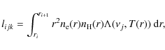
First, the wind structure from hydrodynamical simulations is used to
calculate the X-ray emissivity as a function of radius and frequency.
We divide the wind model into 29 equally spaced radial bins and
calculate the total wind X-ray emission in each radial bin at the
timestep k as an integral
|
(1) |
where the radius ri denotes the radial boundary of the ith bin,

where
|
(3) |
To provide a simpler description of the X-ray emission, we fit the values of
![]() by (see Fig. 1)
by (see Fig. 1)
where
Note that
where
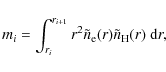
3.2 Temperature distribution fitting
Instead of fitting the X-ray emissivity from simulations directly,
it is also possible to fit the temperature distribution of X-ray
emitting gas. This approach does not explicitly depend on a particular
functional form of the X-ray emissivity
![]() ,
but is also not completely independent of it, as the distribution
of temperatures in the numerical simulations depends on the adopted
form of the cooling function.
,
but is also not completely independent of it, as the distribution
of temperatures in the numerical simulations depends on the adopted
form of the cooling function.
As the amount of emitted X-rays per unit volume of gas depends on the square of the density n2, it is not realistic to fit just the distribution of temperatures. To account for the correlation of the distribution of n2 with temperature, we evaluate for each timestep k the quantity similar to the differential emission measure (e.g., Dzifcáková et al. 2008)
|
(7) |
where
|
(8) |
where
![\begin{figure}
\par\includegraphics[width=8.5cm,clip]{12642fg3.eps}\hspace*{5mm}
\includegraphics[width=8.5cm,clip]{12642fg4.eps}
\end{figure}](/articles/aa/full_html/2009/47/aa12642-09/img55.png)
|
Figure 2:
Left: the temperature distribution of X-ray emitting gas expressed as
|
| Open with DEXTER | |
To provide a simpler description of
![]() we approximate it by a polynomial fit as
we approximate it by a polynomial fit as
where
Note that
where we set
We checked that both approximations of X-ray emission from hydrodynamical simulations (Eqs. (6) or (11)) and models based on exact data give similar results.
3.3 Scaling of X-ray emissivity with stellar parameters
The X-ray emission in the hydrodynamical wind simulations of Feldmeier et al. (1997a) was obtained for a mass-loss rate
![]()
![]()
![]() ,
radius
,
radius
![]() ,
and terminal velocity
,
and terminal velocity
![]() corresponding to a hydrodynamical wind model of
corresponding to a hydrodynamical wind model of ![]() Ori A.
Most of the X-rays used in these simulations originate
due to the collisions of fast clouds with dense shell fragments, where
the cloud formation is triggered by a turbulent photospheric seed
perturbation. Consequently, it is not clear whether the derived
analytical approximations are realistic also for other stars.
To account for the difference between the X-ray emission in
individual star wind models and
Ori A.
Most of the X-rays used in these simulations originate
due to the collisions of fast clouds with dense shell fragments, where
the cloud formation is triggered by a turbulent photospheric seed
perturbation. Consequently, it is not clear whether the derived
analytical approximations are realistic also for other stars.
To account for the difference between the X-ray emission in
individual star wind models and ![]() Ori A model of Feldmeier et al. (1997a), we introduced a scaling factor f* in Eqs. (6), (11).
Ori A model of Feldmeier et al. (1997a), we introduced a scaling factor f* in Eqs. (6), (11).
The X-ray emissivity is given by the rate of energy dissipation by
shocks. Neglecting possible dependencies on velocity and base
perturbations, we expect the rate of energy dissipation to be
proportional to the wind density. However, this is not what we would
get from the scaling
![]() in Eqs. (6), (11) with neglected dependence on the individual
wind parameters, i.e. with f*=1.
The reason is that we did not take into account that the fraction of
X-ray emitting material may not be the same for all stars. In the winds
with similar abundances, the radiative cooling is more efficient in
stars with denser winds than in stars with low-density winds. In the
winds with low density, a larger fraction of the wind gas may be
involved in radiating away the shock thermal energy.
in Eqs. (6), (11) with neglected dependence on the individual
wind parameters, i.e. with f*=1.
The reason is that we did not take into account that the fraction of
X-ray emitting material may not be the same for all stars. In the winds
with similar abundances, the radiative cooling is more efficient in
stars with denser winds than in stars with low-density winds. In the
winds with low density, a larger fraction of the wind gas may be
involved in radiating away the shock thermal energy.
Based on these arguments, we could introduce the scaling of f* with the density ![]() at a given point in the wind as
at a given point in the wind as
![]() .
However, this is not the most convenient scaling, as it would
introduce additional dependence of f* on the radius, which is already accounted for in Eqs. (6), (11). Consequently, for each star the value of f* should be fixed. Taking into account that
.
However, this is not the most convenient scaling, as it would
introduce additional dependence of f* on the radius, which is already accounted for in Eqs. (6), (11). Consequently, for each star the value of f* should be fixed. Taking into account that
![]() ,
we introduce a representative wind density
,
we introduce a representative wind density
![]() and in our calculations use
and in our calculations use
where R*,
4 Comparison with the ``filling factor'' approach
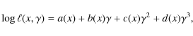
![\begin{figure}
\par\mbox{\includegraphics[width=8.8cm]{12642fg5.eps}\includegraphics[width=8.8cm]{12642fg6.eps} }\end{figure}](/articles/aa/full_html/2009/47/aa12642-09/img78.png)
|
Figure 3:
Left: the frequency distribution of X-rays derived using the ``filling factor'' approach expressed in terms of
|
| Open with DEXTER | |
It is informative to compare the X-ray spectrum and the temperature distribution function derived from hydrodynamic simulations in the previous section with those derived using simple ``filling factor'' approach. The filling factor determines the amount of X-ray emitting material.
We calculated the wind model of ![]() Ori A with X-ray emission included after the ``filling factor'' approach of Krticka & Kubát (2009)
and derived the resulting frequency distribution of emitted X-rays and
the temperature distribution of X-ray emitting gas (see Fig. 3).
The adopted model assumes that the temperature of the X-ray emitting
gas is given by the Rankine-Hugoniot condition with the velocity
difference related to the wind speed. Consequently, the temperature of
X-ray emitting gas in Fig. 3 increases with radius and X-rays are harder in outer wind parts.
Ori A with X-ray emission included after the ``filling factor'' approach of Krticka & Kubát (2009)
and derived the resulting frequency distribution of emitted X-rays and
the temperature distribution of X-ray emitting gas (see Fig. 3).
The adopted model assumes that the temperature of the X-ray emitting
gas is given by the Rankine-Hugoniot condition with the velocity
difference related to the wind speed. Consequently, the temperature of
X-ray emitting gas in Fig. 3 increases with radius and X-rays are harder in outer wind parts.
This is different from the results of hydrodynamical simulations. In the simulations the highest temperatures of X-ray emitting gas are achieved close to the star (see Fig. 2). As a result, the most energetic X-rays are emitted close to the star (see Fig. 1). Such a temperature distribution is supported by observations, as was inferred by Waldron & Cassinelli (2007) from their extensive analysis of high-resolution X-ray spectra of O stars. Consequently, two important features of the X-ray emission emerge from our simulations (and from observations): the decrease of the temperature of X-ray emitting gas with radius in the outer wind, and the multitemperature distribution of X-ray emitting gas at a given point.
5 Non-LTE models
5.1 Model assumptions
As an application of derived analytical formulae, we include X-ray emission parameterised by Eqs. (11) and (12) into our stationary, spherically symmetric non-LTE wind model (see Krticka & Kubát 2009, for a detailed description). The X-ray emission is included in the radiative transfer equation of our models. In the following we discuss just the temperature fitting approach as it seems to be more straightforward. The hydrogen and free electron densities in the X-ray source term are taken from the non-LTE models.
The excitation and ionization state of the considered elements is calculated from statistical equilibrium (non-LTE) equations. We use atomic data from the Opacity Project and the Iron Project (Seaton 1987; Fernley et al. 1987; Luo & Pradhan 1989; Sawey & Berrington 1992; Seaton et al. 1992; Butler et al. 1993; Nahar & Pradhan 1993; Hummer et al. 1993; Bautista 1996; Nahar & Pradhan 1996; Zhang 1996; Bautista & Pradhan 1997; Zhang & Pradhan 1997; Chen & Pradhan 1999). A significant part of the ionic models was taken from the TLUSTY code (Lanz & Hubeny 2007,2003). For phosphorus we employed data described by Pauldrach et al. (2001). Auger photoionization cross sections from individual inner-shells were taken from Verner & Yakovlev (1995, see also Verner et al. 1993#, and Auger yields were taken from Kaastra & Mewe (1993). We use Asplund et al. (2005) solar abundance determinations in the code.
The radiative transfer equation is split in two parts, i.e., the continuum and line radiative transfer. The radiative transfer in the continuum is solved using the Feautrier method in spherical coordinates (Mihalas & Hummer 1974; or Kubát 1993) with inclusion of all free-free and bound-free transitions of the model ions. The radiative transfer in lines is solved in the Sobolev approximation (e.g., Castor 1974) neglecting continuum opacity and line overlaps.
The radiative force is calculated in the Sobolev approximation (see Castor 1974). The corresponding line data were extracted in 2002 from the VALD database (Piskunov et al. 1995; Kupka et al. 1999). The radiative cooling and heating terms are calculated using the electron thermal balance method (Kubát et al. 1999). For the calculation of these terms we use occupation numbers derived from the statistical equilibrium equations. Finally, the continuity equation, equation of motion, and energy equation are solved iteratively to obtain the wind density, velocity, and temperature structure.
The shortest wavelength considered in the models is 4.1 Å and the longest X-ray wavelength is defined as 100 Å.
Table 1: Stellar parameters of studied O stars.
5.2 Test stars
The purpose of our study is to investigate the trends in the X-ray emission known for all OB stars, rather than to study X-ray properties of individual objects. Therefore, we compiled a list of O stars that includes the objects of various luminosity classes, masses, and binarity status. By doing this, our list may be considered as representative of a diverse population of O stars found in real star clusters. This allows us to compare the trend in X-ray luminosity of our synthetic O star population with the real clusters recently observed by Sana et al. (2006) and Antokhin et al. (2008).
To address the ``weak wind problem'' (Bouret et al. 2003; Martins et al. 2005), we also included stars that should be subject to it, i.e., their observed wind lines are much weaker than expected (the bottom four stars below the horizontal line in Table 1).
The stellar parameters (see Table 1) are taken from Lamers et al. (1995), Repolust et al. (2004), Markova et al. (2004), and Martins et al. (2005). Note that the parameters derived by Repolust et al. (2004), Markova et al. (2004), and Martins et al. (2005) were obtained using blanketed model atmospheres, i.e., they should be more reliable than the older ones. Stellar masses were obtained using evolutionary tracks (Schaller et al. 1992). The mass-loss rates in Table 1 were theoretically predicted using our models discussed in Sect. 5.1.
6 Non-LTE models with X-ray emission from simulations
The inclusion of X-ray emission does not significantly modify the ionization fractions close to the star below the critical point radius where the mass-loss rate is fixed. Consequently, X-rays do not significantly modify the wind mass-loss rate, but may modify the wind terminal velocity by a few percent (Krticka & Kubát 2009).
6.1 X-ray luminosity
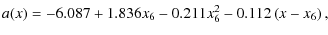
![\begin{figure}
\par\includegraphics[width=8cm,clip]{12642fg7.eps}
\end{figure}](/articles/aa/full_html/2009/47/aa12642-09/img107.png)
|
Figure 4: The dependence of the total X-ray luminosity on the bolometric luminosity calculated using non-LTE models with X-ray emissivity after Eqs. (11) and (12) (filled and empty circles) for individual stars. This is compared with the mean observational relations (corrected for the interstellar absorption) derived by Antokhin et al. (2008) and Sana et al. (2006, with uncertainty). Empty circles denote values for stars showing the ``weak wind problem''. |
| Open with DEXTER | |
A comparison of the predicted X-ray luminosities for individual stars and the mean observational trends is given in Fig. 4. The predicted X-ray luminosities for stars with optically thick winds (
![]() )
are on average lower roughly by a factor of three than the observed ones. This corresponds to the results of Feldmeier et al. (1997a).
)
are on average lower roughly by a factor of three than the observed ones. This corresponds to the results of Feldmeier et al. (1997a).
The derived slope of the
![]() relation for stars with optically thick winds,
relation for stars with optically thick winds,
![]() ,
is in better agreement with observations. The cause of the decrease of the slope (compared
to results obtained for a fixed filling factor as a free parameter, Krticka & Kubát 2009) can
be most easily understood from Fig. 1, which shows that
,
is in better agreement with observations. The cause of the decrease of the slope (compared
to results obtained for a fixed filling factor as a free parameter, Krticka & Kubát 2009) can
be most easily understood from Fig. 1, which shows that
![]() decreases with x (i.e., with radius). Consequently, the filling factor also decreases with radius, supporting the explanation of Owocki & Cohen (1999). Also the dependence of f* on the stellar parameters contributes to the decrease of the slope of the
decreases with x (i.e., with radius). Consequently, the filling factor also decreases with radius, supporting the explanation of Owocki & Cohen (1999). Also the dependence of f* on the stellar parameters contributes to the decrease of the slope of the
![]() relation, but the contribution of this parameter is sensitive to the stellar sample considered.
relation, but the contribution of this parameter is sensitive to the stellar sample considered.
For stars with optically thin wind (
![]() ), even the improved inclusion of X-ray emission is not capable of explaining the observed slope of the
), even the improved inclusion of X-ray emission is not capable of explaining the observed slope of the
![]() relation. As indicated
above, the dependence of the predicted X-ray luminosity of these stars on stellar luminosity
is steeper than for stars with high luminosity. However, this is not supported by observations. The
relation. As indicated
above, the dependence of the predicted X-ray luminosity of these stars on stellar luminosity
is steeper than for stars with high luminosity. However, this is not supported by observations. The
![]() relation of low luminosity stars is either the same as that of high luminosity stars,
or, for B stars, the slope is even less steep (Sana et al. 2006).
The reason for this discrepancy between observation and theory is
unclear. Note that for these stars the shock cooling length could be
comparable with the hydrodynamical scale (Krticka & Kubát 2009; Cohen et al. 2008).
The fact that a substantial fraction of the wind is too hot to give a
significant signature in the ultraviolet spectrum of the star could be
an explanation for the weak-wind problem (Krticka & Kubát 2009).
relation of low luminosity stars is either the same as that of high luminosity stars,
or, for B stars, the slope is even less steep (Sana et al. 2006).
The reason for this discrepancy between observation and theory is
unclear. Note that for these stars the shock cooling length could be
comparable with the hydrodynamical scale (Krticka & Kubát 2009; Cohen et al. 2008).
The fact that a substantial fraction of the wind is too hot to give a
significant signature in the ultraviolet spectrum of the star could be
an explanation for the weak-wind problem (Krticka & Kubát 2009).
6.2 The energy distribution of X-rays
![\begin{figure}
\par\includegraphics[width=7.5cm,clip]{12642fg8.eps}
\end{figure}](/articles/aa/full_html/2009/47/aa12642-09/img112.png)
|
Figure 5: Comparison between the predicted ratio of X-ray luminosities in the medium and soft energy bands for individual stars and the mean trend derived from observations. Main sequence stars are denoted with empty symbols, giants and supergiants with filled symbols. |
| Open with DEXTER | |
![\begin{figure}
\par\includegraphics[width=8cm,clip]{12642fg9.eps}\hspace*{0.8cm}
\includegraphics[width=8cm,clip]{12642fgA.eps}
\end{figure}](/articles/aa/full_html/2009/47/aa12642-09/img114.png)
|
Figure 6:
Ionization fractions as a function of the effective temperature for individual stars from our sample (only stars with
|
| Open with DEXTER | |
Sana et al. (2006) and Antokhin et al. (2008) divide the X-rays into three energy bands, soft (0.5-1.0 keV), medium (1.0-2.5 keV), and hard (
2.5-10.0 keV). The observations show that the slope of the
![]() relation
is roughly the same in the soft and medium band as in the total X-ray
emission, whereas the observations in the hard band show a large
dispersion.
relation
is roughly the same in the soft and medium band as in the total X-ray
emission, whereas the observations in the hard band show a large
dispersion.
Our calculations show a somewhat different result, as can be seen from Fig. 5, where we plot the ratio of the X-ray luminosities in the medium (![]() )
and soft (
)
and soft (![]() )
energy bands. The predicted slope of the
)
energy bands. The predicted slope of the
![]() relation in the medium band is steeper than that in the soft band, consequently the ratio of
relation in the medium band is steeper than that in the soft band, consequently the ratio of
![]() increases with luminosity. The reason
for this behaviour is the inverse proportionality of X-ray opacity and energy (e.g. Oskinova et al. 2006; Krticka & Kubát 2009).
For stars with low luminosities, the wind density is low, and most of
the emitted X-rays will be emergent. On the other hand, for stars with
high luminosities, density and opacity values become large, more flux
is absorbed in the soft than in the medium energy band, consequently
the emergent X-rays become harder. This also explains why the predicted
hardness of X-rays is greater for giants and supergiants than for main
sequence stars (see Fig. 5).
Finally, although from our models it follows that the predicted
dispersion of X-ray luminosities is indeed higher in the hard band than
in the medium and soft energy bands, there is still a clearly
discernible
increases with luminosity. The reason
for this behaviour is the inverse proportionality of X-ray opacity and energy (e.g. Oskinova et al. 2006; Krticka & Kubát 2009).
For stars with low luminosities, the wind density is low, and most of
the emitted X-rays will be emergent. On the other hand, for stars with
high luminosities, density and opacity values become large, more flux
is absorbed in the soft than in the medium energy band, consequently
the emergent X-rays become harder. This also explains why the predicted
hardness of X-rays is greater for giants and supergiants than for main
sequence stars (see Fig. 5).
Finally, although from our models it follows that the predicted
dispersion of X-ray luminosities is indeed higher in the hard band than
in the medium and soft energy bands, there is still a clearly
discernible
![]() relation even in the hard band.
relation even in the hard band.
6.3 Ionization fractions
The presence of X-rays may also influence the ionization fractions of highly ionised ions. We plot in Fig. 6 the predicted ionization fractions in comparison with those derived from observation as a function of effective stellar temperature. Note that here we use the ionization fractions derived for LMC stars (Massa et al. 2003), because their observational sample includes a large number of ionization stages, the fractions of which are given as a function of velocity, and the wind parameters of LMC stars are not significantly different from Galactic ones. Since several parameters except the effective temperature (e.g., the wind density) may influence the ionization fractions, the graphs in Fig. 6 are not monotonic.
In Fig. 6 we also plot the results of Krticka & Kubát (2009), which were obtained using a simpler inclusion of X-rays assuming a constant filling factor (see also Sect. 4). Still, the emergent X-ray luminosities from these models roughly correspond to the observed ones. Rather surprisingly, although the non-LTE models calculated with X-ray emission from hydrodynamical wind simulations give a too low emergent X-ray luminosity, the ionization structure of these models corresponds in general much better to the trends derived from observations.
This better agreement between theoretical and observational ionization fractions may be due to an overall lower X-ray emissivity. To test this, we calculated models with a simplified treatment of X-ray emission after Krticka & Kubát (2009), but assuming the same X-ray luminosity as that predicted by hydrodynamical simulations. Our results show that even in this case the use of X-ray emissivity based on hydrodynamical simulation gives better agreement with observations. We conclude that the hydrodynamical simulations give a more realistic dependence of the X-ray emissivity on frequency.
7 Discussion
The remaining discrepancy between theory and observation may originate in our neglect of macroclumping (sometimes also termed porosity). The macroclumping may cause a lower opacity in the X-ray domain, which leads to a higher predicted X-ray luminosity. From Fig. 17 in Oskinova et al. (2004), it follows that an increase of X-ray luminosity by a factor of 3 would be easily achievable. Accounting for macroclumping reduces the wavelength dependence of opacity. In its limit (when clumps are fully opaque), the opacity becomes grey (Oskinova et al. 2004).
Wind inhomogeneities should also affect the ionization fractions. Optically thin inhomogeneities (often referred to as ``microclumping'') lead generally to lower ionization stages (de Koter et al. 2008; Krticka et al. 2008), hence clumping with increased X-ray emissivity could be another way to explain the X-ray luminosities and ionization fractions derived from observation.
Our hydrodynamical wind simulations assume 1D spherical symmetry, thus all wind structures correspond to full spherical shells. Therefore, we have at present a very limited knowledge of real wind clumping.
To be consistent with the hydrodynamical simulations, we use the Raymond-Smith X-ray spectral code (Raymond & Smith 1977; Raymond 1988), although it would be possible to use codes based on up-to-date atomic data. Our test using the APEC subroutine available in XSPEC (Smith et al. 2001; Arnaud 1996) showed that there is a relatively good agreement between the fits using this and the Raymond-Smith code Eq. (5).
8 Summary
We provide analytical approximations of the X-ray emission predicted by hydrodynamical simulations of hot star winds by Feldmeier et al. (1997a). The X-ray emission derived from the hydrodynamical simulations has two distinctive aspects. First, the temperature of X-ray emitting gas decreases with radius in the outer wind. Second, the temperature of the X-ray emitting gas is described by a distribution function, which is more realistic than assuming just one temperature at a given point.
We include these approximations in non-LTE models (Krticka & Kubát 2009)
and for selected stars compare the resulting X-ray luminosities, energy
distribution of emergent X-rays, and ionization structure with
observational results. We conclude that although the predicted X-ray
luminosity is slightly underestimated, the resulting ionization
structure is in relatively good agreement with observations. Earlier
papers debated whether the theory of line-driven winds can explain the
observed
![]() relation. Our results reproduce this scaling.
relation. Our results reproduce this scaling.
We thank the referee for his/her comments that helped to improve the manuscript. This work was supported by grant GA CR 205/08/0003. L.M.O. acknowledges the support of DLR grant 50 OR 0804.
References
- Antokhin, I. I., Rauw, G., Vreux, J.-M., van der Hucht, K. A., & Brown, J. C. 2008, A&A, 477, 593 [NASA ADS] [EDP Sciences] [CrossRef]
- Arnaud, K. A. 1996, Astronomical Data Analysis Software and Systems V, ed. G. Jacoby, & J. Barnes (San Francisco: ASP), 17
- Asplund, M., Grevesse, N., & Sauval, A. J. 2005, Cosmic Abundances as Records of Stellar Evolution and Nucleosynthesis, ed. T. G. Barnes III, & F. N. Bash (San Francisco: ASP), ASP Conf. Ser., 336, 25
- Babel, J., & Montmerle, T. 1997, A&A, 323, 121 [NASA ADS]
- Benaglia, P., Vink, J. S., Martí, J., et al. 2007, A&A, 467, 1265 [NASA ADS] [EDP Sciences] [CrossRef]
- Bautista, M. A. 1996, A&AS, 119, 105 [NASA ADS] [EDP Sciences] [CrossRef]
- Bautista, M. A., & Pradhan, A. K. 1997, A&AS, 126, 365 [NASA ADS] [EDP Sciences] [CrossRef]
- Berghöfer, T. W., Schmitt, J. H. M. M., Danner, R., & Cassinelli, J. P. 1997, A&A, 322, 167 [NASA ADS]
- Bianchi, L., Bohlin, R., & Massey, P. 2004, ApJ, 601, 228 [NASA ADS] [CrossRef]
- Bouret, J.-C., Lanz, T., Hillier, D. J., et al. 2003, ApJ, 595, 1182 [NASA ADS] [CrossRef]
- Burgers, J. M. 1974, The Nonlinear Diffusion Equation (Dordrecht: Reidel)
- Butler, K., Mendoza, C., & Zeippen, C. J. 1993, J. Phys. B., 26, 4409 [NASA ADS] [CrossRef]
- Castor, J. I. 1974, MNRAS, 169, 279 [NASA ADS]
- Chen, G. X., & Pradhan, A. K. 1999, A&AS, 136, 395 [NASA ADS] [EDP Sciences] [CrossRef]
- Cooke, B. A., Fabian, A. C., & Pringle, J. E. 1978, Nature, 273, 645 [NASA ADS] [CrossRef]
- Chlebowski, T., Harnden, F. R., & Sciortino, S. 1989, ApJ, 341, 427 [NASA ADS] [CrossRef]
- Cohen, D. H., Kuhn, M. A., Gagné, M., Jensen, E. L. N., & Miller, N. A. 2008, MNRAS, 386, 1855 [NASA ADS] [CrossRef]
- de Koter, A., Vink, J. S., & Muijres, L. 2008, in Clumping in Hot Star Winds, ed. W.-R. Hamann, A. Feldmeier, & L. Oskinova, 47
- Dzifcáková, E., Kulinová, A., Chifor, C., et al. 2008, A&A, 488, 311 [NASA ADS] [EDP Sciences] [CrossRef]
- Feldmeier, A. 1995, A&A, 299, 523 [NASA ADS]
- Feldmeier, A., Puls, J., & Pauldrach, A. W. A. 1997a, A&A, 322, 878 [NASA ADS]
- Feldmeier, A., Kudritzki, R.-P., Palsa, R., Pauldrach, A. W. A., & Puls, J. 1997b, A&A, 320, 899 [NASA ADS]
- Feldmeier, A., Oskinova, L., & Hamann, W.-R. 2003, A&A, 403, 217 [NASA ADS] [EDP Sciences] [CrossRef]
- Fernley, J. A., Taylor, K. T., & Seaton, M. J. 1987, J. Phys. B, 20, 6457 [NASA ADS] [CrossRef]
- Hedstrom, G. W. 1979, J. Comp. Phys., 30, 222 [NASA ADS] [CrossRef]
- Hillier, D. J., Kudritzki, R. P., Pauldrach, A., et al. 1993, A&A, 276
- Hummer, D. G., Berrington, K. A., Eissner, W., et al. 1993, A&A, 279, 298 [NASA ADS]
- Kaastra, J. S., & Mewe, R. 1993, A&AS, 97, 443 [NASA ADS]
- Krticka, J. 2006, MNRAS, 367, 1282 [NASA ADS] [CrossRef]
- Krticka, J., & Kubát, J. 2009, MNRAS, 394, 2065 [NASA ADS] [CrossRef]
- Krticka, J., Puls, J., & Kubát, J. 2008, in Clumping in Hot Star Winds, ed. W.-R. Hamann, A. Feldmeier, & L. Oskinova, 111
- Kubát, J. 1993, Ph.D. Thesis, Astronomický ústav AV CR, Ondrejov
- Kubát, J., Puls, J., & Pauldrach, A. W. A. 1999, A&A, 341, 587 [NASA ADS]
- Kudritzki, R. P., & Puls, J. 2000, ARA&A, 38, 613 [NASA ADS] [CrossRef]
- Kupka, F., Piskunov, N. E., Ryabchikova, T. A., Stempels, H. C., & Weiss, W. W. 1999, A&AS, 138, 119 [NASA ADS] [EDP Sciences] [CrossRef]
- Lamb, H. 1945, Hydrodynamics (New York: Dover)
- Lamers, H. J. G. L. M., Snow, T. P., & Lindholm, D. M. 1995, ApJ, 455, 269 [NASA ADS] [CrossRef]
- Langer, S. H., Chanmugam, G., & Shaviv, G. 1981, ApJ, 245, L23 [NASA ADS] [CrossRef]
- Lanz, T., & Hubeny, I. 2003, ApJS, 146, 417 [NASA ADS] [CrossRef]
- Lanz, T., & Hubeny, I. 2007, ApJS, 169, 83 [NASA ADS] [CrossRef]
- Lucy, L. B. 1984, ApJ, 284, 351 [NASA ADS] [CrossRef]
- Lucy, L. B., & Solomon, P. M. 1970, ApJ, 159, 879 [NASA ADS] [CrossRef]
- Luo, D., & Pradhan, A. K. 1989, J. Phys. B, 22, 3377 [NASA ADS] [CrossRef]
- MacGregor, K. B., Hartmann, L., & Raymond, J. C. 1979, ApJ, 231, 514 [NASA ADS] [CrossRef]
- Markova, N., Puls, J., Repolust, T., & Markov, H. 2004, A&A, 413, 693 [NASA ADS] [EDP Sciences] [CrossRef]
- Martins, F., Schaerer, D., Hillier, D. J., et al. 2005, A&A, 441, 735 [NASA ADS] [EDP Sciences] [CrossRef]
- Mihalas, D., & Hummer, D. G. 1974, ApJS, 28, 343 [NASA ADS] [CrossRef]
- Massa, D., Fullerton, A. W., Sonneborn, G., & Hutchings, J. B. 2003, ApJ, 586, 996 [NASA ADS] [CrossRef]
- MacFarlane, J. J., Cohen, D. H., & Wang, P. 1994, ApJ, 437, 351 [NASA ADS] [CrossRef]
- Nahar, S. N., & Pradhan, A. K. 1993, J. Phys. B, 26, 1109 [NASA ADS] [CrossRef]
- Nahar, S. N., & Pradhan, A. K. 1996, A&AS, 119, 509 [NASA ADS] [EDP Sciences] [CrossRef]
- Oskinova, L. M., Feldmeier, A., & Hamann, W.-R. 2004, A&A, 422, 675 [NASA ADS] [EDP Sciences] [CrossRef]
- Oskinova, L. M., Feldmeier, A., & Hamann, W.-R. 2006, MNRAS, 372, 313 [NASA ADS] [CrossRef]
- Owocki, S. P. 1991, in Stellar Atmospheres: Beyond Classical Models, ed. L. Crivellari, I. Hubeny, & D. G. Hummer (Dordrecht: Kluwer), 235
- Owocki, S. P., & Cohen, D. H. 1999, ApJ, 520, 833 [NASA ADS] [CrossRef]
- Owocki, S. P., & Puls, J. 1996, ApJ, 462, 894 [NASA ADS] [CrossRef]
- Owocki, S. P., & Rybicki, G. B. 1985, ApJ, 299, 265 [NASA ADS] [CrossRef]
- Owocki, S. P., Castor, J. I., & Rybicki, G. B. 1988, ApJ, 335, 914 [NASA ADS] [CrossRef]
- Owocki, S. P., Gayley, K. G., & Shaviv, N. J. 2004, ApJ, 616, 525 [NASA ADS] [CrossRef]
- Pauldrach, A., Puls, J., & Kudritzki, R. P. 1986, A&A, 164, 86 [NASA ADS]
- Pauldrach, A. W. A., Hoffmann, T. L., & Lennon, M. 2001, A&A, 375, 161 [NASA ADS] [EDP Sciences] [CrossRef]
- Piskunov, N. E., Kupka, F., Ryabchikova, T. A., Weiss, W. W., & Jeffery, C. S. 1995, A&AS, 112, 525 [NASA ADS]
- Pittard, J. M. 2009, MNRAS, 396, 1743 [NASA ADS] [CrossRef]
- Poe, C. H., Owocki, S. P., & Castor, J. I. 1990, ApJ, 358, 199 [NASA ADS] [CrossRef]
- Prilutskii, O. F., & Usov, V. V. 1976, AZh, 53, 6 [NASA ADS]
- Puls, J., Markova, N., Scuderi, S., et al. 2006, A&A, 454, 625 [NASA ADS] [EDP Sciences] [CrossRef]
- Puls, J., Markova, N., & Scuderi, S. 2008a, Mass Loss from Stars and the Evolution of Stellar Clusters, ed. A. de Koter, L. Smith, & R. Waters (San Francisco: ASP), 101
- Puls, J., Vink, J. S., & Najarro, F. 2008b, A&ARv, 16, 209 [NASA ADS]
- Raymond, J. C. 1988, in Hot Thin Plasmas in Astrophysics, NATO ASI Series C, ed. R. Pallavicini, 249, 3
- Raymond, J. C., & Smith, B. W. 1977, ApJS, 35, 419 [NASA ADS] [CrossRef]
- Repolust, T., Puls, J., & Herrero, A. 2004, A&A, 415, 349 [NASA ADS] [EDP Sciences] [CrossRef]
- Risken, H. 1996, The Fokker-Planck Equation (Heidelberg: Springer)
- Sana, H., Rauw, G., Nazé, Y., Gosset, E., & Vreux, J.-M. 2006, MNRAS, 372, 661 [NASA ADS] [CrossRef]
- Sawey, P. M. J., & Berrington, K. A. 1992, J. Phys. B, 25, 1451 [NASA ADS] [CrossRef]
- Schaller, G., Schaerer, D., Meynet, G., & Maeder, A. 1992, A&AS, 96, 269 [NASA ADS]
- Seaton, M. J. 1987, J. Phys. B, 20, 6363 [NASA ADS] [CrossRef]
- Seaton, M. J., Zeippen, C. J., Tully, J. A., et al. 1992, Rev. Mex. Astron. Astrofis., 23, 19 [NASA ADS]
- Smith, R. K., Brickhouse, N. S., Liedahl, D. A., & Raymond, J. C. 2001, ApJ, 556, 91 [NASA ADS] [CrossRef]
- Thompson, K. W. 1987, J. Comp. Phys., 68, 1 [NASA ADS] [CrossRef]
- Thompson, K. W. 1990, J. Comp. Phys., 89, 439 [NASA ADS] [CrossRef]
- ud-Doula, A., & Owocki, S. P. 2002, ApJ, 576, 413 [NASA ADS] [CrossRef]
- van Leer, B. 1977, J. Comp. Phys., 23, 276 [NASA ADS] [CrossRef]
- Verner, D. A., & Yakovlev, D. G. 1995, A&AS, 109, 125 [NASA ADS]
- Verner, D. A., Yakovlev, D. G., Band, I. M., & Trzhaskovskaya, M. B. 1993, Atomic Data and Nuclear Data Tables, 55, 233 [NASA ADS] [CrossRef]
- Vink, J. S., de Koter, A., & Lamers, H. J. G. L. M. 2000, A&A, 362, 295 [NASA ADS]
- Vink, J. S., de Koter, A., & Lamers, H. J. G. L. M. 2001, A&A, 369, 574 [NASA ADS] [EDP Sciences] [CrossRef]
- Waldron, W. L., & Cassinelli, J. P. 2007, ApJ, 668, 456 [NASA ADS] [CrossRef]
- Zhang, H. L. 1996, A&AS, 119, 523 [NASA ADS] [EDP Sciences] [CrossRef]
- Zhang, H. L., & Pradhan, A. K. 1997, A&AS, 126, 373 [NASA ADS] [EDP Sciences] [CrossRef]
Footnotes
- ... O stars
![[*]](/icons/foot_motif.png)
- Note that the situation may be different in late O and
B supergiants, for which the value
 might be a more appropriate one (Benaglia
et al. 2007).
might be a more appropriate one (Benaglia
et al. 2007).
All Tables
Table 1: Stellar parameters of studied O stars.
All Figures
|
|
Figure 1:
Left: the frequency distribution of X-rays expressed in terms of
|
| Open with DEXTER | |
| In the text | |
|
|
Figure 2:
Left: the temperature distribution of X-ray emitting gas expressed as
|
| Open with DEXTER | |
| In the text | |
|
|
Figure 3:
Left: the frequency distribution of X-rays derived using the ``filling factor'' approach expressed in terms of
|
| Open with DEXTER | |
| In the text | |
|
|
Figure 4: The dependence of the total X-ray luminosity on the bolometric luminosity calculated using non-LTE models with X-ray emissivity after Eqs. (11) and (12) (filled and empty circles) for individual stars. This is compared with the mean observational relations (corrected for the interstellar absorption) derived by Antokhin et al. (2008) and Sana et al. (2006, with uncertainty). Empty circles denote values for stars showing the ``weak wind problem''. |
| Open with DEXTER | |
| In the text | |
|
|
Figure 5: Comparison between the predicted ratio of X-ray luminosities in the medium and soft energy bands for individual stars and the mean trend derived from observations. Main sequence stars are denoted with empty symbols, giants and supergiants with filled symbols. |
| Open with DEXTER | |
| In the text | |
|
|
Figure 6:
Ionization fractions as a function of the effective temperature for individual stars from our sample (only stars with
|
| Open with DEXTER | |
| In the text | |
Copyright ESO 2009
Current usage metrics show cumulative count of Article Views (full-text article views including HTML views, PDF and ePub downloads, according to the available data) and Abstracts Views on Vision4Press platform.
Data correspond to usage on the plateform after 2015. The current usage metrics is available 48-96 hours after online publication and is updated daily on week days.
Initial download of the metrics may take a while.