| Issue |
A&A
Volume 507, Number 3, December I 2009
|
|
|---|---|---|
| Page(s) | 1785 - 1791 | |
| Section | Numerical methods and codes | |
| DOI | https://doi.org/10.1051/0004-6361/200912800 | |
| Published online | 24 September 2009 | |
A&A 507, 1785-1791 (2009)
Application of the coupled escape probability method to spherical clouds
Y. J. Yun - Y.-S. Park - S. H. Lee
Department of Physics and Astronomy, Seoul National University, Korea
Received 30 June 2009 / Accepted 21 August 2009
Abstract
Aims. We present applications of one of the novel radiative
transfer methods, called the coupled escape probability method, to
spherical clouds. It provides efficient tools for analyzing molecular
lines, but its implementation is limited to plane-parallel systems. For
more general uses, we extend its capability to spherical systems.
Methods. The spherical geometry means that the derivation of
mean intensity has to be conducted numerically, whereas it was done
more analytically in the original work. The new method was applied to
spherical clouds and cores with various conditions, and systems with
moderate systematic motion are tested in addition to static systems.
The case of molecular transitions with hyperfine overlap is also
investigated.
Results. While this method is more complicated than the original
method, it maintains the underlying simplicity and practicality. The
excitation conditions derived for the various conditions are compared
with those of the Monte Carlo methods, and the results are found
to be in good agreement with each other. The new method is more
efficient in computing time and number of iterations.
Key words: line: formation - radiative transfer - methods: numerical - ISM: molecules
1 Introduction
The progress of receiver technologies and the exploitation of high and dry sites have enabled radio observations at higher frequencies. Molecular transitions at such frequencies involve, in general, energy levels that are highly excited, thus reflecting the physical conditions of hot and/or dense regions in clouds or cores. Since populations will be distributed over a wide range of energy levels in this case, simply relying on the analysis of one or two transitions and/or on unrealistic assumptions will result in serious errors when deriving physical quantities. Thus, multi-transitional studies of molecular lines are crucial. This is the area where the non-LTE radiative transfer and excitation (RT hereafter) models can play an important role in calculating physical quantities such as column density and molecular abundances (van der Tak et al. 2007). The models also help for inferring velocity fields inside molecular clouds/cores through analysis of the line shape (e.g., Zhou et al. 1993; Lee et al. 2007).
Among these is the large velocity gradient (LVG) model, which has long
been used for its simplicity and robustness (Goldreich & Kwan 1974; van der Tak et al. 2007).
It actually solves the RT problem locally, based on the
assumption of the large systematic motion.
However, because this type of motion is very rare, the RT problem
cannot be solved locally.
Moreover, the model does not make use of information contained in the
line shape. The first rigorous non-LTE treatment of molecular
lines was made by Leung & Liszt (1976),
who solved the non-LTE RT model using the quasi-diffusion method.
This model can provide both line profiles and
excitation conditions, but cannot treat velocity fields properly except
for microturbulence. Although there have been several RT models
(van Zadelhoff et al. 2002, and references therein), the Monte Carlo method introduced by Bernes (1979)
may be the most popular one, even to this day. The model traces the
fate of real photons that are replaced by a much smaller number of
model photons that are spontaneously generated inside and come from
outside. Then, the mean radiation field and, accordingly, a number of
(de-)excitations are readily calculated and are fed into the
statistical equilibrium equation. The whole process is repeated via the
![]() -iteration
until convergence is obtained. Although noise is inherent in this
model, the velocity field can be taken into account properly, and
extension to a higher dimension is conceptually easy. This method has
been expanded into three-dimensional ones (Park & Hong 1995; Juvela 1997), improved to achieve better convergence with the accelerated
-iteration
until convergence is obtained. Although noise is inherent in this
model, the velocity field can be taken into account properly, and
extension to a higher dimension is conceptually easy. This method has
been expanded into three-dimensional ones (Park & Hong 1995; Juvela 1997), improved to achieve better convergence with the accelerated ![]() -iteration (Hogerheijde & van der Tak 2000), or both (Wada & Tomisaka
2005).
-iteration (Hogerheijde & van der Tak 2000), or both (Wada & Tomisaka
2005).
An interesting model of radiative transfer has been presented by Elitzur & Asensio Ramos (2006). By adopting the zone-based gridding in a plane-parallel system, they derive the equations of statistical equilibrium, which are fully consistent with the radiative transfer based on the assumption that all physical properties are constant within each zone. With this assumption, the equation of radiative transfer is solved explicitly and analytically, and can then be easily merged into the level population equations. These equations are linearized and globally solved. This method is called coupled escape probability (CEP) because the different zones are coupled through the net radiative bracket (Athay & Skumanich 1971), which resembles the standard escape probability expression.
A method based on the Gauss-Seidel algorithm presented by Trujillo Bueno & Fabiani Bendicho (1995) and extended by Asensio Ramos & Trujillo Bueno (2006) is also noteworthy. The basic concept of the algorithm is to update level populations and mean intensity, ![]() ,
whenever possible, in the course of sweeping grids from center to outer boundary. Daniel & Cernicharo (2008) introduce several assumptions into the
original Gauss-Seidel algorithm to reduce the computational time and applied the algorithm to the problem of N2H+ hyperfine lines in a spherical system.
,
whenever possible, in the course of sweeping grids from center to outer boundary. Daniel & Cernicharo (2008) introduce several assumptions into the
original Gauss-Seidel algorithm to reduce the computational time and applied the algorithm to the problem of N2H+ hyperfine lines in a spherical system.
We have tried to apply the CEP method to the spherical system. In contrast to the plane-parallel system, it will be difficult to make use of the analytical approach of the CEP method in the spherical system. More numerical works are necessary, but the CEP concept will be weakened. However, the RT equation is still readily and explicitly solved since each zone is constant in physical quantities. Consequently, the system could be linearized and solved efficiently with, for example, the Newton method. The CEP spherical model is applied to clouds both with and without a velocity field for the CO molecule. In addition, the excitation of molecules with hyperfine splitting, such as HCN, is investigated and compared with those from the Monte Carlo method. We describe the mathematical formulations in Sect. 2 and present results in Sect. 3. The discussion and conclusions are given in Sects. 4 and 5, respectively. Our final goal is to provide a handy tool for analyzing multi-transitional molecular lines with high fidelity and efficiency for spherical geometry.
2 Mathematical formulation
2.1 Radiative transfer
Here, we describe the mathematical formulation of radiative transfer in a spherical molecular cloud/core. For numerical work, the sphere is divided into many concentric shells, as usual. We assume that physical conditions are uniform within each zone. This assumption is not new and has been adopted in the Monte Carlo method (Bernes 1979), but it plays a crucial role in the CEP method. This assumption may be relaxed into a grid-based one, and a parabolic variation may be used for better realization of systems by sacrificing computation time and simplicity (Daniel & Cernicharo 2008).
Thus, specific intensity
![]() is readily calculated at a position in a zone along an arbitrary direction,
is readily calculated at a position in a zone along an arbitrary direction,
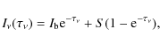
where S is source function and
where the
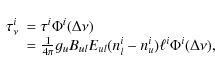
where
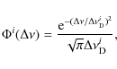
where
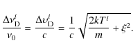
In Eq. (5),
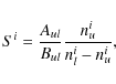
where Aul is the Einstein coefficient for the transition.
The boundary value,
![]() ,
depends on the ray direction, i.e., the sign of the angle cosine.
The sign of the angle cosine changes when the ray passes through the mth zone, which is the innermost zone passed by the ray (see Fig. 1). If the angle cosine at the outer boundary of the ith zone is
,
depends on the ray direction, i.e., the sign of the angle cosine.
The sign of the angle cosine changes when the ray passes through the mth zone, which is the innermost zone passed by the ray (see Fig. 1). If the angle cosine at the outer boundary of the ith zone is ![]() (inwardly moving rays), where
(inwardly moving rays), where ![]() is always positive, then
is always positive, then
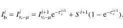
The
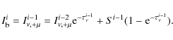
This equation is applied successively down to the mth zone, and after that the Eq. (7) should again be used. If, e.g., a (proto-)star resides at the center, the inner boundary conditions are set by
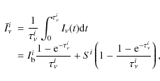
There may be various ways of numerically deriving the mean intensity of the ith zone,
averaged over both angles and frequencies to be used in the equation of
statistical equilibrium. We adopt the following equation by making use
of the averaged specific intensity of Eq. (2):
In the case of a finite slab, the double integration in Eq. (9) is performed and simply expressed in terms of escape probabilities (Elitzur & Asensio Ramos 2006). However, in the spherical system, the analytical integration is not possible, so the integration must be performed numerically. As a result, the concept of escape probability is not introduced explicitly for the spherical systems. For the integration over a solid angle in Eq. (9), one calculates
Another factor to consider is that the angle cosine, ![]() ,
of a ray is not constant along a ray path, even in the same zone. Thus, as we have done for
,
of a ray is not constant along a ray path, even in the same zone. Thus, as we have done for
![]() ,
we need to average the
angle cosine to obtain a representative value,
,
we need to average the
angle cosine to obtain a representative value,
![]() ,
for numerical integration. One way of deriving
,
for numerical integration. One way of deriving
![]() is to average the angle cosine over the path length of the ith zone as follows:
is to average the angle cosine over the path length of the ith zone as follows:
After completing some algebra, it is found that
where
The
Finally, we are able to write the mean intensity integrated over absorption profile of the ith zone as
![\begin{displaymath}%
\bar{J}^i=\frac{1}{2 N_{\rm ray} N_f}
\sum^{N_{\rm ray}}_{s...
...{i}_{\nu,+\mu_s}W^i_{+\bar{\mu}_s}\right]\Phi^i (\Delta\nu_f),
\end{displaymath}](/articles/aa/full_html/2009/45/aa12800-09/img55.png)
where
![\begin{figure}
\par\includegraphics[width=8.8cm,clip]{12800fg1.eps}
\end{figure}](/articles/aa/full_html/2009/45/aa12800-09/img63.png)
|
Figure 1: Geometric quantities of the model. |
| Open with DEXTER | |
2.2 Statistical equilibrium
One of the advantages of assuming that physical conditions are uniform in each zone is that one can explicitly see the dependencies of the mean intensity in a zone on level populations in other zones. This is possible since the mean specific intensity is analytically obtained, though it is within double summation. This enables us to linearize the rate equation and to solve it using the Newton method, after forming the Jacobian.
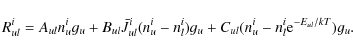
We denote the statistical weight of each level by gl, and the population per sublevel in the zone, i by nil. The steady-state rate equations for a molecule with L levels in the ith zone are
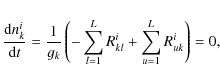
where
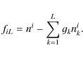
These are L-1 independent equations for the L unknown populations in each zone. We can make this system closed by using

which is the overall population in the zone, i for the multi-level system.
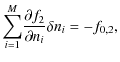
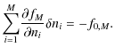
Equations (14) and (16) form a set of nonlinear algebraic equations. For the system with L levels and N zones, the M=NL equations are given as
where, for
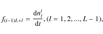
and for l=L,
Usually, Eq. (17) is solved using the


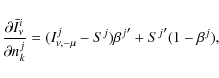
We first assume level populations, then calculate the Jacobian,
![\begin{displaymath}%
\frac{\partial\bar{I}^i_{\nu}}{\partial n^j_k}=\frac{\parti...
...ac{1-{\rm e}^{-\tau^i_{\nu}}}{\tau^i_{\nu}}\right)\right]\cdot
\end{displaymath}](/articles/aa/full_html/2009/45/aa12800-09/img79.png)
In light of Eqs. (7) and (8), both for
- i)
- j<i;
- ii)
- j=i;
- iii)
- j>i;

![\begin{displaymath}%
\frac{\partial \bar{I}^i_{\nu}}{\partial n^j_k}
=\beta^i \p...
...+1}E^t
\left[(I^j_{\nu,-\mu}-S^j) {E^j}'+{S^j}'(1-E^j)\right].
\end{displaymath}](/articles/aa/full_html/2009/45/aa12800-09/img82.png)
- i)
- j<i;
- ii)
- j=i;
- iii)
- j>i;
where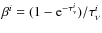 ,
and
,
and
 .
The derivatives on S,
.
The derivatives on S,
 ,
and
,
and  are straightforward, so will not be iterated here.
![$\displaystyle \beta^i \displaystyle{\prod^{i-1}_{t=j+1}E^t}
\left[(I^{j-1}_{\nu,+\mu}-S^j){E^j}'+{S^j}'(1-E^j)\right]$](/articles/aa/full_html/2009/45/aa12800-09/img84.png)
![$\displaystyle + ~\beta^i \displaystyle{\prod^{j-1}_{t=m}E^t}\displaystyle{\prod...
..._{t=m+1}E^t}
\left[(I^j_{\nu,-\mu}\!-\!S^j){E^j}'\!+\!{S^j}'(1\!-\!E^j)\right],$](/articles/aa/full_html/2009/45/aa12800-09/img85.png)
![$\displaystyle + ~\beta^j \displaystyle{\prod^{j-1}_{t=m}E^t}\displaystyle{\prod...
..._{t=m+1}E^t}
\left[(I^j_{\nu,-\mu}\!-\!S^j){E^j}'\!+\!{S^j}'(1\!-\!E^j)\right],$](/articles/aa/full_html/2009/45/aa12800-09/img87.png)
![\begin{displaymath}%
\frac{\partial \bar{I}^i_{\nu}}{\partial n^j_k}
=\beta^i \d...
...+1}E^t}
\left[(I^j_{\nu,-\mu}-S^j){E^j}'+{S^j}'(1-E^j)\right],
\end{displaymath}](/articles/aa/full_html/2009/45/aa12800-09/img88.png)
The grand Jacobian matrix consists of N ![]() N block matrices, and a block matrix is composed of L
N block matrices, and a block matrix is composed of L ![]() L elements. Diagonal blocks represent radiative and
collisional interactions among the energy levels in the same zones,
while nondiagonal blocks involve nonlocal radiative interactions
between different zones. The simpler the transition network, the
sparser the Jacobian. The Jacobian is formed in this way and the
nonlinear equations are solved using the Newton method.
L elements. Diagonal blocks represent radiative and
collisional interactions among the energy levels in the same zones,
while nondiagonal blocks involve nonlocal radiative interactions
between different zones. The simpler the transition network, the
sparser the Jacobian. The Jacobian is formed in this way and the
nonlinear equations are solved using the Newton method.
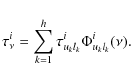
2.3 Overlap of hyperfine lines
For the overlapping lines, the source function is no longer independent of frequency. Assuming that there are h overlapping transitions, we denote the upper levels by
u1,u2,...,uh and the lower levels by
l1,l2,...,lh in the transitions. The source function of the ith zone is given by
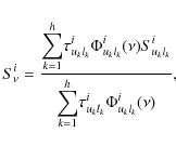
where Siuklk is the frequency-independent source function, which is the same as Eq. (6). The optical depth is also obtained using the summation of the line optical depths involved in the overlaps. They are given by
The intensity of the ith zone,
![\begin{figure}
\par\includegraphics[width=8.5cm,clip]{12800fg2.eps}
\end{figure}](/articles/aa/full_html/2009/45/aa12800-09/img98.png)
|
Figure 2: Excitation temperatures
of CO molecules against the normalized radial distance of static
clouds with the kinetic temperature of
|
| Open with DEXTER | |
![\begin{figure}
\par\includegraphics[width=8.5cm,clip]{12800fg3.eps}
\end{figure}](/articles/aa/full_html/2009/45/aa12800-09/img99.png)
|
Figure 3:
Excitation temperatures of CO molecules against the normalized
radial distance of a cloud under systematic motion with the kinetic
temperature of
|
| Open with DEXTER | |
3 Results
Our method is tested for a few cloud models in transitions both with and without line overlaps. Its results are compared with those from the Monte Carlo method.
3.1 Static molecular clouds
First, we test the method by applying it to the static clouds. The radius is
![]() ,
the kinetic temperature is
,
the kinetic temperature is
![]() ,
and the Doppler velocity width is set to
,
and the Doppler velocity width is set to
![]() .
Two density models are used for this calculation: the first one has a constant density of
.
Two density models are used for this calculation: the first one has a constant density of
![]() ,
and the second a density gradient of
,
and the second a density gradient of
![]() .
The relative abundance of CO to H2 is set to 10-5 for both cases. All models are calculated for L=10 lower levels of CO, and
we use N=20 zones of equal spacing. Collisional coefficients by Flower (2001) and Wernli et al. (2006) are adopted for CO molecules. Figure 2 shows the results from our method and from the Monte Carlo method as well. We used the accelerated
.
The relative abundance of CO to H2 is set to 10-5 for both cases. All models are calculated for L=10 lower levels of CO, and
we use N=20 zones of equal spacing. Collisional coefficients by Flower (2001) and Wernli et al. (2006) are adopted for CO molecules. Figure 2 shows the results from our method and from the Monte Carlo method as well. We used the accelerated ![]() -iteration method of Hogerheijde & van der Tak (2000)
for the Monte Carlo calculations. As expected, the excitation
temperatures of lower transitions decrease toward the outer part of the
cloud because of weak incident radiation. The excitation temperatures
obtained from the two methods seem to be
almost the same in all models. The difference amounts to
-iteration method of Hogerheijde & van der Tak (2000)
for the Monte Carlo calculations. As expected, the excitation
temperatures of lower transitions decrease toward the outer part of the
cloud because of weak incident radiation. The excitation temperatures
obtained from the two methods seem to be
almost the same in all models. The difference amounts to ![]() K. The discrepancy may stem from differences in the integration of
K. The discrepancy may stem from differences in the integration of
![]() to obtain the mean intensity,
to obtain the mean intensity, ![]() .
The intrinsic noise of the Monte Carlo method is 0.02 K in
this calculation. The line center optical depth of the thickest
transition, J=1-0
is 3.5 for the first density model and 7.9 for the second
density model. As we increase the optical depth by increasing the
molecular hydrogen density, the agreement of the excitation temperature
remains unaffected. Using our method, it took 7 iterations and
about 35 s to achieve 0.1 percent relative accuracy, whereas
18 iterations and about 10 200 s are necessary for the
Monte Carlo method.
.
The intrinsic noise of the Monte Carlo method is 0.02 K in
this calculation. The line center optical depth of the thickest
transition, J=1-0
is 3.5 for the first density model and 7.9 for the second
density model. As we increase the optical depth by increasing the
molecular hydrogen density, the agreement of the excitation temperature
remains unaffected. Using our method, it took 7 iterations and
about 35 s to achieve 0.1 percent relative accuracy, whereas
18 iterations and about 10 200 s are necessary for the
Monte Carlo method.
3.2 Molecular clouds with moderate radial velocity gradient
Next, we apply the method to molecular clouds of uniform density under systematic outward motion.
The motion is linear with zero at the center and either
![]() or
or
![]() at the cloud boundary. The number of levels and the collisional
coefficients are the same as above. We made the velocity gradient
rather moderate so that the velocity in a zone is considered constant
for the convenience of calculation. Figure 3
shows the distribution of the excitation temperatures for both methods.
Optically thicker transitions seem to exhibit larger differences, but
they still are less than 0.1 K. However, differences in the way
the velocity fields are dealt with may make the difference even
greater. The velocity gradient makes the optical depth smaller, and the
solutions are found for less iterations. Using our method, the
iteration number and CPU time needed to reach a level of 10-3 relative
accuracy are 6 and about 30 s, respectively, whereas they
are 18 and about 10 200 s, respectively, for the
Monte Carlo method. For larger velocity gradients, each zone
should be divided further in order to take the velocity variation into
account thoroughly, as Bernes (1979) did.
at the cloud boundary. The number of levels and the collisional
coefficients are the same as above. We made the velocity gradient
rather moderate so that the velocity in a zone is considered constant
for the convenience of calculation. Figure 3
shows the distribution of the excitation temperatures for both methods.
Optically thicker transitions seem to exhibit larger differences, but
they still are less than 0.1 K. However, differences in the way
the velocity fields are dealt with may make the difference even
greater. The velocity gradient makes the optical depth smaller, and the
solutions are found for less iterations. Using our method, the
iteration number and CPU time needed to reach a level of 10-3 relative
accuracy are 6 and about 30 s, respectively, whereas they
are 18 and about 10 200 s, respectively, for the
Monte Carlo method. For larger velocity gradients, each zone
should be divided further in order to take the velocity variation into
account thoroughly, as Bernes (1979) did.
3.3 Molecular clouds in the transitions of hyperfine HCN
![\begin{figure}
\par\includegraphics[width=14cm,clip]{12800fg4.eps}
\end{figure}](/articles/aa/full_html/2009/45/aa12800-09/img108.png)
|
Figure 4:
Excitation temperatures of HCN molecules against the normalized
radial distance of a static cloud with the kinetic temperature of
|
| Open with DEXTER | |
To validate the performance of the developed RT model further, we
carried out calculations in the case of line overlap of
HCN molecules. The radius is
![]() ,
and the Doppler velocity and the total number of zones are the same as before. Density is constant with
,
and the Doppler velocity and the total number of zones are the same as before. Density is constant with
![]()
![]()
![]() ,
and there is no velocity field in the cloud. The relative abundance of HCN to molecular hydrogen is set to 10-8. We calculated the level populations for the lower 13 energy levels of HCN from J=0 to J=4,
which have 21 hyperfine transitions. We used the same energy
levels and Einstein A coefficients as in Park et al. (1999). Collisional coefficients were taken from Monteiro & Stutzki (1986). The results were compared with those of the Monte Carlo method.
,
and there is no velocity field in the cloud. The relative abundance of HCN to molecular hydrogen is set to 10-8. We calculated the level populations for the lower 13 energy levels of HCN from J=0 to J=4,
which have 21 hyperfine transitions. We used the same energy
levels and Einstein A coefficients as in Park et al. (1999). Collisional coefficients were taken from Monteiro & Stutzki (1986). The results were compared with those of the Monte Carlo method.
Figure 4 compares the
excitation temperatures from this work and from the Monte Carlo
method. Since the method used by Hogerheijde & van der Tak (2000) does not deal with the case of hyperfine transition, we used the method developed by Park et al. (1999) instead. The largest difference amounts to 0.2 K for J=1-0 and F=0-1, and an overall agreement looks satisfactory. The maximum optical depth of the model at line center is 10.0 for J=1-0 and F=2-1. However, it seems that disagreements increase for higher optical depth.
A similar situation is noted for the work by Daniel & Cernicharo (2008).
They conducted numerical computation with the Gauss-Seidel algorithm
and compared the results with those of González-Alfonso &
Cernicharo (1993) and report that their results were qualitatively valid but deviated from those of González-Alfonso & Cernicharo (1993) by ![]() .
They suggest that the differences came from the choice of grid
parameters, especially the number of radial grid points (see Daniel & Cernicharo 2008).
On the other hand, the gridding and molecular constants of our work are
all the same as those of the Monte Carlo method. Any discrepancy
seems intrinsic and further comparative studies are necessary.
.
They suggest that the differences came from the choice of grid
parameters, especially the number of radial grid points (see Daniel & Cernicharo 2008).
On the other hand, the gridding and molecular constants of our work are
all the same as those of the Monte Carlo method. Any discrepancy
seems intrinsic and further comparative studies are necessary.
4 Discussion
4.1 Comparison with Monte Carlo method
The method used to derive the mean intensity or the number of (de-)excitations, which is
![]() ,
is different for the two methods. In the Monte Carlo method, the
total number of spontaneous photons is calculated and shot. As the
photons travel, only absorptions are taken into account and the number
of (de-)excitations counted. On the other hand, in the case of CEP, the
mean specific intensity is derived rather conventionally in a
deterministic manner, and the numerical integration is conducted to
obtain the mean intensity.
,
is different for the two methods. In the Monte Carlo method, the
total number of spontaneous photons is calculated and shot. As the
photons travel, only absorptions are taken into account and the number
of (de-)excitations counted. On the other hand, in the case of CEP, the
mean specific intensity is derived rather conventionally in a
deterministic manner, and the numerical integration is conducted to
obtain the mean intensity.
The main difference lies in the method used to solve the
statistical equilibrium equations. In the Monte Carlo method,
(accelerated) ![]() -iteration
is utilized, while in CEP, it is the linearization method. Thanks to
the uniformity condition of physical quantities in each zone,
the mean intensity's dependence on the level population is known
semi-analytically (Eq. (13)),
and the Jacobian can be calculated accordingly. To summarize, the
effect a level population in one zone has on the level population in
another zone is known explicitly in CEP. The Jacobian enables a
level population in one zone to feel the effect of infinitesimal variation of the level populations in the other zones (Elitzur & Asensio Ramos 2006),
which means final solutions can be found swiftly. For the optically
thick lines, the Monte Carlo method has a slow convergence rate.
Even for the optically very thin lines, the Monte Carlo method
tends to generate too many new photons, which prevent fast processing
(Hogerheijde & van der Tak 2000).
Because of the intrinsic noise in the Monte Carlo method, direct
comparison of the performance is inadequate. However, it is clear
that our RT model is handy and fast enough to accomplish one set
of calculations in several iterations.
-iteration
is utilized, while in CEP, it is the linearization method. Thanks to
the uniformity condition of physical quantities in each zone,
the mean intensity's dependence on the level population is known
semi-analytically (Eq. (13)),
and the Jacobian can be calculated accordingly. To summarize, the
effect a level population in one zone has on the level population in
another zone is known explicitly in CEP. The Jacobian enables a
level population in one zone to feel the effect of infinitesimal variation of the level populations in the other zones (Elitzur & Asensio Ramos 2006),
which means final solutions can be found swiftly. For the optically
thick lines, the Monte Carlo method has a slow convergence rate.
Even for the optically very thin lines, the Monte Carlo method
tends to generate too many new photons, which prevent fast processing
(Hogerheijde & van der Tak 2000).
Because of the intrinsic noise in the Monte Carlo method, direct
comparison of the performance is inadequate. However, it is clear
that our RT model is handy and fast enough to accomplish one set
of calculations in several iterations.
4.2 Extension to multi-dimensions
Our work is regarded as one of linearization methods. Actually, the linearization method that provides corrections for previous level populations in all zones and energy levels at a time is not new in stellar atmospheres (Mihalas 1978; Scharmer & Carlsson 1985). It has also been adapted to the problem of spherical clouds (Rawlings & Yates 2001). In our work, since the solution of radiative transfer equation is explicit, the linearization process as a whole is rather simple.
A main drawback of the global iteration is that it is usually
limited to one-dimensional geometry, since the size of Jacobian becomes
huge. It may be applicable to two-dimensional cases with special
techniques, if the Jacobian matrix is sparse when the transition
network is simple. However, it will practically be impossible to apply
this method to three-dimensional geometry. It may be difficult
even in the one-dimensional system for molecules involving many
transitions like CH3OH and/or in high temperature. Methods like the accelerated ![]() -iteration
method that treat the statistical equilibrium equations grid by grid
may be useful in this case (e.g., Daniel & Cernicharo 2008).
-iteration
method that treat the statistical equilibrium equations grid by grid
may be useful in this case (e.g., Daniel & Cernicharo 2008).
5 Conclusions
We extended the applicability of the CEP method to spherical systems. The new method was tested for several cloud models with density or velocity gradients in simple CO transitions, and the case of hyperfine transition of HCN was investigated. The resulting excitation temperatures are found to be in good agreement with those of the Monte Carlo method. The concept of the escape probability in this method is vague in spherical geometry, and the spherical geometry introduces additional complexity in deriving the mean intensity integrated over frequency and its derivatives. However, the new method is practical and guarantees easy convergence down to 10-3, in terms of fractional level populations, in several iterations in most cases. The code is free to use and available at http://astro.snu.ac.kr/ yyzoo/CEPsphere.
AcknowledgementsThis work was supported by the Korea Research Foundation (KRF) grant funded by the Korea government (MEST) (No. 2009-0075189).
References
- Asensio Ramos, A., & Trujillo Bueno, J. 2006, EAS Publ. Ser., 18, 25 [CrossRef]
- Athay, R. G., & Skumanich, A. 1971, ApJ, 170, 605 [NASA ADS] [CrossRef]
- Bernes, C. 1979, A&A, 73, 67 [NASA ADS]
- Daniel, F., & Cernicharo, J. 2008, A&A, 488, 1237 [NASA ADS] [CrossRef] [EDP Sciences]
- Elitzur, M., & Asensio Ramos, A. 2006, MNRAS, 365, 779 [NASA ADS] [CrossRef]
- Flower, D. R. 2001, J. Phys. B, 34, 2731 [NASA ADS] [CrossRef]
- Goldreich, P., & Kwan, J. 1974, ApJ, 189, 441 [NASA ADS] [CrossRef]
- González-Alfonso, E., & Cernicharo, J. 1993, A&A, 279, 506 [NASA ADS]
- Hogerheijde, M. R., & van der Tak, F. F. S. 2000, A&A, 362, 697 [NASA ADS]
- Juvela, M. 1997, A&A, 322, 94 [NASA ADS]
- Lee, S. H., Park, Y.-S., Sohn, J., Lee, C. W., & Lee, H. M. 2007, ApJ, 660, 1326 [NASA ADS] [CrossRef]
- Leung, C. M., & Liszt, H. S. 1976, ApJ, 208, 732 [NASA ADS] [CrossRef]
- Mihalas, D. 1978, Stellar Atmospheres (San Francisco: W. H. Freeman and Company)
- Monteiro, T. S., & Stutzki, J. 1986, MNRAS, 221, 33 [NASA ADS]
- Park, Y.-S., & Hong, S. S. 1995, A&A, 300, 890 [NASA ADS]
- Park, Y.-S., Kim, J., & Minh, Y. C. 1999, ApJ, 520, 223 [NASA ADS] [CrossRef]
- Rawlings, J. M. C., & Yates, J. A. 2001, MNRAS, 326, 1423 [NASA ADS] [CrossRef]
- Scharmer, G. B., & Carlsson, M. 1985, J. Comput. Phys., 59, 56 [NASA ADS] [CrossRef]
- Trujillo Bueno, J., & Fabiani Bendicho, P. 1995, ApJ, 455, 646 [NASA ADS] [CrossRef]
- van der Tak, F. F. S., Black, J. H., Schöier, F. L., Jansen, D. J., & van Dishoeck, E. F. 2007, A&A, 468, 627 [NASA ADS] [CrossRef] [EDP Sciences]
- van Zadelhoff, G.-J., Dullemond, C. P., van der Tak, F. F. S., et al. 2002, A&A, 395, 373 [NASA ADS] [CrossRef] [EDP Sciences]
- Wada, K., & Tomisaka, K. 2005, ApJ, 619, 93 [NASA ADS] [CrossRef]
- Wernli, M., Valiron, P., Faure, A., et al. 2006, A&A, 446, 367 [NASA ADS] [CrossRef] [EDP Sciences]
- Zhou, S., Evans II, N. J., Kömpe, C., & Walmsley, C. M. 1993, ApJ, 404, 232 [NASA ADS] [CrossRef]
All Figures
|
|
Figure 1: Geometric quantities of the model. |
| Open with DEXTER | |
| In the text | |
|
|
Figure 2: Excitation temperatures
of CO molecules against the normalized radial distance of static
clouds with the kinetic temperature of
|
| Open with DEXTER | |
| In the text | |
|
|
Figure 3:
Excitation temperatures of CO molecules against the normalized
radial distance of a cloud under systematic motion with the kinetic
temperature of
|
| Open with DEXTER | |
| In the text | |
|
|
Figure 4:
Excitation temperatures of HCN molecules against the normalized
radial distance of a static cloud with the kinetic temperature of
|
| Open with DEXTER | |
| In the text | |
Copyright ESO 2009
Current usage metrics show cumulative count of Article Views (full-text article views including HTML views, PDF and ePub downloads, according to the available data) and Abstracts Views on Vision4Press platform.
Data correspond to usage on the plateform after 2015. The current usage metrics is available 48-96 hours after online publication and is updated daily on week days.
Initial download of the metrics may take a while.