| Issue |
A&A
Volume 507, Number 3, December I 2009
|
|
|---|---|---|
| Page(s) | 1217 - 1224 | |
| Section | Astrophysical processes | |
| DOI | https://doi.org/10.1051/0004-6361/200912494 | |
| Published online | 01 October 2009 | |
A&A 507, 1217-1224 (2009)
One-dimensional pair cascade emission in gamma-ray binaries
An upper-limit to cascade emission at superior conjunction in LS 5039
B. Cerutti - G. Dubus - G. Henri
Laboratoire d'Astrophysique de Grenoble, UMR 5571 CNRS, Université Joseph Fourier, BP 53, 38041 Grenoble, France
Received 14 May 2009 / Accepted 17 September 2009
Abstract
Context. In gamma-ray binaries such as LS 5039, a large
number of electron-positron pairs are created by the annihilation of
primary very high-energy (VHE) gamma rays with photons from the massive
star. The radiation from these particles contributes to the total
high-energy gamma-ray flux and can initiate a cascade, decreasing the
effective gamma-ray opacity in the system.
Aims. The aim of this paper is to model the cascade emission and
investigate whether it can account for the VHE gamma-ray flux detected
by HESS from LS 5039 at superior conjunction, where the primary
gamma rays are expected to be fully absorbed.
Methods. A one-dimensional cascade develops along the
line-of-sight if the deflections of pairs induced by the surrounding
magnetic field can be neglected. A semi-analytical approach can then be
adopted, including the effects of the anisotropic seed radiation field
from the companion star.
Results. Cascade equations are numerically solved, yielding the
density of pairs and photons. In LS 5039, the cascade contribution
to the total flux is large and anti-correlated with the orbital
modulation of the primary VHE gamma rays. The cascade emission
dominates close to superior conjunction but is too strong to be
compatible with HESS measurements. Positron annihilation does not
produce detectable 511 keV emission.
Conclusions. This study provides an upper limit to cascade
emission in gamma-ray binaries at orbital phases where absorption is
strong. The pairs are likely to be deflected or isotropized by the
ambient magnetic field, which will reduce the resulting emission seen
by the observer. Cascade emission remains a viable explanation for the
detected gamma rays at superior conjunction in LS 5039.
Key words: radiation mechanisms: non-thermal - stars: individual: LS 5039 - gamma rays: theory - X-rays: binaries
1 Introduction
The massive star in gamma-ray binaries plays a key role in the
formation of very high-energy (VHE, >100 GeV) radiation. The
large seed-photon density provided by the O or Be companion star,
contributes to the production of gamma rays via inverse Compton
scattering on ultra-relativistic electrons accelerated in the system
(e.g. in a pulsar wind or a jet). The same photons annihilate with
gamma rays, leading to electron-positron pairs production
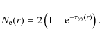
![]() .
In some tight binaries such as LS 5039, this gamma-ray absorption
mechanism is strong if the VHE emission occurs close to the compact
object. Gamma-ray absorption can account for an orbital modulation in
the VHE gamma-ray flux from LS 5039, as observed by HESS (Dubus 2006; Bednarek 2006; Böttcher & Dermer 2005).
.
In some tight binaries such as LS 5039, this gamma-ray absorption
mechanism is strong if the VHE emission occurs close to the compact
object. Gamma-ray absorption can account for an orbital modulation in
the VHE gamma-ray flux from LS 5039, as observed by HESS (Dubus 2006; Bednarek 2006; Böttcher & Dermer 2005).
A copious number of pairs may be produced in the surrounding medium as a by-product of the VHE gamma-ray absorption. If the number of pairs created is large enough and if they have enough time to radiate VHE photons before escaping, a sizeable electromagnetic cascade can be initiated. New generations of pairs and gamma rays are produced as long as the secondary particles have enough energy to boost stellar photons beyond the pair production threshold energy. Because of the anisotropic stellar photon field in the system, the inverse Compton radiation produced in the cascade has a strong angular dependence. The cascade contribution depends on the position of the primary gamma-ray source with respect to the massive star and a distant observer.
The VHE modulation in LS 5039 was explained in Dubus et al. (2008)
using phase-dependent absorption and inverse Compton emission, ignoring
the effect of pair cascading. This model did not predict any flux close
to superior conjunction, i.e. where the massive star lies between the compact object and the observer. This is contradicted by HESS observations (Aharonian et al. 2006a). Interestingly, this mismatch intervenes at phases where
![]() -opacity is known to be high
-opacity is known to be high
![]() .
The development of a cascade could contribute to the residual flux
observed in the system, with secondary gamma-ray emission filling in
for the highly absorbed primary gamma rays. This possibility has been
proposed to explain this discrepancy (Aharonian et al. 2006a) and is quantitatively investigated in this article.
.
The development of a cascade could contribute to the residual flux
observed in the system, with secondary gamma-ray emission filling in
for the highly absorbed primary gamma rays. This possibility has been
proposed to explain this discrepancy (Aharonian et al. 2006a) and is quantitatively investigated in this article.
The ambient magnetic field strength has a critical impact on the development of pair cascading. If the magnetic field strength is low enough to neglect the induced deflections on pair trajectories then the cascade develops along the line of sight joining the primary source of gamma rays and a distant observer. The particles do not radiate synchrotron radiation. Cascade calculations are then reduced to a one-dimension problem. Such a situation would apply in an unshocked pulsar wind where the pairs are cold relative to the magnetic field carried in the wind. This paper explores the development of an one-dimensional pair cascade in a binary and its implications.
Previous computations of cascade emission in binary environment were carried out by Bednarek (2007); Zdziarski et al. (2009); Bednarek (2006,1997); Sierpowska-Bartosik & Torres (2008); Aharonian et al. (2006b); Orellana et al. (2007); Sierpowska & Bednarek (2005); Khangulyan et al. (2008). Except for Aharonian et al. (2006b), all these works are based on Monte Carlo methods. One peculiarity of the gamma-ray binary environment is that the source of seed-photons for pair production and inverse Compton emission is the high luminosity companion star. This study proposes a semi-analytical model for one-dimensional cascades calculations, taking into account the anisotropy in the seed-photon field. The aim of the paper is to investigate and compute the total contribution from pair cascading in the system LS 5039, and see if it can account for the measured flux close to superior conjunction. The next section presents the main assumptions and equations for cascade computations. The development and the anisotropic effects of pair cascading in compact binaries are investigated. The density of escaping pairs and their rate of annihilation are also calculated in this part. The cascade contribution along the orbit in LS 5039 is computed and compared with the available observations in Sect. 3. The last section concludes on the implications of one-dimensional cascades in gamma-ray binaries. More details about pair production are available in the appendices.
2 Anisotropic pair cascading in compact binaries
2.1 Assumptions
This part examines one-dimensional cascading in the context of binary
systems. The massive star sets the seed-photon radiation field for the
cascade. For simplicity, the massive star is assumed point-like and
mono-energetic. This is a reasonable approximation as previous studies
on absorption (Dubus 2006) and emission (Dubus et al. 2008)
have shown. The effects of the magnetic field and pair annihilation are
neglected (see Sect. 2.5). Triplet pair production (TPP) due to
the high-energy electrons or positrons propagating in a soft photon
field (
![]() ,
Mastichiadis 1991) is not taken into account here. The cross section for this process becomes comparable to inverse Compton scattering when
,
Mastichiadis 1991) is not taken into account here. The cross section for this process becomes comparable to inverse Compton scattering when
![]() that is for electron energies
that is for electron energies
![]() TeV interacting with
TeV interacting with
![]() eV stellar photons. With a scattering rate of about
eV stellar photons. With a scattering rate of about ![]() 10-2
10-2
![]() ,
only a few pairs can be created via TPP by each VHE electron, before it
escapes or loses its energy in a Compton scattering. The created pairs
have much lower energy than the primary electrons. TPP cooling remains
inefficient compared to inverse Compton for VHE electrons with energy
,
only a few pairs can be created via TPP by each VHE electron, before it
escapes or loses its energy in a Compton scattering. The created pairs
have much lower energy than the primary electrons. TPP cooling remains
inefficient compared to inverse Compton for VHE electrons with energy ![]() PeV.
HESS observations of LS 5039 show a break in the spectrum at a few
TeV so few electrons are expected to interact by TPP in the cascade.
Observations of other gamma-ray binaries also show steep spectra but
this assumption will have to be revised if there is significant primary
emission beyond
PeV.
HESS observations of LS 5039 show a break in the spectrum at a few
TeV so few electrons are expected to interact by TPP in the cascade.
Observations of other gamma-ray binaries also show steep spectra but
this assumption will have to be revised if there is significant primary
emission beyond ![]() 10 TeV.
Pair production due to high-energy gamma rays interacting with the
surrounding material is also neglected. This occurs for
10 TeV.
Pair production due to high-energy gamma rays interacting with the
surrounding material is also neglected. This occurs for ![]() -rays >1 MeV and the cross-section is of order
-rays >1 MeV and the cross-section is of order
![]() (see e.g. Longair 1992), with
(see e.g. Longair 1992), with
![]() the Thomson cross-section. Since the measured
the Thomson cross-section. Since the measured ![]() is at most 1022 cm-2 in gamma-ray binaries, pair production on matter will not affect the propagation of gamma rays towards the observer.
is at most 1022 cm-2 in gamma-ray binaries, pair production on matter will not affect the propagation of gamma rays towards the observer.
Due to the high velocity of the center-of-mass (CM) frame in the
observer frame, the direction of propagation of pairs created by
![]() -absorption is boosted in the direction of the initial gamma ray. For a gamma ray of energy
-absorption is boosted in the direction of the initial gamma ray. For a gamma ray of energy
![]() TeV, the Lorentz factor of the CM to the observer frame transform is
TeV, the Lorentz factor of the CM to the observer frame transform is
![]() (see the Appendix, Eq. (A.2)). Pairs produced in the cascade are ultra-relativistic with typical Lorentz factor
(see the Appendix, Eq. (A.2)). Pairs produced in the cascade are ultra-relativistic with typical Lorentz factor
![]() .
Their emission is forward boosted within a cone of semi-aperture angle
.
Their emission is forward boosted within a cone of semi-aperture angle
![]() in the direction of electrons. The deviations on the electron trajectory due to scattering in the Thomson regime are
in the direction of electrons. The deviations on the electron trajectory due to scattering in the Thomson regime are ![]()
![]() .
In the Klein-Nishina regime most of the electron energy is given to the
photon. It is assumed here that electrons and photons produced in the
cascade remain on the same line, a good approximation since
.
In the Klein-Nishina regime most of the electron energy is given to the
photon. It is assumed here that electrons and photons produced in the
cascade remain on the same line, a good approximation since ![]() and
and
![]() .
This line joins the primary gamma-ray source to a distant observer (Fig. 1).
.
This line joins the primary gamma-ray source to a distant observer (Fig. 1).
Pair cascading is one-dimensional as long as magnetic deviations of
pairs trajectories along the Compton interaction length
![]() remain within the cone of emission of the electrons. This condition holds if
remain within the cone of emission of the electrons. This condition holds if
![]() ,
with
,
with ![]() the Larmor radius. For a typical interaction length
the Larmor radius. For a typical interaction length
![]() cm for TeV pairs in LS 5039, the ambient magnetic field must be lower than
cm for TeV pairs in LS 5039, the ambient magnetic field must be lower than
![]() G.
If the magnetic field strength is much greater, pairs locally
isotropize and radiate in all directions. In between, pairs follow the
magnetic field lines and the dynamics of each pairs must be followed as
treated in Sierpowska & Bednarek (2005).
The above limit may appear unrealistically stringent. However, since
deviations and isotropization will dilute the cascade flux, the
one-dimensional approach can be seen as maximizing the cascade
emission. More exactly, this redistribution induced by magnetic
deflections would decrease the cascade flux at orbital phases where
many pairs are produced to the benefit of phases where only a few are
created. Hence, the one-dimensional approach gives an upper limit to
the cascade contribution at phases where absorption is strong. If the
flux calculated here using this assumption is lower than required by
observations then cascading will be unlikely to play a role. Finally,
one-dimensional cascading should hold in the free pulsar wind as long
as the pairs move strictly along the magnetic field. In Sierpowska & Bednarek (2005) and Sierpowska-Bartosik & Torres (2008), the cascade radiation is computed up to the termination shock using a Monte Carlo approach. Sierpowska & Bednarek (2005)
also include a contribution from the region beyond the shock. The
cascade electrons in this region are assumed to follow the magnetic
field lines (in contrast with the pulsar wind zone where the
propagation is radial). There is no reacceleration at the shock and
synchrotron losses are neglected. In the method expounded here, the
cascade radiation is calculated semi-analytically from a point-like
gamma-ray source at the compact object location up to infinity,
providing the maximum possible contribution of the one-dimensional
cascade in gamma-ray binaries.
G.
If the magnetic field strength is much greater, pairs locally
isotropize and radiate in all directions. In between, pairs follow the
magnetic field lines and the dynamics of each pairs must be followed as
treated in Sierpowska & Bednarek (2005).
The above limit may appear unrealistically stringent. However, since
deviations and isotropization will dilute the cascade flux, the
one-dimensional approach can be seen as maximizing the cascade
emission. More exactly, this redistribution induced by magnetic
deflections would decrease the cascade flux at orbital phases where
many pairs are produced to the benefit of phases where only a few are
created. Hence, the one-dimensional approach gives an upper limit to
the cascade contribution at phases where absorption is strong. If the
flux calculated here using this assumption is lower than required by
observations then cascading will be unlikely to play a role. Finally,
one-dimensional cascading should hold in the free pulsar wind as long
as the pairs move strictly along the magnetic field. In Sierpowska & Bednarek (2005) and Sierpowska-Bartosik & Torres (2008), the cascade radiation is computed up to the termination shock using a Monte Carlo approach. Sierpowska & Bednarek (2005)
also include a contribution from the region beyond the shock. The
cascade electrons in this region are assumed to follow the magnetic
field lines (in contrast with the pulsar wind zone where the
propagation is radial). There is no reacceleration at the shock and
synchrotron losses are neglected. In the method expounded here, the
cascade radiation is calculated semi-analytically from a point-like
gamma-ray source at the compact object location up to infinity,
providing the maximum possible contribution of the one-dimensional
cascade in gamma-ray binaries.
![\begin{figure}
\par\includegraphics[width=8.5cm,clip]{12494fg1.eps}
\end{figure}](/articles/aa/full_html/2009/45/aa12494-09/img54.png)
|
Figure 1:
This diagram describes the system geometry. A gamma-ray photon of energy
|
| Open with DEXTER | |
2.2 Cascade equations
In order to compute the contribution from the cascade, the radiative transfer equation and the kinetic equation of the pairs have to be solved simultaneously.
The radiative transfer equation for the gamma-ray density
![]() at a distance r from the source is
at a distance r from the source is
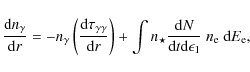
where
The kinetic equation for the pairs is given by the following integro-differential equation for
![]() (D'Avezac et al. 2007; Blumenthal & Gould 1970; Zdziarski 1988)
(D'Avezac et al. 2007; Blumenthal & Gould 1970; Zdziarski 1988)
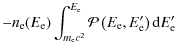
where
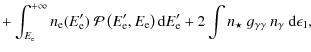
Since the inverse Compton kernel gives the probability per electron of energy ![]() to produce a gamma ray of energy
to produce a gamma ray of energy
![]() ,
the scattering rate can be rewritten as
,
the scattering rate can be rewritten as
The expression of
where
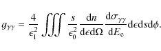
The anisotropic cascade can be computed by inserting the anisotropic
kernels for inverse Compton scattering (see Eq. (A.6) in Dubus et al. 2008) and for pair production obtained in Eq. (B.5) in Eqs. (1), (2).
The following sections present cascade calculations applied to compact
binaries, using a simple Runge-Kutta 4 integration method. It is more
convenient to perform integrations over an angular variable rather than
r. Here, calculations are carried out using ![]() ,
the angle between the line joining the massive star to the observation point and the line of sight (see Fig. 1).
,
the angle between the line joining the massive star to the observation point and the line of sight (see Fig. 1).
2.3 Cascade growth along the line of sight
Figure 2 presents cascade calculations for different distances r
from the primary gamma-ray source. For illustrative purpose, the source
is assumed isotropic and point-like, injecting a power-law distribution
of photons with an index -2 at r=0 but no electrons. The calculations were carried out for a system like LS 5039 and for a viewing angle
![]() .
In this geometric configuration, absorption is known to be strong (
.
In this geometric configuration, absorption is known to be strong (
![]() for 200 GeV photons) and a significant fraction of the total
absorbed energy is expected to be reprocessed in the cascade, inverse
Compton scattering being also very efficient in this configuration.
for 200 GeV photons) and a significant fraction of the total
absorbed energy is expected to be reprocessed in the cascade, inverse
Compton scattering being also very efficient in this configuration.
Close to the source (![]() with d the orbital separation), absorption produces a sharp and deep dip in the spectrum (light dashed line) but the cascade starts
to fill the gap (black solid line). The angle
with d the orbital separation), absorption produces a sharp and deep dip in the spectrum (light dashed line) but the cascade starts
to fill the gap (black solid line). The angle ![]() increases with the distance r
to the primary source. Hence, the threshold energy for pair production
increases as well. Cascading adds more flux to higher energy gamma rays
where absorption is maximum. The cascade produces an excess of low
energy gamma rays below the minimum threshold energy
increases with the distance r
to the primary source. Hence, the threshold energy for pair production
increases as well. Cascading adds more flux to higher energy gamma rays
where absorption is maximum. The cascade produces an excess of low
energy gamma rays below the minimum threshold energy
![]() GeV.
Because these new photons do not suffer from absorption, they
accumulate at lower energies. This is a well-known feature of
cascading.
GeV.
Because these new photons do not suffer from absorption, they
accumulate at lower energies. This is a well-known feature of
cascading.
2.4 Anisotropic effects
![\begin{figure}
\par\includegraphics[width=8cm,clip]{12494fg2.eps}
\end{figure}](/articles/aa/full_html/2009/45/aa12494-09/img82.png)
|
Figure 2: Cascade development along
the path to the observer. The primary source of photons, situated at
the location of the compact object, has a power law spectral
distribution with photon index -2
(dotted line). Spectra are computed using the parameters appropriate
for LS 5039 at superior conjunction (
|
| Open with DEXTER | |
![\begin{figure}
\par\includegraphics[width=15.7cm,clip]{12494fg3.eps}
\end{figure}](/articles/aa/full_html/2009/45/aa12494-09/img83.png)
|
Figure 3: Spectra as seen by an
observer at infinity, taking into account the effect of cascading.
Calculations are applied to LS 5039 at periastron for different
viewing angle
|
| Open with DEXTER | |
The left panel in Fig. 3
shows the complete spectrum taking into account cascading (solid line)
compared to the pure absorbed power-law (dashed line). Due to the
angular dependence in the pair production process, higher viewing
angles shift the cascade contribution to higher energies and decrease
its amplitude (Fig. 3, right panel). The cascade flux is low enough to be ignored for
![]() .
.
Three different zones can be distinguished in the cascade spectra.
First, below the pair production threshold energy, photons accumulate
in a low energy tail (photon index ![]() -1.5) produced by inverse Compton cooling of pairs. For
-1.5) produced by inverse Compton cooling of pairs. For
![]() ,
a low energy cut-off is observed due to the pairs escaping the system (Cerutti et al. 2008; Ball & Kirk 2000). This low energy cut-off is at about 0.1 GeV for
,
a low energy cut-off is observed due to the pairs escaping the system (Cerutti et al. 2008; Ball & Kirk 2000). This low energy cut-off is at about 0.1 GeV for
![]() .
The cutoff occurs when the cascade reaches a distance from the primary source corresponding to
.
The cutoff occurs when the cascade reaches a distance from the primary source corresponding to
![]() .
Then, the electrons cannot cool effectively because the inverse Compton
interaction angle diminishes and the stellar photon density decreases
as they propagate. For
.
Then, the electrons cannot cool effectively because the inverse Compton
interaction angle diminishes and the stellar photon density decreases
as they propagate. For
![]() ,
particles escape right away from the vicinity of the companion star and
no tail is produced. Second, above the threshold energy, there is a
competition between absorption and gamma-ray production by reprocessed
pairs, particularly for low angles where both effects are strong. Even
if cascading increases the transparency for gamma rays, absorption
still creates a dip in the spectrum. Third, well beyond the threshold
energy, absorption becomes inefficient. Fewer pairs are created,
producing a high-energy cut-off (
,
particles escape right away from the vicinity of the companion star and
no tail is produced. Second, above the threshold energy, there is a
competition between absorption and gamma-ray production by reprocessed
pairs, particularly for low angles where both effects are strong. Even
if cascading increases the transparency for gamma rays, absorption
still creates a dip in the spectrum. Third, well beyond the threshold
energy, absorption becomes inefficient. Fewer pairs are created,
producing a high-energy cut-off (![]() 10 TeV, for
10 TeV, for
![]() ). Klein-Nishina effects also contribute to the decrease of the high-energy gamma-rays production.
). Klein-Nishina effects also contribute to the decrease of the high-energy gamma-rays production.
2.5 Escaping pairs
The spectrum of pairs produced in the cascade as seen at infinity is shown in Fig. 4. The density depends strongly on the viewing angle as expected, but the mean energy of pairs lies at very high energies (
![]() GeV, see Table 1). The accumulation of very high-energy particles can be explained by two concurrent effects. Far from the massive star (
GeV, see Table 1). The accumulation of very high-energy particles can be explained by two concurrent effects. Far from the massive star (![]() ),
most of the pairs are created at very high energy due to the high
threshold energy (almost rear-end collision). The second effect is that
inverse Compton losses are in deep Klein-Nishina regime for high-energy
electrons. The cooling timescale increases and becomes longer than the
propagation timescale of electrons close to the companion star,
producing an accumulation of pairs at very high energies.
),
most of the pairs are created at very high energy due to the high
threshold energy (almost rear-end collision). The second effect is that
inverse Compton losses are in deep Klein-Nishina regime for high-energy
electrons. The cooling timescale increases and becomes longer than the
propagation timescale of electrons close to the companion star,
producing an accumulation of pairs at very high energies.
The distribution of pairs allows to assess the fraction of the
total absorbed energy escaping the system in the form of kinetic energy
in the pairs. This non-radiated power ![]() can be compared to the radiated power released in the cascade
can be compared to the radiated power released in the cascade ![]() .
Energy conservation yields the total absorbed power
.
Energy conservation yields the total absorbed power
![]() .
.
![\begin{figure}
\par\includegraphics[width=7.7cm,clip]{12494fg4.eps}
\end{figure}](/articles/aa/full_html/2009/45/aa12494-09/img93.png)
|
Figure 4:
Distribution of escaping pairs seen by a distant observer, depending on the viewing angle
|
| Open with DEXTER | |
Table 1: Mean energy of escaping pairs and radiated power efficiency of the cascade.
The asymptotic radiated power reached by the cascade is compared to the
total absorbed power integrated over energy in Table 1. The fraction of lost energy increases with the viewing angle. In fact, for
![]() most of the power remains in kinetic energy. Once the electrons are
created, only a few have time to radiate through inverse Compton
interaction. Below (
most of the power remains in kinetic energy. Once the electrons are
created, only a few have time to radiate through inverse Compton
interaction. Below (
![]() ), the radiative power dominates and the cascade is very efficient (recycling efficiency up to 80% for
), the radiative power dominates and the cascade is very efficient (recycling efficiency up to 80% for
![]() ). The cascade is fully linear, since the power re-radiated remains much lower than the star luminosity
). The cascade is fully linear, since the power re-radiated remains much lower than the star luminosity
![]() (Svensson 1987). Self-interactions in the cascade are then negligible. This is also a consequence of Klein-Nishina cascading (Zdziarski 1988). In addition, interactions between particles in the cascade would be forcedly rear-end, hence highly inefficient.
(Svensson 1987). Self-interactions in the cascade are then negligible. This is also a consequence of Klein-Nishina cascading (Zdziarski 1988). In addition, interactions between particles in the cascade would be forcedly rear-end, hence highly inefficient.
The created positrons will annihilate and form a 511 keV
line. However, the expected signal is very weak. The annihilation
cross-section is
![]() (see e.g. Longair 1992). The escaping positrons have a very high average Lorentz factor
(see e.g. Longair 1992). The escaping positrons have a very high average Lorentz factor
![]() (Table 1)
so they are unlikely to annihilate within the system. They will
thermalize and annihilate in the interstellar medium. Escaping
positrons from gamma-ray binaries are unlikely to contribute much to
the diffuse 511 keV emission. The average number of pairs created along
the orbit in LS 5039 (based on the results to be discussed in the
following section) is
(Table 1)
so they are unlikely to annihilate within the system. They will
thermalize and annihilate in the interstellar medium. Escaping
positrons from gamma-ray binaries are unlikely to contribute much to
the diffuse 511 keV emission. The average number of pairs created along
the orbit in LS 5039 (based on the results to be discussed in the
following section) is
![]() .
This estimate does not take into account contributions from triplet
pair production or from the pulsar wind (for a pulsar injecting pairs
with
.
This estimate does not take into account contributions from triplet
pair production or from the pulsar wind (for a pulsar injecting pairs
with
![]() and a luminosity of
and a luminosity of
![]() ,
about
,
about
![]() pairs are produced). Gamma-ray binaries have short lifetimes and it is
unlikely there is more than a few hundred currently active in the
Galaxy. Hence, the expected contribution is orders-of-magnitude below
the positron flux required to explain the diffuse 511 keV emission
(
pairs are produced). Gamma-ray binaries have short lifetimes and it is
unlikely there is more than a few hundred currently active in the
Galaxy. Hence, the expected contribution is orders-of-magnitude below
the positron flux required to explain the diffuse 511 keV emission
(![]()
![]() ,
Knödlseder et al. 2005). Even
if the positrons thermalize close to or within the system (because
magnetic fields contain them, see Sect. 5) then, following Guessoum et al. (2006), the expected contribution from a single source at 2 kpc would be at most
,
Knödlseder et al. 2005). Even
if the positrons thermalize close to or within the system (because
magnetic fields contain them, see Sect. 5) then, following Guessoum et al. (2006), the expected contribution from a single source at 2 kpc would be at most ![]() 10-9 ph cm-2 s-1, which is currently well below detectability.
10-9 ph cm-2 s-1, which is currently well below detectability.
3 Cascading in LS 5039
![\begin{figure}
\par\includegraphics[width=7.7cm,clip]{12494fg5.eps}
\end{figure}](/articles/aa/full_html/2009/45/aa12494-09/img107.png)
|
Figure 5:
Orbit-averaged spectra in LS 5039 at INFC (
|
| Open with DEXTER | |
![\begin{figure}
\par\includegraphics[width=7.7cm,clip]{12494fg6.eps}
\end{figure}](/articles/aa/full_html/2009/45/aa12494-09/img108.png)
|
Figure 6:
Computed light-curves along the orbit in LS 5039, in the HESS energy band (flux |
| Open with DEXTER | |
LS 5039 was detected by HESS (Aharonian et al. 2005) and the orbital modulation of the TeV gamma-ray flux was later on reported in Aharonian et al. (2006a).
Most of the temporal and spectral features can be understood as a
result of anisotropic gamma-ray absorption and emission from
relativistic electrons accelerated in the immediate vicinity of the
compact object, e.g. in the pulsar wind termination shock (Dubus et al. 2008).
However, this description fails to explain the residual flux observed
close to superior conjunction where a significant excess has been
detected (6.1![]() at phase
at phase
![]() ).
The primary gamma rays should be completely attenuated. The aim of this
part is to find if cascading can account for this observed flux. The
cascade is assumed to develop freely from the primary gamma-ray source
up to the observer. The contribution of the cascade as a function of
the orbital phase is also investigated.
).
The primary gamma rays should be completely attenuated. The aim of this
part is to find if cascading can account for this observed flux. The
cascade is assumed to develop freely from the primary gamma-ray source
up to the observer. The contribution of the cascade as a function of
the orbital phase is also investigated.
The primary source of gamma rays now considered is the spectrum calculated in Dubus et al. (2008).
Figure 5 shows phase-averaged spectra along the orbit at INFC (orbital phase
![]() )
and SUPC (
)
and SUPC (![]() or
or ![]() )
for the primary source, the cascade and the sum of both components. The
orbital parameters and the distance (2.5 kpc) are taken from Casares et al. (2005) for an inclination
)
for the primary source, the cascade and the sum of both components. The
orbital parameters and the distance (2.5 kpc) are taken from Casares et al. (2005) for an inclination
![]() so
so ![]() varies between
varies between
![]() .
The cascade contribution is highly variable along the orbit and dominates
at SUPC for
.
The cascade contribution is highly variable along the orbit and dominates
at SUPC for
![]() GeV,
where a high pair-production rate is expected. At INFC, cascading is
negligible compared with the primary flux. With pair cascading the
spectral differences between INFC and SUPC are very small at VHE,
contrary to what is observed by HESS. In the GeV band, cascades
contribute to a spectral hardening at SUPC close to 10-30 GeV.
GeV,
where a high pair-production rate is expected. At INFC, cascading is
negligible compared with the primary flux. With pair cascading the
spectral differences between INFC and SUPC are very small at VHE,
contrary to what is observed by HESS. In the GeV band, cascades
contribute to a spectral hardening at SUPC close to 10-30 GeV.
Orbital light-curves in the HESS energy band give a better appreciation of the contribution from both components (Fig. 6). The contribution from cascading is anti-correlated with the primary absorbed flux. The cascade light-curve
is minimum at inferior conjunction (
![]() ).
The non trivial double peaked structure of the lightcurve at phases
0.85-0.35 is due to competition in the cascade between absorption and
inverse Compton emission. Absorption has a slight edge at superior
conjunction (
).
The non trivial double peaked structure of the lightcurve at phases
0.85-0.35 is due to competition in the cascade between absorption and
inverse Compton emission. Absorption has a slight edge at superior
conjunction (
![]() ), producing a dip at this phase.
Elsewhere, the primary contribution dominates over the cascade emission.
At lower energies (
), producing a dip at this phase.
Elsewhere, the primary contribution dominates over the cascade emission.
At lower energies (
![]() GeV), the cascade contribution is undistinguishable from the primary source.
GeV), the cascade contribution is undistinguishable from the primary source.
In this configuration, the cascade does add VHE gamma-ray
emission close to superior conjunction but the expected contribution
overestimates HESS observations. Decreasing the inclination of the
system does not help: the cascade flux in the TeV energy band
increases, since the primary source is on average more absorbed along
the orbit (see Sect. 3 in Dubus 2006). For
![]() ,
the cascade contribution dominates the primary flux at every orbital phases in the VHE band.
One-dimension cascades can be ruled out by the current HESS observations of LS 5039.
,
the cascade contribution dominates the primary flux at every orbital phases in the VHE band.
One-dimension cascades can be ruled out by the current HESS observations of LS 5039.
4 Conclusion
This paper explored the impact of one-dimensional pair cascading on the formation of the very high-energy radiation from gamma-ray binaries in general, LS 5039 specifically. A significant fraction of the total absorbed energy can be reprocessed at lower energy by the cascade, decreasing the global opacity of the primary source. Anisotropic effects also play a major role on the cascade radiation spectrum seen by a distant observer.
A large contribution from cascading is expected in
LS 5039, large enough that it significantly overestimates the flux
observed by HESS. One-dimensional cascading is too efficient in
redistributing the absorbed primary flux and can be ruled out. However,
the fact that it overestimates the observed flux means a more general
cascade cannot be ruled out (it would have been if the HESS flux had
been underestimated). If the ambient magnetic field is high enough (
![]() G) the pairs will be deflected from the line-of-sight. For
G) the pairs will be deflected from the line-of-sight. For
![]() G
the Larmor radius of a TeV electron becomes smaller than the
LS 5039 orbital separation and the pairs will be more and more
isotropized locally. All of this will tend to dilute cascade emission
compared to the one-dimensional case, which should therefore be seen as
an upper limit to the cascade contribution at orbital phases where
absorption is strong, particularly at superior conjunction. The
initiated cascade will be three-dimensional as pointed out by Bednarek (1997).
Each point in the binary system becomes a potential secondary source
able to contribute to the total gamma-ray flux at every orbital phases.
Cascade emission can still be sizeable all along the orbit in
LS 5039, yet form a more weakly modulated background in the
light-curve on account of the cascade radiation redistribution at other
phases. The strength and structure of the surrounding magnetic field
(from both stars) has a strong influence on the cascade (Bosch-Ramon et al. 2008b; Sierpowska & Bednarek 2005; Bosch-Ramon et al. 2008a).
More realistic pair cascading calculations cannot be treated with the
semi-analytical approach exposed here. Complementary investigations
using a Monte Carlo approach are needed to better appreciate the
cascade contribution in gamma-ray binaries.
G
the Larmor radius of a TeV electron becomes smaller than the
LS 5039 orbital separation and the pairs will be more and more
isotropized locally. All of this will tend to dilute cascade emission
compared to the one-dimensional case, which should therefore be seen as
an upper limit to the cascade contribution at orbital phases where
absorption is strong, particularly at superior conjunction. The
initiated cascade will be three-dimensional as pointed out by Bednarek (1997).
Each point in the binary system becomes a potential secondary source
able to contribute to the total gamma-ray flux at every orbital phases.
Cascade emission can still be sizeable all along the orbit in
LS 5039, yet form a more weakly modulated background in the
light-curve on account of the cascade radiation redistribution at other
phases. The strength and structure of the surrounding magnetic field
(from both stars) has a strong influence on the cascade (Bosch-Ramon et al. 2008b; Sierpowska & Bednarek 2005; Bosch-Ramon et al. 2008a).
More realistic pair cascading calculations cannot be treated with the
semi-analytical approach exposed here. Complementary investigations
using a Monte Carlo approach are needed to better appreciate the
cascade contribution in gamma-ray binaries.
Finally, the cascade will be quenched if the created pairs lose
energy to synchrotron rather than inverse Compton scattering. This
requires ambient magnetic fields ![]() G,
as found by equating the radiative timescales for a 1 TeV electron
at periastron in LS 5039. Such ambient magnetic field strengths
could be reached close to the companion star. In this case an
alternative explanation is needed to account for the flux at superior
conjunction. A natural one to consider is that the primary gamma-ray
source is farther from the massive star. The VHE source would not be
coincident with the compact object location anymore and would suffer
less from absorption. In the microquasar scenario, Bednarek (2007)
can account for consistent flux with HESS observations at superior
conjunction if some electrons are injected well above the orbital plane
(jet altitude
G,
as found by equating the radiative timescales for a 1 TeV electron
at periastron in LS 5039. Such ambient magnetic field strengths
could be reached close to the companion star. In this case an
alternative explanation is needed to account for the flux at superior
conjunction. A natural one to consider is that the primary gamma-ray
source is farther from the massive star. The VHE source would not be
coincident with the compact object location anymore and would suffer
less from absorption. In the microquasar scenario, Bednarek (2007)
can account for consistent flux with HESS observations at superior
conjunction if some electrons are injected well above the orbital plane
(jet altitude
![]() ). In addition to LS 5039, this possibility was also considered for the system Cyg X-1 by Bosch-Ramon et al. (2008b) and Zdziarski et al. (2009).
). In addition to LS 5039, this possibility was also considered for the system Cyg X-1 by Bosch-Ramon et al. (2008b) and Zdziarski et al. (2009).
In practice, reality may consist of a complex three-dimensional cascade partly diluted and partly quenched depending upon position, angle and magnetic field configuration.
AcknowledgementsG.D. thanks A. Mastichiadis for discussions of triplet pair production. This work was supported by the European Community via contract ERC-StG-200911.
Appendix A: Pair production
The main equations for the pair production process are briefly presented here. Detailed calculations can be found in Gould & Schréder (1967), Bonometto & Rees (1971) and Böttcher & Schlickeiser (1997).
A.1 Kinematics and cross-sections
The interaction of a gamma-ray photon of energy
![]() and a soft photon of energy
and a soft photon of energy
![]() in
the observer frame leads to the production of an electron-positron pair
if the total available energy in the center-of-mass (CM) frame is
greater than the rest mass energy of the pair
in
the observer frame leads to the production of an electron-positron pair
if the total available energy in the center-of-mass (CM) frame is
greater than the rest mass energy of the pair
where
The differential cross-section
![]() in the CM frame depends on
in the CM frame depends on ![]() and the angle
and the angle ![]() between the outcoming electron-positron pair and the incoming photons. The full expression can be found in e.g. Bonometto & Rees (1971), Eq. (2.7). The differential cross-section presents a symmetric structure, peaked at
between the outcoming electron-positron pair and the incoming photons. The full expression can be found in e.g. Bonometto & Rees (1971), Eq. (2.7). The differential cross-section presents a symmetric structure, peaked at
![]() and minimum for
and minimum for
![]() .
Electrons are mostly created in the same and opposite direction with
respect to the incoming hard photon direction in the CM frame. The
double peaked structure is enhanced with increasing energy (
.
Electrons are mostly created in the same and opposite direction with
respect to the incoming hard photon direction in the CM frame. The
double peaked structure is enhanced with increasing energy (
![]() )
and becomes less pronounced close to the threshold (
)
and becomes less pronounced close to the threshold (
![]() ). The integration over the angles gives the total pair production cross-section
). The integration over the angles gives the total pair production cross-section
![]() ,
maximum close to the threshold (see Eq. (1) in Gould & Schréder 1967).
,
maximum close to the threshold (see Eq. (1) in Gould & Schréder 1967).
The construction of the CM frame with respect to the observer
frame can be simplified if one of the incoming photons carries most of
the energy. This case is appropriate in the present context. For
![]() ,
the CM frame can be considered as propagating along the same direction
as the high-energy photon. The velocity of the CM frame in the observer
frame can be expressed as
,
the CM frame can be considered as propagating along the same direction
as the high-energy photon. The velocity of the CM frame in the observer
frame can be expressed as
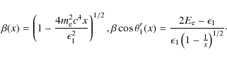
The total energy of say the electron
![\begin{displaymath}E_{\rm e}=\gamma'\left[s^{1/2}+\beta'\left(s-m_{\rm e}^2 c^4\right)^{1/2}\cos\theta'_1\right],
\end{displaymath}](/articles/aa/full_html/2009/45/aa12494-09/img138.png)
providing a relation between
A.2 Rate of absorption and pair spectrum kernels
A gamma-ray photon going through a soft photon gas of density
![]() is absorbed at a rate per unit of path length l
is absorbed at a rate per unit of path length l
The absorption rate gives the probability for a gamma ray of energy
Following Bonometto & Rees (1971), the probability for a gamma ray of energy
![]() to be absorbed between l and
to be absorbed between l and
![]() yielding an electron of energy between
yielding an electron of energy between ![]() and
and
![]() (with a positron of energy
(with a positron of energy
![]() for
for
![]() )
is
)
is
As with anisotropic inverse Compton scattering (Dubus et al. 2008), it is useful to consider the case of a monoenergetic beam of soft photons. The normalized soft photon density in the observer frame is
where
The anisotropic kernel integrated over all the pitch angles, in the
case of an isotropic gas of photons, is consistent with the kernel
found by Aharonian et al. (1983). Note that a general expression for the anisotropic kernel valid beyond the approximation
![]() is presented in Böttcher & Schlickeiser (1997).
is presented in Böttcher & Schlickeiser (1997).
A.3 Pair density
The number of pair created per unit of length path and electron energy
depends on the probability to create a pair and on the probability for
the incoming gamma ray to remain unabsorbed up to the point of
observation so that
Because of the symmetry in
The total number of pairs produced by a single gamma ray bathed in a soft radiation along the path l up to the distance r is then
For low opacity
Appendix B: Anisotropic pair production kernel
![\begin{figure}
\par\includegraphics[width=7.5cm,clip]{12494fg7.eps}
\end{figure}](/articles/aa/full_html/2009/45/aa12494-09/img159.png)
|
Figure B.1:
Anisotropic pair production kernel
|
| Open with DEXTER | |
Combining the expression of
The differential cross-section can then be expressed as
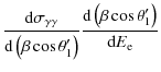
The complete general formula to compute the spectrum of the pair for a non-specified soft radiation field is
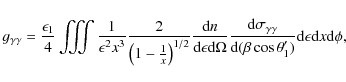
corresponding to Eq. (2.14) in Bonometto & Rees (1971). The injection of a mono-energetic and unidirectional soft photon density (Eq. (A.6)) in this last equation yields
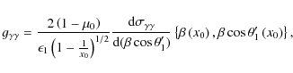
where
This expression is valid for
![\begin{displaymath}E_{\pm}=\frac{\epsilon_1}{2}\left[1\pm\left(1-\frac{1}{x_0}\r...
...{4 m_{\rm e}^2 c^4 x_0}{\epsilon^2_1}\right)^{1/2}\right]\cdot
\end{displaymath}](/articles/aa/full_html/2009/45/aa12494-09/img170.png)
Figure B.1 presents the pair production kernel for different incoming gamma-ray energy
Note that a kernel can be calculated as well for the absorption rate. Injecting Eqs. (A.6) into (A.4) is straightforward and gives
References
- Aharonian, F., Akhperjanian, A. G., Aye, K.-M., et al. 2005, Science, 309, 746 [NASA ADS] [CrossRef]
- Aharonian, F. A., Atoian, A. M., & Nagapetian, A. M. 1983, Astrofizika, 19, 323 [NASA ADS]
- Aharonian, F., Akhperjanian, A. G., Bazer-Bachi, A. R., et al. 2006a, A&A, 460, 743 [NASA ADS] [CrossRef] [EDP Sciences]
- Aharonian, F., Anchordoqui, L., Khangulyan, D., & Montaruli, T. 2006b, J. Phys. Conf. Ser., 39, 408 [NASA ADS] [CrossRef]
- Ball, L., & Kirk, J. G. 2000, Astropart. Phys., 12, 335 [NASA ADS] [CrossRef]
- Bednarek, W. 1997, A&A, 322, 523 [NASA ADS]
- Bednarek, W. 2006, MNRAS, 368, 579 [NASA ADS] [CrossRef]
- Bednarek, W. 2007, A&A, 464, 259 [NASA ADS] [CrossRef] [EDP Sciences]
- Blumenthal, G. R., & Gould, R. J. 1970, Rev. Mod. Phys., 42, 237 [NASA ADS] [CrossRef]
- Bonometto, S., & Rees, M. J. 1971, MNRAS, 152, 21 [NASA ADS]
- Bosch-Ramon, V., Khangulyan, D., & Aharonian, F. A. 2008a, A&A, 482, 397 [NASA ADS] [CrossRef] [EDP Sciences]
- Bosch-Ramon, V., Khangulyan, D., & Aharonian, F. A. 2008b, A&A, 489, L21 [NASA ADS] [CrossRef] [EDP Sciences]
- Böttcher, M., & Dermer, C. D. 2005, ApJ, 634, L81 [NASA ADS] [CrossRef]
- Böttcher, M., & Schlickeiser, R. 1997, A&A, 325, 866 [NASA ADS]
- Casares, J., Ribó, M., Ribas, I., et al. 2005, MNRAS, 364, 899 [NASA ADS] [CrossRef]
- Cerutti, B., Dubus, G., & Henri, G. 2008, A&A, 488, 37 [NASA ADS] [CrossRef] [EDP Sciences]
- D'Avezac, P., Dubus, G., & Giebels, B. 2007, A&A, 469, 857 [NASA ADS] [CrossRef] [EDP Sciences]
- Dubus, G. 2006, A&A, 451, 9 [NASA ADS] [CrossRef] [EDP Sciences]
- Dubus, G., Cerutti, B., & Henri, G. 2008, A&A, 477, 691 [NASA ADS] [CrossRef] [EDP Sciences]
- Gould, R. J., & Schréder, G. P. 1967, Phys. Rev., 155, 1408 [NASA ADS] [CrossRef]
- Guessoum, N., Jean, P., & Prantzos, N. 2006, A&A, 457, 753 [NASA ADS] [CrossRef] [EDP Sciences]
- Hartman, R. C., Bertsch, D. L., Bloom, S. D., et al. 1999, ApJS, 123, 79 [NASA ADS] [CrossRef]
- Khangulyan, D., Aharonian, F., & Bosch-Ramon, V. 2008, MNRAS, 383, 467 [NASA ADS]
- Knödlseder, J., Jean, P., Lonjou, V., et al. 2005, A&A, 441, 513 [NASA ADS] [CrossRef] [EDP Sciences]
- Longair, M. S. 1992, High energy astrophysics, Vol. 1: particles, photons and their detection, ed. M. S. Longair
- Mastichiadis, A. 1991, MNRAS, 253, 235 [NASA ADS]
- Orellana, M., Bordas, P., Bosch-Ramon, V., Romero, G. E., & Paredes, J. M. 2007, A&A, 476, 9 [NASA ADS] [CrossRef] [EDP Sciences]
- Rybicki, G. B., & Lightman, A. P. 1979, Radiative processes in astrophysics (New York: Wiley-Interscience), 393
- Sierpowska, A., & Bednarek, W. 2005, MNRAS, 356, 711 [NASA ADS] [CrossRef]
- Sierpowska-Bartosik, A., & Torres, D. F. 2008, Astropart. Phys., 30, 239 [NASA ADS] [CrossRef]
- Svensson, R. 1987, MNRAS, 227, 403 [NASA ADS]
- Zdziarski, A. A. 1988, ApJ, 335, 786 [NASA ADS] [CrossRef]
- Zdziarski, A. A. 1989, ApJ, 342, 1108 [NASA ADS] [CrossRef]
- Zdziarski, A. A., Malzac, J., & Bednarek, W. 2009, MNRAS, L175
All Tables
Table 1: Mean energy of escaping pairs and radiated power efficiency of the cascade.
All Figures
|
|
Figure 1:
This diagram describes the system geometry. A gamma-ray photon of energy
|
| Open with DEXTER | |
| In the text | |
|
|
Figure 2: Cascade development along
the path to the observer. The primary source of photons, situated at
the location of the compact object, has a power law spectral
distribution with photon index -2
(dotted line). Spectra are computed using the parameters appropriate
for LS 5039 at superior conjunction (
|
| Open with DEXTER | |
| In the text | |
|
|
Figure 3: Spectra as seen by an
observer at infinity, taking into account the effect of cascading.
Calculations are applied to LS 5039 at periastron for different
viewing angle
|
| Open with DEXTER | |
| In the text | |
|
|
Figure 4:
Distribution of escaping pairs seen by a distant observer, depending on the viewing angle
|
| Open with DEXTER | |
| In the text | |
|
|
Figure 5:
Orbit-averaged spectra in LS 5039 at INFC (
|
| Open with DEXTER | |
| In the text | |
|
|
Figure 6:
Computed light-curves along the orbit in LS 5039, in the HESS energy band (flux |
| Open with DEXTER | |
| In the text | |
|
|
Figure B.1:
Anisotropic pair production kernel
|
| Open with DEXTER | |
| In the text | |
Copyright ESO 2009
Current usage metrics show cumulative count of Article Views (full-text article views including HTML views, PDF and ePub downloads, according to the available data) and Abstracts Views on Vision4Press platform.
Data correspond to usage on the plateform after 2015. The current usage metrics is available 48-96 hours after online publication and is updated daily on week days.
Initial download of the metrics may take a while.