| Issue |
A&A
Volume 507, Number 3, December I 2009
|
|
|---|---|---|
| Page(s) | 1711 - 1718 | |
| Section | Astronomical instrumentation | |
| DOI | https://doi.org/10.1051/0004-6361/200912467 | |
| Published online | 01 October 2009 | |
A&A 507, 1711-1718 (2009)
Nonlinear deconvolution with deblending: a new analyzing technique for spectroscopy
C. Sennhauser1 - S. V. Berdyugina1,2 - D. M. Fluri1
1 - Institute for Astronomy, ETH Zurich, 8093 Zurich, Switzerland
2 - Kiepenheuer Institut für Sonnenphysik, 79104 Freiburg, Germany
Received 11 May 2009 / Accepted 1 August 2009
Abstract
Context. Spectroscopy data in general often deals with an
entanglement of spectral line properties, especially in the case of
blended line profiles, independently of how high the quality of the
data may be. In stellar spectroscopy and spectropolarimetry, where
atomic transition parameters are usually known, the use of multi-line
techniques to increase the signal-to-noise ratio of observations has
become common practice. These methods extract an average line profile
by means of either least squares deconvolution (LSD) or principle
component analysis (PCA). However, only a few methods account for the
blending of line profiles, and when they do, they assume that line
profiles add linearly.
Aims. We abandon the simplification of linear line-adding for Stokes I
and present a novel approach that accounts for the nonlinearity in
blended profiles, also illuminating the process of a reasonable
deconvolution of a spectrum. Only the combination of those two enables
us to treat spectral line variables independently, constituting our
method of nonlinear deconvolution with deblending (NDD). The improved
interpretation of a common line profile achieved compensates for the
additional expense in calculation time, especially when it comes to the
application to (Zeeman) doppler imaging (ZDI).
Methods. By examining how absorption lines of different depths
blend with each other and describing the effects of line-adding in a
mathematically simple, yet physically meaningful way, we discover how
it is possible to express a total line depth in terms of a (nonlinear)
combination of contributing individual components. Thus, we disentangle
blended line profiles and underlying parameters in a truthful manner
and strongly increase the reliability of the common line patterns
retrieved.
Results. By comparing different versions of LSD with our NDD
technique applied to simulated atomic and molecular intensity spectra,
we are able to illustrate the improvements provided by our method to
the interpretation of the recovered mean line profiles. As a
consequence, it is possible for the first time to retrieve an intrinsic
line pattern from a molecular band, offering the opportunity to fully
include them in a NDD-based ZDI. However, we also show that strong line
broadening deters the existence of a unique solution for heavily
blended lines such as in molecular bandheads.
Key words: line: formation - stars: magnetic fields
1 Introduction
A multi-line approach for increasing the signal-to-noise (S/N) ratio of measured line profiles was first introduced by Semel (1989) and Semel & Li (1996). It was developed into the LSD method by Donati et al. (1997).
The aim of these methods is to determine the common Stokes profiles of
polarized spectra when assuming the weak-field regime. It is assumed
that the line profiles are the same for all lines in the spectrum
except for a factor, which is given by the properties of the transition
![]() ,
i.e., wavelength, effective Landé factor, and oscillator strength, and
by the stellar atmosphere in which the lines form, i.e., shape and
depth of the (intensity) line. These mean Stokes profiles are called
common line patterns, or Zeeman patterns
,
i.e., wavelength, effective Landé factor, and oscillator strength, and
by the stellar atmosphere in which the lines form, i.e., shape and
depth of the (intensity) line. These mean Stokes profiles are called
common line patterns, or Zeeman patterns
![]() of a spectrum, which are presented in velocity space. The spectrum is
then a correlation of this common line pattern with a linemask, which
defines the line position (wavelength) and scaling in intensity.
Another approach is that of principal component analysis (PCA), where
denoising is achieved by diagonalizing a cross-product matrix of
individual spectral lines to reconstruct the data with a truncated
basis of eigenvectors (e.g., Martínez Gonzáles et al. 2008).
of a spectrum, which are presented in velocity space. The spectrum is
then a correlation of this common line pattern with a linemask, which
defines the line position (wavelength) and scaling in intensity.
Another approach is that of principal component analysis (PCA), where
denoising is achieved by diagonalizing a cross-product matrix of
individual spectral lines to reconstruct the data with a truncated
basis of eigenvectors (e.g., Martínez Gonzáles et al. 2008).
Methods such as LSD and PCA can be assumed to be filtering methods, which extract common line patterns of Stokes I,Q,U, and V in more detail, thus enabling a more precise description of the stellar atmosphere in which the lines formed, including the temperature and both the strength and orientation of the magnetic fields. For the task of Zeeman doppler imaging (ZDI), that reconstructs the brightness and magnetic field distribution on a stellar surface from input multiple exposures at different rotational phases, such a multi-line technique seems to be an appropriate tool for providing highly resolved information about the star merged in one single line profile.
To retrieve this common line pattern, it is insufficient to represent a spectrum as an accumulation of separate spectral lines, but it is necessary to deconvolve blended line profiles, i.e., to account for the contributions of closely neighbouring lines (in all Stokes parameters). So far, LSD methods assume that contributions from different lines add up linearly for all Stokes parameters, i.e., that the spectrum is a true convolution in a mathematical sense. We show that this is only valid for weak absorption lines, and we present a self-consistent way of analyzing arbitrary line depths. The main goal was to find a formalism that describes how line depths ``add'' in a physical sense, which we found in terms of the interpolation formula by Minnaert (1935), introduced for quite a different purpose.
In this paper, we consider intensity spectra only, while a consistent procedure for polarized spectra will be developed in a forthcoming paper. The paper is structured as follows. In Sect. 2, we consider the basics of multi-line techniques, introducing the principles of deblending. We then compare optically thin and thick cases in Sect. 3, to develop a general formalism from which we derive our nonlinear deconvolution with deblending (NDD) technique. The numerical implementation of our new method is given in Sect. 4, which is supplemented by Appendices A-C, where we provide details about inverse interpolation, solving algorithms, and defining the Jacobi matrix explicitly. A comparison of linear and nonlinear deconvolution, applied to simulated atomic and molecular lines is presented in Sect. 5. Finally, in Sect. 6, we summarize our conclutions.
2 Weak line decorrelation and deblending
We first consider how to extract a proportionality function (Zeeman
pattern) that is constant for all lines in a given intensity spectrum.
It is obvious that if we assume similar line profiles, i.e. no
saturation effects, each line profile is given by the characteristic
Zeeman pattern, which we choose to have a central line depth of 1,
``scaled'' by the central line depth
![]() of the current line i. For the surrounding local line profile
of the current line i. For the surrounding local line profile
![]() ,
however, it is more appropriate to consider
,
however, it is more appropriate to consider
rather than
|
(2) |
where vi and mI,i are respectively the position in velocity space and weight of each spectral line. To be able to write Eq. (1) in terms of a linemask, we complete the transformations
In the weak line approximation, a spectrum can be written in terms of a correlation expression of the so-called line pattern function, or linemask M, with the sought-after common line pattern Z,
| (4) |
As proposed by Donati et al. (1997), this is equivalent to a (linear) system of equations
If we know the error
If the pixel errors are unknown, S can be chosen to be the identity matrix and therefore omitted. In our discussion, we do not consider the error matrix, but do remember that if provided, it is important to include it during all further steps.
It should be emphasized here that for intensity spectra, the transformations given by Eq. (3) must be made prior to applying Eq. (5), because for Stokes I the normalized continuum equals 1, instead of zero as for V,Q, and U.
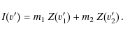
It is common to interpret Eq. (5) in terms of evaluating the common line pattern only for one single bin v' of a given velocity grid at a time, i.e., by transforming local line profiles
![]() for each line i=1,...,n into velocity space with their line centers as origin and defining a system of n equations
for each line i=1,...,n into velocity space with their line centers as origin and defining a system of n equations
In this approach, M and I are one-dimensional arrays, and inserting them into Eq. (5) yields the least squares solution of one element of ZI at a given velocity grid point. Equations (6) assume that there are no blended lines or more precisely that there is only a contribution to Z from one line at a time. The effect of blends is assumed to be averaged statistically. However, in general a measurement at wavelength
where v'i is the velocity distance measured from the line center
|
(8) |
The equation for the next pixel at
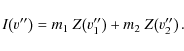
|
(9) |
For some additional pixel at
| (10) |
This approach not only deconvolves the spectrum for separate lines, but does so it in an analytical way for blended line profiles. The only reason why the previos method yields reasonable results is due to stressed statistics, while here we solve Eq. (5) simultaneously for all components of Z. Hence, M is a matrix of dimensions p times z, where p is the number of pixels in the spectrum (p can be of the order of 105), and z the number of components for the common line pattern Z. However, if two spectral lines are separated by more than two times the velocity limit of Z, there will be no equations in the intermediate interval, so the number of equations can be smaller than the number of pixels. The (overdetermined) system of equations then resembles the following (remembering that the indices of m denote the lines in the linemask):
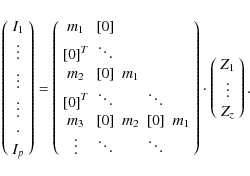
The diagonal alignment of the weighting factors is clearly evident, since they indicate the pixel at which a specific line begins to contribute to the Z-velocity grid, and how it migrates through the bins as we go through our measurement points. We note that the alignment is diagonal strictly only if the distance between two measurement points precisely equals the binsize of our velocity grid, which is not always the case. If the binsize is larger, some weighting factors are allocated one below the other, whereas for too small a binsize, they can be shifted by more than one column.
3 Optically thin versus optically thick lines
In Eq. (7), we assume that each datapoint is a linear combination of different contributions from our sought-after common line pattern. According to the Eddingtion-Barbier relation in LTE for the optically thin case, we write for the line depth (Boehm-Vitense 1989)
where
| (13) |
![\begin{figure}
\par\includegraphics[width=8.4cm,clip]{12467fg1.eps}
\end{figure}](/articles/aa/full_html/2009/45/aa12467-09/img48.png)
|
Figure 1:
Changes in the line profile with increasing
|
| Open with DEXTER | |
Thus, it seems obvious that the assumption about linearly added line profiles only holds for weak lines. For optically thick lines, where
![]() or is greater than 1, Eq. (12)
is no longer a valid approximation, since it can easily produce total
line depths >1. In general, we search for a line-summing rule
for
or is greater than 1, Eq. (12)
is no longer a valid approximation, since it can easily produce total
line depths >1. In general, we search for a line-summing rule
for
![]() that meets the following criteria:
that meets the following criteria:
- i)
-
- ii)
-
 for
for

- iii)
-
 for any R2;
 - iv)
-

- v)
-
Although this formula was derived in a totally heuristic manner, it is obvious that it is able to produce far more reliable results than a simple linear approach, especially when
as illustrated in Fig. 1. In the case of NLTE,
We instead need another formula that interpolates
![]() between Eq. (12), which is for both weak lines and the wings of strong lines, and Eq. (15), which is for the optically thick parts of the line. Introducing the quantity
between Eq. (12), which is for both weak lines and the wings of strong lines, and Eq. (15), which is for the optically thick parts of the line. Introducing the quantity
the approximation of the line profile is given by the interpolation formula according to Minnaert (1935):
For strong lines, where
We propose a new application of this formula, which has so far only
been employed to calculate equivalent widths and curves of growth.
Following our derivation given above, we state that the quantity
![]() can be regarded as the sum of different terms that contribute to the
absorption in the line, as an extreme case for instance, the sum over
the absorbing atoms. It therefore seems reasonable that the combination
of
can be regarded as the sum of different terms that contribute to the
absorption in the line, as an extreme case for instance, the sum over
the absorbing atoms. It therefore seems reasonable that the combination
of
![]() for different spectral lines is given by the sum
for different spectral lines is given by the sum
![]() of all the contributing quantities. For a blended line profile, we then write
of all the contributing quantities. For a blended line profile, we then write
To find
Combining Eqs. (18) and (19) provides a formula that enables us to calculate the line depth at a given wavelength for an arbitrary number of contributing lines, given their individual local line depths and their saturation levels. For a blended line profile, the saturation depth for each contributing line is obtained by interpolating the surfaces as shown in Fig. 2. The quantity
To calculate line profiles, we must determine in practice the source function. Only in the case of LTE
![]() is known (namely
is known (namely
![]() .
For the Milne-Eddington Model of line transfer, Mihalas (1978)
provides a formula for the saturation depth of a line that depends only
on temperature and wavelength, and neglects scattering in both the
continuum and line (assuming LTE in the line). In our case, we often
deal with strong lines that do not form in LTE and scattering is
present. This approach then seems unsatisfactory also when we take into
account that level population depends on the excitation energy of the
ground state for a given electronic transition. Therefore, to estimate
saturation depths as accurately as possible, we employed the code
STOPRO (Solanki 1987; Frutiger et al. 2000; Berdyugina et al. 2003),
solving the polarized radiative transfer equations
for 33 different elements and ions, 6 stellar
atmospheric models (Kurucz 1993), 31
wavelengths covering the region from 4000 to 10 000 Å,
and every possible lower excitation energy starting
from 0.1 eV and increasing in 0.3 eV steps (the
maximal lower excitation energy for an ion is of course lower than the
next ionization energy level).
.
For the Milne-Eddington Model of line transfer, Mihalas (1978)
provides a formula for the saturation depth of a line that depends only
on temperature and wavelength, and neglects scattering in both the
continuum and line (assuming LTE in the line). In our case, we often
deal with strong lines that do not form in LTE and scattering is
present. This approach then seems unsatisfactory also when we take into
account that level population depends on the excitation energy of the
ground state for a given electronic transition. Therefore, to estimate
saturation depths as accurately as possible, we employed the code
STOPRO (Solanki 1987; Frutiger et al. 2000; Berdyugina et al. 2003),
solving the polarized radiative transfer equations
for 33 different elements and ions, 6 stellar
atmospheric models (Kurucz 1993), 31
wavelengths covering the region from 4000 to 10 000 Å,
and every possible lower excitation energy starting
from 0.1 eV and increasing in 0.3 eV steps (the
maximal lower excitation energy for an ion is of course lower than the
next ionization energy level).
To combine all formulae together, we recall our empirical line-summing formula in Eq. (14), where we had to assume that all saturation depths equal one, and compare this with the interpolation formulae Eqs. (18) and (19). We expand Eq. (18) into a Taylor series for two lines
![]() ,
by setting
,
by setting
![]() and
and
![]() equal to 1 and obtain
equal to 1 and obtain

|
= | 
|
|
| = | ![$\displaystyle \sum_{\left\vert\alpha\right\vert}\frac{\textrm{D}^{\alpha}R_{{\r...
...{[\vec{R}=0]}}{\alpha!}\cdot\vec{R}^{\alpha}=R_1\!+\!R_2-R_1\!\cdot\!R_2+\ldots$](/articles/aa/full_html/2009/45/aa12467-09/img85.png)
|
(20) |
We can immediately see that Eq. (14) represents the first two non-zero terms of the Taylor expansion of the interpolation formula. Our estimation was therefore quite accurate, and can be helpful in practice, if saturation levels are unknown, and one benefits from the simplicity of Eq. (14).
![\begin{figure}
\par\includegraphics[width=8.8cm,clip]{12467fg2.eps}
\end{figure}](/articles/aa/full_html/2009/45/aa12467-09/img86.png)
|
Figure 2: Saturation levels for Fe I lines with lower excitation energies of 4.6 eV calculated by the code STOPRO. |
| Open with DEXTER | |
4 Numerical implementation
A common problem in spectral analysis is optimal binning. Spectral lines in the blue part of a spectrum are narrower than those at red wavelengths, since (non-transitional) broadening effects depend on wavelength. After transforming the wavelength scale into the velocity domain centered on the line wavelength, we can compare line profiles from different wavelength regions. However, any predefined velocity grid (usually at equidistant points) will never match measured data points transformed into the velocity space of a given line. The easiest way is to simply assign the measured velocity to the closest gridpoint. In such a case, however, one disregards the very accurate wavelength information of a spectrum (accurate to a fraction of an Angstrom). Here we propose to employ inverse interpolation, allowing multiple gridpoints to incorporate information of one datapoint.
We implemented quadratic inverse interpolation for NDD and the methods used for comparison, yielding a noticeable improvement in retrieved common line patterns. A detailed description is given in Appendix A, where we also present a practical algorithm for inverse spline interpolation.
Since Eqs. (14) and (18) are nonlinear functions, there is no matrix representation that would enable us to employ Eq. (5) to find a solution in Z. Thus, we have to apply iterative methods to approach a least squares solution in Z. We intentionally do not write the
solution, because we show later that, depending on how densely lines
are blended with each other, multiple minima may appear in the topology
of solutions. In Appendix B, we present two algorithms implemented to find a minimum; the Gauss-Newton with Minimization (GNwM) method and the Levenberg-Marquardt (LM) method. Although the latter is in general preferable because it minimizes the ![]() merit function far more efficiently, the former should not be underestimated because of its simplicity.
merit function far more efficiently, the former should not be underestimated because of its simplicity.
Another problem, which is atypical in the optimization of functions, is that we do not have a ``model'' function that depends on our z parameters, but rather it is the true form of our function depending on the number of parameters that is unknown. Therefore, the derivatives necessary for the Jacobi and Hessian matrices in the solving algorithms are also unknown, and need to be determined for each equation separately. Iterative evaluation of derivatives would cause our code to be extremely slow since we consider 104 equations and more, depending on as many as several hundred parameters. Therefore, we resolved this problem analytically, by determining all partial derivatives when we defined our system of nonlinear equations, depending on the number of contributing blends and the different gridpoints that they contribute to (see Appendix C). We note that these two numbers are not necessarily equal, which is the case for only two line centers lying within the velocity bin, and causes additional problems in finding the derivatives.
4.1 Critical blends
![\begin{figure}
\par\includegraphics[width=8.8cm,clip]{12467fg3.eps}
\end{figure}](/articles/aa/full_html/2009/45/aa12467-09/img88.png)
|
Figure 3:
Performance of our NDD method in recovering common line patterns from a blended line profile with line center separation
|
| Open with DEXTER | |
As we have mentioned, the ability of a deconvolution method to
identify a common line pattern in blended line profiles depends on the
proximity of the line centers. For instance, if we have dozens of lines
that are broadened significantly and separated by only fractions of an
Angstrom, they would form a broad ``valley'' with many degenerate
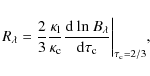
solutions for the instrinsic line profile. We approximate the Doppler
broadening of a line by
where
For a separation of
Figure 3 illustrates the ability of our deconvolving code to recover the original line profiles. We blend two identical line patterns, apply our code and compare the retrieved profile to the original single input pattern. We plot the sum of the variance (
5 Results
5.1 Atomic profiles: Stokes I
We simulated an intensity spectrum containing 7 blended spectral
lines (Fig. 4), among them two iron ions, as well as vanadium and
nickel, each with very different lower excitation energies (to test the
reliability of the Minnaert approach and its dependence on individual
saturation levels, see Eq. (18)),
to probe the functionality of both the different approaches and the
nonlinear solving methods. This does not represent a true spectrum
since the real line centers were shifted, to produce a challenging
blended profile. Therefore, the abscissa marks are omitted, both ![]() and instrumental broadening were assumed to have particular values, and we assumed a noise level of
and instrumental broadening were assumed to have particular values, and we assumed a noise level of ![]()
![]() .
The line central depths
.
The line central depths
![]() range from 0.38 to 0.66, and they were ``measured'' by simulating
single line profiles. We emphasize that the deconcolving performance
relies on precise knowledge of the parameters defining the weighting
factors mi. For Stokes I, the line central depth is the only determining parameter, and, as can be seen in Eq. (1),
if they are concordant with the (well-normalized!) spectrum, the
recovered Zeeman pattern should have normalized wings and a central
line depth dc,Z exactly equal to 1,
regardless of the strength of the original line depths. Only such a
common line pattern, scaled to individual line depths, and treated
according to Eqs. (18) and (19)
for blended profiles, will be able to reproduce the original spectrum.
Therefore, the true central line depth of the retrieved Zeeman pattern
is a strong indication of the effectiveness of a multi-line method.
range from 0.38 to 0.66, and they were ``measured'' by simulating
single line profiles. We emphasize that the deconcolving performance
relies on precise knowledge of the parameters defining the weighting
factors mi. For Stokes I, the line central depth is the only determining parameter, and, as can be seen in Eq. (1),
if they are concordant with the (well-normalized!) spectrum, the
recovered Zeeman pattern should have normalized wings and a central
line depth dc,Z exactly equal to 1,
regardless of the strength of the original line depths. Only such a
common line pattern, scaled to individual line depths, and treated
according to Eqs. (18) and (19)
for blended profiles, will be able to reproduce the original spectrum.
Therefore, the true central line depth of the retrieved Zeeman pattern
is a strong indication of the effectiveness of a multi-line method.
![\begin{figure}
\par\includegraphics[width=8.8cm,clip]{12467fg4.eps}
\end{figure}](/articles/aa/full_html/2009/45/aa12467-09/img100.png)
|
Figure 4: Simulated intensity spectrum of 7 blended lines. The dashed vertical lines mark the line centers; element names and ionization levels are labelled at the bottom. |
| Open with DEXTER | |
We applied the conventional LSD (``normal LSD''), given by Eq. (6), and the deblending, yet linear method, corresponding to Eq. (11). Both methods can be solved using Eq. (5). We compare them to our NDD method according to our realization of the Minnaert interpolation formula, applying both the Gauss-Newton with Minimization and the Levenberg-Marquardt method for the iterative solving of the nonlinear sets of equations (see Fig. 5).
``Normal LSD'' (dash-dotted curve at the bottom), which is not
a true deconvolution method, fails in this attempt, when all lines are
heavily blended, resulting in strong wiggles in the wings, a continuum
level dependent on the number of blended lines, if there is a
noticeable continuum at all, and a central line depth significantly
smaller than 1. The other linear, but deconvolution approach (dashed
line) is far more successfull, but the wings are (asymmetrically)
broadened, and the line center does not reach 0. Both of these results
infer that the linear approach for this spectrum is unsuccessfull,
because the absorbing region is entirely optically thick. When the
Minnaert formula and inverse quadratic interpolation are applied, as
presented in Sect. 4,
the result is a noticeably smoother profile compared to a ``nearest
bin'' attempt. The nonlinear (NDD) method reproduces a fairly perfect
profile within the line, showing a central line depth ![]() 1.
The differences between the two solving numerical methods are marginal,
so the two profiles almost coincide. However, in the far wings of the
Zeeman pattern, which are arguably already in the continuum, the
nonlinear solving causes errors, because of the handling of small
numbers (if we recall that we operate with 1-I). This problem should be solved by applying boundary conditions to the continuum part of the profile.
1.
The differences between the two solving numerical methods are marginal,
so the two profiles almost coincide. However, in the far wings of the
Zeeman pattern, which are arguably already in the continuum, the
nonlinear solving causes errors, because of the handling of small
numbers (if we recall that we operate with 1-I). This problem should be solved by applying boundary conditions to the continuum part of the profile.
![\begin{figure}
\par\includegraphics[width=8.8cm,clip]{12467fg5.eps}
\end{figure}](/articles/aa/full_html/2009/45/aa12467-09/img102.png)
|
Figure 5: Recovered intensity pattern from different methods employed to the atomic spectrum given in Fig. 4. |
| Open with DEXTER | |
5.2 Molecular profiles: Stokes I
In molecular bands and especially in the band head, a large number of
blends contribute to the measured line profile, and serious
deconvolution and provision for nonlinearity become mandatory. To
illustrate the capabilities of our new method, we applied the method to
a simulated molecular TiO ![]() (0, 1)
band at 7591 Å, as shown in Fig. 6.
Our NDD technique recovers a common line pattern that almost coincides
with the input Z-profile except for the right wing of the line. This is
due to the band head, where the bulk of blends interfere with each
other in a way that basically removes the individual profiles,
precluding a unique solution. As mentioned before, this problem
increases for greater broadening and more significant blending.
Nevertheless, our method is
capable of retrieving the necessary details of the line profile (e.g.,
width, see Fig. 7), which features a line central depth of virtually
equal 1, and being easily able to identify possible irregularities
within the entire profile. A comparison with the results for the linear
attempt shows that the effects of nonlinearity become noticeable in
terms of their conspicuously asymmetric wings and shallow central
profile. Again, ``normal LSD'' fails, because it lacks deconvolving
ability.
(0, 1)
band at 7591 Å, as shown in Fig. 6.
Our NDD technique recovers a common line pattern that almost coincides
with the input Z-profile except for the right wing of the line. This is
due to the band head, where the bulk of blends interfere with each
other in a way that basically removes the individual profiles,
precluding a unique solution. As mentioned before, this problem
increases for greater broadening and more significant blending.
Nevertheless, our method is
capable of retrieving the necessary details of the line profile (e.g.,
width, see Fig. 7), which features a line central depth of virtually
equal 1, and being easily able to identify possible irregularities
within the entire profile. A comparison with the results for the linear
attempt shows that the effects of nonlinearity become noticeable in
terms of their conspicuously asymmetric wings and shallow central
profile. Again, ``normal LSD'' fails, because it lacks deconvolving
ability.
![\begin{figure}
\par\includegraphics[width=8.8cm,clip]{12467fg6.eps}
\end{figure}](/articles/aa/full_html/2009/45/aa12467-09/img104.png)
|
Figure 6:
Simulated molecular TiO |
| Open with DEXTER | |
![\begin{figure}
\par\includegraphics[width=8.8cm,clip]{12467fg7.eps}
\end{figure}](/articles/aa/full_html/2009/45/aa12467-09/img105.png)
|
Figure 7: Recovered intensity pattern from different methods employed to study the molecular band given in Fig. 6. |
| Open with DEXTER | |
6 Conclusion
Our nonlinear approach to deconvolving blended line profiles by applying the Minneart interpolation formula, combined with the advantages provided by inverse interpolation, represents a significant revision of least squares deconvolution techniques, mainly because the latter do not incorporate a deconvolution of blended lines. Given a linemask that includes all relevant atomic or molecular data, we are able to disentangle arbitrarily heavily blended spectra in a physically consistent manner, fully abandoning any preliminary assumptions about the intrinsic single line profile, apart from its existence. This allows us to retrieve the true common line patterns even from a limited number of blended lines and will enable (Zeeman) Doppler Imaging to be applied even to noisy datasets of narrow spectral intervals.
Our method is also able to properly disentangle molecular bands consisting of many tens of blended line profiles within a narrow spectral range. Heavily broadened molecular spectra do not offer, however, a unique solution for the recovery of an intrinsic line profile: results always show depressed right wings. For the time being, it is nonetheless the tool most capable of identifying weak features in molecular absorption lines.
We place emphasis on the importance of a proper deconvolution of the spectrum to be analyzed, highlighting the need to disentangle blends. As shown in the derived common line patterns in Sect. 5, any non-deconvolving method imposes additional line broadening by neglecting the influence of close-by blends. In a forthcoming paper, we discuss whether ZDI codes based on these methods infer stellar spots at systematically higher lattitudes, due to a technical artifact.
The method described in the present paper offers a general and direct formalism concerning how spectral line parameters, as well as ambient and instrumental effects affect an observed intensity profile. It can be used to address a variety of problems in stellar spectrum analysis, and it is likely that it will find more general applications in many types of spectroscopy, where the quality of data is insufficient to apply direct fitting of spectra.
AcknowledgementsThis work is supported by the EURYI (European Young Investigator) Award provided by the European Science Foundation (see www.esf.org/euryi http://www.esf.org/euryi) and SNF grant PE002-104552.
Appendix A: Inverse interpolation
Each datapoint in a spectrum has a distinct distance in wavelength to the center of line
![]() for the spectral line i, which in turn corresponds to a distance in velocity space
for the spectral line i, which in turn corresponds to a distance in velocity space
![]() .
The grid for which we wish to retrieve our common line pattern Z consists of equidistant points, in other words, bins of constant binsize
.
The grid for which we wish to retrieve our common line pattern Z consists of equidistant points, in other words, bins of constant binsize
![]() .
If we consider
.
If we consider
![]() km s-1 and a pixel with
km s-1 and a pixel with
![]() km s-1, one is willing to argue that it corresonds to the gridpoint
km s-1, one is willing to argue that it corresonds to the gridpoint
![]() ,
simply because it is the closest one. However, one could instead
inversely interpolate, so as to express the datapoint in terms of
multiple Z-gridpoints. Applying quadratic interpolation, we obtain
,
simply because it is the closest one. However, one could instead
inversely interpolate, so as to express the datapoint in terms of
multiple Z-gridpoints. Applying quadratic interpolation, we obtain
| (A.1) |
where the constants p0,p1,p2 can be calculated with the Lagrange-formula for interpolation:
|
(A.2) |
yielding
| (A.3) |
Another method that was implemented was that of spline interpolation, since we expect our Zeeman pattern to be smooth and continuous. The difficulty lies in analytically solving the linear system of equations with its typical tridiagonal, strictly diagonally dominant
and
After Gauss elimination, Eq. (A.4) can be written as
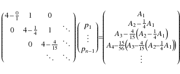
To express the coefficients pi after back-substitution of this linear system of equations, we introduce the recursive sequences
Using this, we can write for pi,
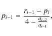
or, without the use of the ri's:
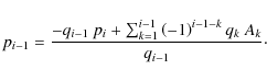
|
(A.10) |
We have presented the sought-after coefficients in Eq. (A.5) in terms of the quantities Ai, where the Ai's in turn are linearly dependent on Zi, as given in Eq. (A.4). Even if a datapoint is affected by only one spectral line, it will then be represented as a linear combination of all elements of Z, where in the case of quadratic interpolation, it will always be represented by three of them.
Appendix B: Solving algorithms
For the Gauss-Newton method, following Nipp (2002), we represent our set of equations by

where yi are the measurement values and ri the residuals. We search for a
where
where

|
(B.4) |
After k iterations, we then force Zk to converge and assume that
The Levenberg-Marquardt method is more efficient, because of its favorable direction of descent. Again, we define the ![]() merit function in terms of least squares to be
merit function in terms of least squares to be
![\begin{displaymath}
\chi^2\!\left(\mathbf{Z}\right)=\sum_{i=1}^p\left[\frac{y_i-f_i\!\left(\mathbf{Z}\right)}{\sigma_i}\right]^2\cdot
\end{displaymath}](/articles/aa/full_html/2009/45/aa12467-09/img141.png)
Sufficiently close to the minimum, we expect the ![]() function to be well approximated by a quadratic form, according to Press (1992)
function to be well approximated by a quadratic form, according to Press (1992)
where ![]() is an z-vector and
D is an
is an z-vector and
D is an ![]() matrix. If Eq. (B.6) is a good approximation, then one leap will take us from the current values
matrix. If Eq. (B.6) is a good approximation, then one leap will take us from the current values
![]() to the minimizing ones
to the minimizing ones
![]() ,
i.e.,
,
i.e.,
![\begin{displaymath}
\mathbf{Z}_{\rm min}=\mathbf{Z}_{\rm cur}+\mathbf{D}^{-1}\cdot\left[-\nabla\chi^2\!\left(\mathbf{Z}_{\rm cur}\right)\right].
\end{displaymath}](/articles/aa/full_html/2009/45/aa12467-09/img147.png)
However, if (B.6) does not represent the shape of ![]() at
at
![]() ,
i.e., when we are far from the minimum, then all we can do is apply the
steepest descent method, as we did for the Gauss-Newton minimization
,
i.e., when we are far from the minimum, then all we can do is apply the
steepest descent method, as we did for the Gauss-Newton minimization
The Levenberg-Marquardt method adopts both extremes, by varying smoothly between the inverse-Hessian method (B.7) and the steepest descent method (B.8), depending on how far we are from the minimum. In addition, it provides an estimated covariance matrix of the standard errors in the fitted values Z.
Appendix C: Derivative of the extended interpolation formula
For our solving algorithms, we develop the partial derivatives for each
equation with respect to each element of our sought-after common line
pattern
![]() to produce the Jacobi matrix and the Hessian matrix, which can also be approximated by the first derivatives. If we define
to produce the Jacobi matrix and the Hessian matrix, which can also be approximated by the first derivatives. If we define
![]() for
for
![]() ,
where z is the number of parameters in Z, and
,
where z is the number of parameters in Z, and
![]() ,
then
we rewrite Eq. (19) with the weights mj as
,
then
we rewrite Eq. (19) with the weights mj as
and Eq. (18), for
![\begin{displaymath}
f_i=\frac{s_i}{1+d_{{\rm tot}}s_i},\quad\textrm{with}\quad s_i=\sum_{j\in\left[j\right]_i}X_j
\end{displaymath}](/articles/aa/full_html/2009/45/aa12467-09/img155.png)
where
Therefore, for the elements of the Jacobi matrix
References
- Berdyugina, S. V., Solanki, S. K., & Frutiger, C. 2003, A&A, 412, 513 [NASA ADS] [CrossRef] [EDP Sciences]
- Boehm-Vitense, E. 1989, Introduction to stellar astrophysics (New York: Cambridge University Press)
- Donati, J. F., Semel, M., Carter, B. D., Rees, D. E., & Cameron, A. C. 1997, 291, 658
- Frutiger, C., Solanki, S. K., Fligge, M., & Bruls, J. H. M. J. 2000, A&A, 358, 1109 [NASA ADS]
- Kurucz, R. L. 1993, CDROM No. 13
- Martínez Gonzáles, M. J., Asensio Ramos, A., Carroll, T. A., et al. 2008, 486, 637
- Mihalas, D. 1978, Stellar atmospheres (San Francisco: W. H. Freeman and Company)
- Minnaert, M. 1935, 10, 40
- Nipp, K. 2002, Lineare Algebra (Zurich: vdf)
- Press, W. H. 1992, Numerical Recipes (New York: Cambridge University Press)
- Semel, M. 1989, 225, 456
- Semel, M., & Li, J. 1996, Sol. Phys., 164, 417 [NASA ADS] [CrossRef]
- Solanki, S. K. 1987, Ph.D. Thesis, ETH, Zurich, Switzerland
- Unsoeld, A. 1968, Physik der Sternatmosphaeren (Berlin: Springer-Verlag)
All Figures
|
|
Figure 1:
Changes in the line profile with increasing
|
| Open with DEXTER | |
| In the text | |
|
|
Figure 2: Saturation levels for Fe I lines with lower excitation energies of 4.6 eV calculated by the code STOPRO. |
| Open with DEXTER | |
| In the text | |
|
|
Figure 3:
Performance of our NDD method in recovering common line patterns from a blended line profile with line center separation
|
| Open with DEXTER | |
| In the text | |
|
|
Figure 4: Simulated intensity spectrum of 7 blended lines. The dashed vertical lines mark the line centers; element names and ionization levels are labelled at the bottom. |
| Open with DEXTER | |
| In the text | |
|
|
Figure 5: Recovered intensity pattern from different methods employed to the atomic spectrum given in Fig. 4. |
| Open with DEXTER | |
| In the text | |
|
|
Figure 6:
Simulated molecular TiO |
| Open with DEXTER | |
| In the text | |
|
|
Figure 7: Recovered intensity pattern from different methods employed to study the molecular band given in Fig. 6. |
| Open with DEXTER | |
| In the text | |
Copyright ESO 2009
Current usage metrics show cumulative count of Article Views (full-text article views including HTML views, PDF and ePub downloads, according to the available data) and Abstracts Views on Vision4Press platform.
Data correspond to usage on the plateform after 2015. The current usage metrics is available 48-96 hours after online publication and is updated daily on week days.
Initial download of the metrics may take a while.