| Issue |
A&A
Volume 507, Number 3, December I 2009
|
|
|---|---|---|
| Page(s) | 1763 - 1784 | |
| Section | Catalogs and data | |
| DOI | https://doi.org/10.1051/0004-6361/200912382 | |
| Published online | 08 October 2009 | |
A&A 507, 1763-1784 (2009)
The Nainital-Cape Survey
III. A search for pulsational variability in chemically peculiar stars
S. Joshi1 - D. L. Mary2 - N. K. Chakradhari3 - S. K. Tiwari1 - C. Billaud2
1 - Aryabhatta Research Institute of Observational Sciences (ARIES), Manora Peak, Nainital, India
2 -
Université de Nice Sophia Antipolis, Observatoire de la Côte d'Azur, Nice, France
3 -
School of Studies in Physics and Astrophysics, Pt. Ravishankar Shukla University, Raipur, India
Received 24 April 2009 / Accepted 2 September 2009
Abstract
Context. The Nainital-Cape survey is a dedicated research
programme to search for and study the pulsational variability in
chemically peculiar stars in the Northern Hemisphere.
Aims. The aim of the survey is to search for such chemically peculiar stars that are pulsationally unstable.
Methods. The observations of the sample stars were carried out
in high-speed photometric mode using a three-channel fast photometer
attached to the 1.04-m Sampurnanand telescope at ARIES.
Results. The new photometric observations confirmed that the
pulsational period of star HD 25515 is 2.78-hrs. The repeated
time-series observations of HD 113878 and HD 118660 revealed
that previously known frequencies are indeed present in the new data
sets. We have estimated the distances, absolute magnitudes, effective
temperatures and luminosities of these stars. Their positions in the
H-R diagram indicate that HD 25515 and HD 118660 lie near the
main-sequence while HD 113878 is an evolved star. We also present
a catalogue of 61 stars classified as null results, along with the
corresponding 87 frequency spectra taken from 2002-2008. A statistical
analysis of these null results shows, by comparison with past data,
that the power of the noise in the light curves has slightly increased
during the last few years.
Key words: stars: chemically peculiar - stars: oscillations - stars: variables: ![]() Sct
Sct
1 Introduction
A survey project, the ``Nainital-Cape Survey'' was initiated in 1997 between the Aryabhatta Research Institute of Observational Sciences (ARIES), Nainital, and the South African Astronomical Observatory (SAAO), Capetown, to search for and study the pulsational variability in chemically peculiar (CP) A-F stars. The atmospheres of these stars have an inhomogeneous distribution of chemical elements which are frequently seen as abundance spots on stellar surfaces and as clouds of chemical elements concentrated at certain depths along the stellar radius (see, for example, Kochukhov et al. 2004a; Lueftinger et al. 2003; Ryabchikova et al. 2006, 2005, 2002). The inhomogeneity with high abundance gradients is explained by microscopic radiative diffusion processes depending on the balance between gravitational pull and uplift by the radiation field through absorption in spectral lines (Michaud 1970; Michaud et al. 1981; Leblanc et al. 2009). Therefore, the CP stars are excellent test objects for astrophysical processes like diffusion, convection, and stratification in stellar atmospheres in the presence of rather strong magnetic fields.A class of CP (CP2) stars known as Ap (A-peculiar) stars, which
rotate considerably more slowly than spectroscopically normal main
sequence stars have similar effective temperatures, strong magnetic
fields, normal or below-solar concentrations of light and iron-peak
elements, and overabundances of rare Earth elements. A fraction of cool
Ap stars in the effective temperature range of ![]() 6400 to 8100 K (Kochukhov & Bagnulo 2006)
exhibit anomalously strong Sr, Cr and Eu lines coupled with
high-magnetic fields from a few to as high as 24.5 kGauss (Kurtz
et al. 2006b). Those stars which pulsate in the period of
range 5.65 to 22-min (Kreidl 1985; Kochukhov 2008), with photometric amplitude variations of less than 10 milli-magnitude (mmag) in the Johnson B filter, and spectroscopic radial velocity variations of 0.05 to 5-km s-1, are known as rapidly oscillating Ap (roAp) stars. The roAp pulsations are attributed to low-order (l< 3), high-overtone (
6400 to 8100 K (Kochukhov & Bagnulo 2006)
exhibit anomalously strong Sr, Cr and Eu lines coupled with
high-magnetic fields from a few to as high as 24.5 kGauss (Kurtz
et al. 2006b). Those stars which pulsate in the period of
range 5.65 to 22-min (Kreidl 1985; Kochukhov 2008), with photometric amplitude variations of less than 10 milli-magnitude (mmag) in the Johnson B filter, and spectroscopic radial velocity variations of 0.05 to 5-km s-1, are known as rapidly oscillating Ap (roAp) stars. The roAp pulsations are attributed to low-order (l< 3), high-overtone (![]() ), non-radial p-modes and are classically explained by the oblique pulsator model (Kurtz 1982).
This model supposes that the pulsation axis is aligned to the magnetic
axis which is oblique to the rotation axis. As the star rotates, the
variations in the pulsational amplitude can be observed by a distant
observer. Recent theoretical studies of roAp stars show that the axis
of the p-mode pulsations is not exactly aligned with the magnetic field because of the centrifugal force (Bigot & Dziembowski 2002). Excitation of pulsations in roAp stars is governed by the
), non-radial p-modes and are classically explained by the oblique pulsator model (Kurtz 1982).
This model supposes that the pulsation axis is aligned to the magnetic
axis which is oblique to the rotation axis. As the star rotates, the
variations in the pulsational amplitude can be observed by a distant
observer. Recent theoretical studies of roAp stars show that the axis
of the p-mode pulsations is not exactly aligned with the magnetic field because of the centrifugal force (Bigot & Dziembowski 2002). Excitation of pulsations in roAp stars is governed by the ![]() -mechanism acting in the
H I
ionization zone, with the additional influence of the magnetic
quenching of convection and composition gradients built up by the
atomic diffusion (Balmoforth et al. 2001; Cunha 2002; Vauclair & Théado 2004).
These magneto-acoustic pulsators provide a unique opportunity to study
pulsations in the presence of chemical inhomogeneities and strong
magnetic fields.
-mechanism acting in the
H I
ionization zone, with the additional influence of the magnetic
quenching of convection and composition gradients built up by the
atomic diffusion (Balmoforth et al. 2001; Cunha 2002; Vauclair & Théado 2004).
These magneto-acoustic pulsators provide a unique opportunity to study
pulsations in the presence of chemical inhomogeneities and strong
magnetic fields.
Apart from the roAp stars, another class of CP stars (CP1) known as Am
(A-metallic) stars preferably found within close binary systems,
exhibit low-rotational velocities, lack of magnetic fields, apparent
underabundance of calcium and scandium, and has overabundance of
Fe-peak elements. The former near exclusion between pulsational
variability and Am-type chemical peculiarity has evolved considerably
in recent years, and this dichotomy is no longer clear-cut. Indeed,
pulsations of the ![]() -Scuti type
-Scuti type![]() have been seen in many Am stars (e.g. Kurtz 1989; Martinez et al. 1999; Kurtz & Martinez 2000; Joshi et al. 2003; González et al. 2008),
but our understanding of the physics of pulsating Am stars is still far
from being complete. Theoretical models can for instance partially
explain that evolved Am stars can pulsate (
have been seen in many Am stars (e.g. Kurtz 1989; Martinez et al. 1999; Kurtz & Martinez 2000; Joshi et al. 2003; González et al. 2008),
but our understanding of the physics of pulsating Am stars is still far
from being complete. Theoretical models can for instance partially
explain that evolved Am stars can pulsate (![]() -mechanism in He II can drive the pulsations in evolved Am stars) and that marginal Am stars can be low-amplitude
-mechanism in He II can drive the pulsations in evolved Am stars) and that marginal Am stars can be low-amplitude ![]() -Scuti
stars (a sufficient amount of He remains to drive low-amplitude
oscillations). However, less well understood are the mechanisms of
pulsations in classical Am stars (Kurtz & Martinez 2000),
-Scuti
stars (a sufficient amount of He remains to drive low-amplitude
oscillations). However, less well understood are the mechanisms of
pulsations in classical Am stars (Kurtz & Martinez 2000), ![]() -Scuti type pulsations in Ap stars (González et al. 2008), the origin of the abundance anomalies either from a superficial or from a much deeper mixing zone (Leblanc & Alecian 2008; Leblanc et al. 2009), the co-existence of
-Scuti type pulsations in Ap stars (González et al. 2008), the origin of the abundance anomalies either from a superficial or from a much deeper mixing zone (Leblanc & Alecian 2008; Leblanc et al. 2009), the co-existence of ![]() -Scuti and
-Scuti and ![]() -Doradus type pulsations in Am stars (King et al. 2006; Henry & Fekel 2005), limits where chemical peculiarity and pulsations can coexist and where they are mutually exclusive (Hekker et al. 2008) and possible excitation of solar like oscillations in Am stars (Carrier et al. 2007).
-Doradus type pulsations in Am stars (King et al. 2006; Henry & Fekel 2005), limits where chemical peculiarity and pulsations can coexist and where they are mutually exclusive (Hekker et al. 2008) and possible excitation of solar like oscillations in Am stars (Carrier et al. 2007).
The rich pulsation spectra of roAp and pulsating Am stars not only helps us to study the interaction of pulsations and chemical peculiarities but also several important astrophysical parameters such as mass, luminosity, rotational period or magnetic field strength can also be inferred, or at least constrained (Balmforth et al. 2001; Cunha 2002; Saio 2005; Bruntt et al. 2009).
However, despite several searches (e.g. Nelson & Kreidl 1993; Martinez & Kurtz 1994; Handler & Paunzen 1999; Martinez et al. 2001; Dorokhova & Dorokhov 2005; Joshi et al. 2006) only about 40 roAp stars are known to date (Kochukhov 2008).
This dearth of roAp stars demands high-precision systematic
surveys. In this context, the ``Nainital-Cape'' survey is an effort to
search for pulsational variability in Ap and Am stars. In the last
decade, several results have been obtained from this survey. They are
summarized in Table 1: HD 12098 was discovered as a roAp star (Girish et al. 2001), and pulsations of the ![]() -Scuti type were discovered in 6 CP stars : HD 13038, HD 13079 (Martinez et al. 2001), HD 98851, HD 102480 (Joshi et al. 2003), HD 113878 and HD 118660 (Joshi et al. 2006).
HD 98851 and HD 102480 are unusual pulsators in the sense
they exhibit alternating high and low maxima (i.e., the amplitude of
the pulsations is high and low in a cyclic way).
-Scuti type were discovered in 6 CP stars : HD 13038, HD 13079 (Martinez et al. 2001), HD 98851, HD 102480 (Joshi et al. 2003), HD 113878 and HD 118660 (Joshi et al. 2006).
HD 98851 and HD 102480 are unusual pulsators in the sense
they exhibit alternating high and low maxima (i.e., the amplitude of
the pulsations is high and low in a cyclic way).
Table 1: Pulsating variables discovered during the ``Nainital-Cape survey''.
Since the 1980 s, the high-speed photometric technique is has been
used to search for and study the photometric light variations in short
period (![]() min)
pulsating variables. In parallel, high-resolution spectroscopic
techniques have been recently used to measure the corresponding radial
velocity (RV) variations and yielded many interesting results (e.g.
Kochukhov & Ryabchikova 2001; Mkrtichian et al. 2003; Hatzes & Mkrtichian 2004; Elkin et al. 2005; Kurtz et al. 2006a; Ryabchikova et al. 2007; Kochukhov et al. 2008; González et al. 2008).
The RV measurements are a very useful technique towards the derivation
of horizontal information obtained from the line profile variability.
Vertical information is extracted from the differential analysis of
both the amplitude and phase of spectral lines formed at different
atmospheric heights. Also, the phase information of individual spectral
lines and oscillation modes is an important tool to constrain the
chemical stratification and the physical models of the atmosphere. For
these reasons, RV studies of individual lines provide a very
powerful tool towards an atmospheric tomography of roAp stars.
min)
pulsating variables. In parallel, high-resolution spectroscopic
techniques have been recently used to measure the corresponding radial
velocity (RV) variations and yielded many interesting results (e.g.
Kochukhov & Ryabchikova 2001; Mkrtichian et al. 2003; Hatzes & Mkrtichian 2004; Elkin et al. 2005; Kurtz et al. 2006a; Ryabchikova et al. 2007; Kochukhov et al. 2008; González et al. 2008).
The RV measurements are a very useful technique towards the derivation
of horizontal information obtained from the line profile variability.
Vertical information is extracted from the differential analysis of
both the amplitude and phase of spectral lines formed at different
atmospheric heights. Also, the phase information of individual spectral
lines and oscillation modes is an important tool to constrain the
chemical stratification and the physical models of the atmosphere. For
these reasons, RV studies of individual lines provide a very
powerful tool towards an atmospheric tomography of roAp stars.
If spectroscopic studies are such an efficient tool, why continue doing photometric surveys? Despite the improved sensitivity of the high-resolution spectroscopic monitoring for searching low-amplitude oscillations in roAp candidates, the major drawback of this technique remains the small amount of observing time available at large telescopes. Traditional photometric surveys are performed on small telescopes, and are consequently relatively cheap (both in cost and telescope time). For instance, Kurtz discovered the first roAp star HD 101065 by means of high-speed photometry using the 50-cm telescope of SAAO (Kurtz 1978). Indeed, this argument in favor of photometry assumes that the photometric instruments are periodically upgraded: since the 1970 s, most or all bright stars that are observable with good signal to noise ratios using small telescopes and traditional detectors have been checked for pulsation at the mmag level. In order to push our investigations towards fainter objects, the technology of photometric surveys must consequently be updated with state-of-the-art instruments. This is one reason why ARIES decided to give a new boost to the survey by installing bigger telescopes at a better astronomical site (see Sect. 5.2, and Sagar et al. 2000; Stalin et al. 2001).
This paper is the third of a series (Paper I: Martinez et al. 2001, Paper II: Joshi et al. 2006). It is organized as follows: the selection criteria are briefly described in Sect. 2 and the techniques of observation and data analysis are described in Sect. 3. Results from the new observations of HD 25515, HD 113878 and HD 118660, along with some astrophysical parameters of these stars are presented in Sect. 4. Section 5 presents the null results and their analysis. Some conclusions are drawn in Sect. 6.
2 Selection of the candidates
To date, there are no firmly established selection criteria to maximize
the chances of detecting new variables.
Therefore our primary criterion was to choose candidates presenting
Strömgren photometric indices similar to those Ap and Am stars that
exhibit pulsational variability (Hauck & Mermilliod 1998). For this, the following range of Strömgren photometric indices was used to select the samples:
![]() ;
;
![]() ;
;
![]() ;
;
![]() ;
;
![]() and
and
![]() ,
where c1 is the Balmer discontinuity parameter (luminosity indicator), m1 is the line-blanketing parameter (metallicity indicator),
,
where c1 is the Balmer discontinuity parameter (luminosity indicator), m1 is the line-blanketing parameter (metallicity indicator), ![]() is the H
is the H![]() line strength index (indicator of temperature in the spectral range A3 to F2 and reasonably free from reddening) and b-y is also an indicator of temperature but affected by reddening. A more negative value of
line strength index (indicator of temperature in the spectral range A3 to F2 and reasonably free from reddening) and b-y is also an indicator of temperature but affected by reddening. A more negative value of
![]() [m1(standard)-m1(observed)] and
[m1(standard)-m1(observed)] and
![]() [c1(observed)-c1(standard)] means that the star is more peculiar (Crawford 1975, 1979). However, we have slightly extended (by
[c1(observed)-c1(standard)] means that the star is more peculiar (Crawford 1975, 1979). However, we have slightly extended (by ![]() 10%)
the corresponding range of indices to include the evolved and cooler
stars, hence there are sample stars not falling in the range of
Strömgren photometric indices mentioned above. The candidates were also
selected from the general catalogue of Ap and Am stars
(Renson et al. 1991) and the fifth Michigan catalogue (Houk & Swift 1999).
The roAp stars are magnetic and of the SrCrEu type, and pulsating Am
stars are non-magnetic. Since both belong to the spectral class of late
A to early F, samples were also selected from the Kudryavtsev
et al. (2006); Bychkov et al. (2003) and Høg et al. (2000).
10%)
the corresponding range of indices to include the evolved and cooler
stars, hence there are sample stars not falling in the range of
Strömgren photometric indices mentioned above. The candidates were also
selected from the general catalogue of Ap and Am stars
(Renson et al. 1991) and the fifth Michigan catalogue (Houk & Swift 1999).
The roAp stars are magnetic and of the SrCrEu type, and pulsating Am
stars are non-magnetic. Since both belong to the spectral class of late
A to early F, samples were also selected from the Kudryavtsev
et al. (2006); Bychkov et al. (2003) and Høg et al. (2000).
3 Observations and data analysis
The time-series photometric data consist of continuous 10-s integrations obtained through a Johnson B-filter. An aperture of 30
![]() was used to minimize flux variations caused by seeing fluctuations and
guiding errors. The data reduction process comprises visual inspection
of the light curve to identify and remove the bad data points,
correction for coincident counting losses, subtraction of the
interpolated sky background and correction for the mean atmospheric
extinction. After applying these corrections, the times of the
mid-points of each data sample are converted into heliocentric Julian
dates (HJD) with an accuracy of 10-5 day
(
was used to minimize flux variations caused by seeing fluctuations and
guiding errors. The data reduction process comprises visual inspection
of the light curve to identify and remove the bad data points,
correction for coincident counting losses, subtraction of the
interpolated sky background and correction for the mean atmospheric
extinction. After applying these corrections, the times of the
mid-points of each data sample are converted into heliocentric Julian
dates (HJD) with an accuracy of 10-5 day
(![]() 1 s). The reduced data comprise a time-series of HJD and B-magnitude with respect to the mean of the light curve.
1 s). The reduced data comprise a time-series of HJD and B-magnitude with respect to the mean of the light curve.
To search for periodic signals, the time-series data were classically
analyzed using a fast algorithm based on Deeming's discrete Fourier
transform (DFT) for unequally spaced data (Deeming 1975). The first step of the analysis is to inspect the DFTs of each individual light curve where the dominant frequency f1
is identified. To identify other frequencies present in the data, a
sinusoid corresponding to the dominant frequency, amplitude and phase
(of the form
![]() is subtracted from the time-series. The residuals of this fit are then
used to compute the DFT again, the resulting dominant frequency is
identified as f2
and so on. This prewhitening procedure was repeated until the residuals
were judged to be at the noise level. To search for additional
frequencies and to define the known frequencies in a better way, we
also computed the DFTs of the combined data sets for each star. We
comment further on the data analysis in the next section.
is subtracted from the time-series. The residuals of this fit are then
used to compute the DFT again, the resulting dominant frequency is
identified as f2
and so on. This prewhitening procedure was repeated until the residuals
were judged to be at the noise level. To search for additional
frequencies and to define the known frequencies in a better way, we
also computed the DFTs of the combined data sets for each star. We
comment further on the data analysis in the next section.
4 New fast photometric observations of HD 25515, HD 113878 and HD 118660
The following subsections describe the results from the follow-up observations and discuss some of the fundamental astrophysical parameters of the individual stars.4.1 HD 25515
The Strömgren indices of HD 25515 are b-y = 0.262, m1 = 0.177, c1 = 0.745 and![\begin{figure}
\par\hbox {
\includegraphics[width=9cm,height=7cm]{19353fg01.ps}\includegraphics[width=9cm,height=7cm]{19353fg02.ps} }\end{figure}](/articles/aa/full_html/2009/45/aa12382-09/img21.png)
|
Figure 1: Four typical light curves ( left) and their corresponding amplitude spectra ( right) of HD 25515 obtained in four different observing seasons. |
| Open with DEXTER | |
Table 2: Journal of fast photometric observations of HD 25515.
![\begin{figure}
\par\hbox {\includegraphics[width=9cm,height=7cm]{19353fg03.ps}\includegraphics[width=9cm,height=7cm]{19353fg04.ps} }\end{figure}](/articles/aa/full_html/2009/45/aa12382-09/img25.png)
|
Figure 2: Four typical curves ( left) and corresponding amplitude spectra ( right) of HD 113878 obtained in four different observing seasons. |
| Open with DEXTER | |
![\begin{figure}
\par\hbox {\includegraphics[width=9cm,height=5cm,clip]{19353fg05.ps}\includegraphics[width=9cm,height=5cm,clip]{19353fg06.ps} }\end{figure}](/articles/aa/full_html/2009/45/aa12382-09/img26.png)
|
Figure 3: Two typical curves ( left) and corresponding amplitude spectra ( right) of star HD 118660 obtained in two different seasons. |
| Open with DEXTER | |
Table 2 gives the
complete journal of the photometric observations. The data sets marked
with asterisks are used for frequency analysis to search for the
additional frequencies and define the known frequencies in a better way
(same asterisks convention for the next two tables).
Columns 5 and 6 of this table list the prominent frequencies
and the corresponding amplitudes, respectively. A frequency analysis of
the longest time-series (Dec. 20, 2007) shows a pulsational period
of 2.78-h (
![]() mHz). Another prominent frequency
mHz). Another prominent frequency
![]() mHz
is also visible in some amplitude spectra; however, it lies in the
region where the sky transparency has a high power, further follow-up
observations are therefore needed to strengthen the detection of this
frequency.
mHz
is also visible in some amplitude spectra; however, it lies in the
region where the sky transparency has a high power, further follow-up
observations are therefore needed to strengthen the detection of this
frequency.
Table 3: Journal of fast photometric observations of HD 113878.
Table 4: Journal of fast photometric observations of HD 118660.
4.2 HD 113878
HD 113878 was discovered as a4.3 HD 118660
The discovery of pulsations in HD 118660 was also reported by Joshi et al. (2006); it was speculated that the star might be a multi-periodic pulsating variable. To confirm this periodicity and search for additional periods, follow-up observations were carried out between 2005 and 2007. A total of 41.22 h high-speed photometric data was acquired on 11 nights. Table 4 gives the journal of the observations. The left panel of Fig. 3 shows two typical light curves obtained in two observing seasons and the corresponding amplitude spectra are shown in the right panel. The frequencies f1=0.28 and f2=0.11 mHz reported by Joshi et al. (2006) are indeed present in almost all the runs, so these new observations confirm the previously known frequencies.
4.4 Frequency analysis of the combined data
We combined the time-series data sets of HD 25515, HD 113878 and HD 118660 (marked with asterisks in Tables 2, 3 and 4) to identify the known frequencies and to search for additional frequencies. In order to obtain a good S/N ratio in the amplitude spectra, we excluded the data sets that are contaminated by large sky transparency variation and/or have a duration of less than one cycle. The amplitude spectra of these combined data set of HD 25515, HD 113878 and HD 118660 are shown in Figs. 4-6, respectively. All these Fourier transforms (FTs) are ``raw'' transforms in the sense that no low-frequency filtering to remove sky transparency fluctuations was applied to the data, other than a correction for mean extinction. The top panel of these figures are the FTs of the whole data sets mentioned in the caption of each figure while the lower panels are the FTs after successive prewhitening by f1, f2, f3, etc. Columns 2-4 of Table 5 lists the prominent frequencies, amplitudes and phases. Two frequencies f1=0.11 mHz and f2=0.03 mHz are clearly visible in the amplitude spectrum of HD 25515. However, the frequency f2 lies in the region of sky transparency variations and hence needs confirmation. In the case of HD 113878, the frequency f1 is present in both the combined and individual data sets and hence this frequency is firmly confirmed. The amplitude spectrum of HD 118660 clearly shows the presence of three prominent peaks at frequencies f1=0.054, f2=0.299 and f3=0.200 mHz. The frequency f1 has a low amplitude and a low frequency so it should be taken cautiously.
![\begin{figure}
\par\includegraphics[width=9cm,height=7.8cm]{19353fg07.ps}
\end{figure}](/articles/aa/full_html/2009/45/aa12382-09/img29.png)
|
Figure 4: Amplitude spectrum of HD 25515 after combining the time-series data marked with asterisks in Table 2. |
| Open with DEXTER | |
![\begin{figure}
\par\includegraphics[width=9cm,height=7.8cm]{19353fg08.ps}
\end{figure}](/articles/aa/full_html/2009/45/aa12382-09/img30.png)
|
Figure 5: Amplitude spectrum of HD 113878 after combining the time-series data marked with asterisks in Table 3. |
| Open with DEXTER | |
The frequencies identified using the DFT were fitted simultaneously to
the combined data by linear least-square fits that assumes that the
frequencies are perfectly known and adjusts the amplitudes and phases.
These amplitudes and phases, along with their errors, are listed in
Table 5,
which combines the time-series data sets marked with asterisks in Tables 2-4, respectively.
The phase ![]() corresponds to
t0=24553012.14302, 2452320.40523 and 2453426.38106
for HD 25515, HD 113878, and HD 118660, respectively.
The comparison of the amplitude and phase determined using both methods
are consistent with each
other. We caution that all the frequencies listed in Table 5 are subject to 1-day-1
cycle count ambiguities. In order to reduce these ambiguities and
eliminate them altogether a multi-site campaign is necessary. Note that
another efficient way to study the pulsational variability in
corresponds to
t0=24553012.14302, 2452320.40523 and 2453426.38106
for HD 25515, HD 113878, and HD 118660, respectively.
The comparison of the amplitude and phase determined using both methods
are consistent with each
other. We caution that all the frequencies listed in Table 5 are subject to 1-day-1
cycle count ambiguities. In order to reduce these ambiguities and
eliminate them altogether a multi-site campaign is necessary. Note that
another efficient way to study the pulsational variability in ![]() -Scuti
type variables is differential CCD photometry. This technique needs
nearby comparison stars of similar magnitude and color. HD 25515,
HD 113878 and HD 118660 are however brighter than nine
magnitudes and there are no nearby comparison stars of similar
magnitude and color; this renders the use of differential photometry
difficult in this case.
-Scuti
type variables is differential CCD photometry. This technique needs
nearby comparison stars of similar magnitude and color. HD 25515,
HD 113878 and HD 118660 are however brighter than nine
magnitudes and there are no nearby comparison stars of similar
magnitude and color; this renders the use of differential photometry
difficult in this case.
![\begin{figure}
\par\includegraphics[width=9cm,height=9cm]{19353fg09.ps}
\end{figure}](/articles/aa/full_html/2009/45/aa12382-09/img32.png)
|
Figure 6: Amplitude spectrum of HD 118660 after combining the time-series data marked with asterisks in Table 4. |
| Open with DEXTER | |
Table 5: Identification of the frequencies present in HD 25515, HD 113878 and HD 118660.
4.5 Fundamental parameters
We derived some astrophysical parameters of HD 25515, HD 113878 and HD 118660 using Hipparcos parallaxes (van Leeuwen 2007) and Simbad data base. Those are listed in Table 6. The calculated values for E(B-V) and the bolometric corrections (BC) for HD 25515, HD 113878 and HD 118660 are 0.02, 0.20, 0.06 mag and 0.026, 0.035, 0.035 mag, respectively. The effective temperatures of these stars were estimated using the grids of Moon & Dworetsky (1985) with typical errors of the order of 200 K.
The absolute magnitude Mv is calculated using the relation (Cox 1999)
| (1) |
where
The luminosity log
![]() were calculated using the relation
were calculated using the relation
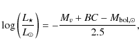
|
(2) |
where
Table 6: Astrophysical data for HD 25515, HD 113878 and HD 118660.
![\begin{figure}
\par\includegraphics[width=8.5cm,height=8.2cm,clip]{19353fg10.ps}
\end{figure}](/articles/aa/full_html/2009/45/aa12382-09/img39.png)
|
Figure 7:
An HR diagram showing the positions of HD 25515 (cross),
HD 113878 (triangle) and HD 118660 (square) in relation to
the borders of the instability strip. For the comparison evolutionary
tracks of 1.6 to 2.9 |
| Open with DEXTER | |
![\begin{figure}
\par\includegraphics[width=8.5cm,height=6.7cm,clip]{19353fg11.eps}
\end{figure}](/articles/aa/full_html/2009/45/aa12382-09/img40.png)
|
Figure 8: Statistics of the 87 runs acquired from the Nainital-Cape survey in 2002-2008. Top: distribution of the number of runs per star. Most of the stars have been observed only once. A few of them, where some variability was suspected, were observed many times. Bottom: distribution of the total time dedicated to observe one star (in hours). Most of the stars have been observed for less than 2 h (the mean is 1.6 h and the median 1.5 h). |
| Open with DEXTER | |
![\begin{figure}
\par\includegraphics[width=9cm,height=7cm,clip]{19353fg12.eps}
\end{figure}](/articles/aa/full_html/2009/45/aa12382-09/img41.png)
|
Figure 9: Distribution of the amplitude of the tallest peaks in the prewhitened spectra for the 1999-2002 data ( top) and 2002-2008 data ( bottom). |
| Open with DEXTER | |
![\begin{figure}
\par\includegraphics[width=9cm,height=7cm,clip]{19353fg13.eps}
\end{figure}](/articles/aa/full_html/2009/45/aa12382-09/img42.png)
|
Figure 10: Distribution of the positions of the tallest peaks in the prewhitened spectra for the 1999-2002 data ( top) and 2002-2008 data ( bottom). |
| Open with DEXTER | |
Table 7: Sample of stars classified as null results.
The estimated positions of HD 25515, HD 113878 and HD 118660 in the H-R diagram are shown in Fig. 7. For comparison, evolutionary tracks![]() of masses ranging from 1.6 to
2.9
of masses ranging from 1.6 to
2.9 ![]() are also over-plotted (Christensen-Dalsgaard 1993).
These models are computed with the Aarhus evolution code (ASTEC),
superior in terms of numerical precision and used extensively (Cunha 2002; Freyhammer et al. 2008a,b). For the model calculations, used compositions are
X = 0.692827 and Z = 0.02, the equation of state from Eggleton et al. (1973),
opacities from OPAL92, and the convection was treated with
mixing-length theory. No convective-core overshoot, diffusion and
settling was considered to compute these models (Christensen-Dalsgaard,
personal communication). The position of the blue (left) and red edge
(right) of the instability strip are shown by two straight lines
(Turcotte et al. 2000).
The error in the determination of the luminosity of HD 113878 is
quite significant due to large uncertainty in the parallaxes. From this
figure it is clear that the masses of these stars are well within the
range of
are also over-plotted (Christensen-Dalsgaard 1993).
These models are computed with the Aarhus evolution code (ASTEC),
superior in terms of numerical precision and used extensively (Cunha 2002; Freyhammer et al. 2008a,b). For the model calculations, used compositions are
X = 0.692827 and Z = 0.02, the equation of state from Eggleton et al. (1973),
opacities from OPAL92, and the convection was treated with
mixing-length theory. No convective-core overshoot, diffusion and
settling was considered to compute these models (Christensen-Dalsgaard,
personal communication). The position of the blue (left) and red edge
(right) of the instability strip are shown by two straight lines
(Turcotte et al. 2000).
The error in the determination of the luminosity of HD 113878 is
quite significant due to large uncertainty in the parallaxes. From this
figure it is clear that the masses of these stars are well within the
range of ![]() -Scuti
stars. The H-R diagram also suggests that HD 25515 and
HD 118660 are in the hydrogen burning phase while HD 113878
is in the helium burning phase.
-Scuti
stars. The H-R diagram also suggests that HD 25515 and
HD 118660 are in the hydrogen burning phase while HD 113878
is in the helium burning phase.
5 Null results
The candidate stars for which no pulsational variability could be ascertained are addressed as null results. The null results are either constant stars, or pulsating variables with amplitude of variations below the detection limit. Consequently, the frequency spectra of the light curves of such candidates do not show any peak to be considered as the signature of pulsations.
It should be kept in mind that the rotational amplitude modulation and beating between frequencies may result in pulsations not being visible during particular observations (Martinez & Kurtz 1994; Handler 2004). So if a star is classified as a null result in a particular observation, it does not mean that the star is non-variable. For example, HD 25515 (Sect. 4.1) was observed for a duration of 0.78-h on HJD 2451832 and did not show any pulsational variability; it was hence classify as null result (Joshi et al. 2006) although it is a variable.
The null results are therefore important for comparison with further studies. In addition, the null result light curves are considered as essentially composed noise, so they reflect the quality of the observation conditions. The database composed by null results light curves is therefore very interesting for statistical studies of all noise sources (instruments, atmosphere etc.) active during the observations.
5.1 Fundamental astrophysical parameters
Since the last survey paper (Joshi et al. 2006), a total of 61 candidate stars were monitored to search for pulsational variability (in addition to the 3 variables described above) and a few of them were observed several times. Table 7 lists the different astrophysical parameters of the studied sample, either available in the Simbad data base or calculated using the standard relations. For each stars, the columns of this table list respectively the HD number, right ascensionFigure 11 shows unprewhitened
amplitude spectra of the light curves corrected for extinction. As we
are searching for pulsational variability of the mmag order in the
period range of a few minutes to a few hours, an amplitude scale
of 0 to 9 mmag in the y-axis and frequency scale of 0 to
5-mHz in X-axis are chosen. The data reduction process is common for
all stars so their spectra form a relatively homogeneous data set.
Figure 12 shows the
prewhitened spectra that have been filtered for low-frequency sky
transparency variations. The prewhitening strategy was to remove the
high energy (above 3 mmag) low-frequency peaks (below ![]() 0.5-mHz).
0.5-mHz).
5.2 Analysis of the null results
Before proceeding further, we have to correct for two pieces of information regarding the null results presented in the previous survey paper (Joshi et al. 2006). Firstly, the time span of the data set in the previous paper was not 1999-2004, as mentioned in the text, but 1999-2002 (precisely 1999 November 15, to 2002 March 05). Secondly, Figs. 7 and 8 were interchanged. These figures are very similar to each other so it does not change the essence of the comments, but we nevertheless apologize to the readers and to the Editor for this.Figure 8 shows the distribution of the number of runs per star, and the duration of the runs per star for the 2002-2008 data. These plots show the detection strategy of the observations: observe candidates for a short time in order to check several targets per night.
Figure 9 shows the
amplitude distribution of the tallest peak in the prewhitened spectra
presented at the end of the paper. While in 2-h the level of the maxima
of the noise peak created by scintillation is about 0.2 mmag for
best photometric nights (Mary 2006),
it has higher values for many nights. This is mainly because of
powerful low frequency noise (sky transparency variation), that is not
totally removed by prewhitening. Most light curves have their highest
peak around 0.3 to 1 mmag. This range can be considered as an
operational detection limit. Notice that for quite a few nights, the
highest peak has a much higher amplitude. The mean of the distribution
is
![]() mmag
and the median 1.0 mmag. For the data set of the previous
observation period (Nov. 99 to March 2002), we had for the
amplitude distribution of the highest peak a mean of
mmag
and the median 1.0 mmag. For the data set of the previous
observation period (Nov. 99 to March 2002), we had for the
amplitude distribution of the highest peak a mean of
![]() mmag
and a median of 1.0 mmag. While the median is stable, the mean
indicates a slight increase in the average power of the noise during
the last 6 years with respect to the time period 1999-2002.
mmag
and a median of 1.0 mmag. While the median is stable, the mean
indicates a slight increase in the average power of the noise during
the last 6 years with respect to the time period 1999-2002.
Figure 10 shows the
distribution in position (mHz) of the highest
peak. The distribution is not flat as would be expected from a purely
scintillation noise spectrum; this is again due to sky transparency
variations. The mean and the median are respectively
![]() mHz and 0.9 mHz, against
mHz and 0.9 mHz, against
![]() mHz
and 1.3 mHz for the 1999-2002 data set. This indicates that
the highest peak is shifted to the low frequency part of the spectrum,
suggesting in turn that sky transparency variations (occurring at lower
frequencies) are becoming more powerful.
mHz
and 1.3 mHz for the 1999-2002 data set. This indicates that
the highest peak is shifted to the low frequency part of the spectrum,
suggesting in turn that sky transparency variations (occurring at lower
frequencies) are becoming more powerful.
Astronomers used to the Nainital site have observed a slight decrease
in the photometric quality of Manora Peak's sky (where ARIES is
located), mainly because of an increase of human activity in the
surroundings. ARIES is now in the process of installing 1.3 and 3.6 m
optical telescopes at a new astronomical site, Devasthal (longitude:
![]() East, latitude:
East, latitude:
![]() North, altitude: 2420 m) by the end of year 2009 and 2012, respectively. This site has an average seeing of
North, altitude: 2420 m) by the end of year 2009 and 2012, respectively. This site has an average seeing of ![]() 1
1
![]() near ground and
near ground and ![]() 0.65
0.65
![]() at 12 m above the ground (Sagar et al. 2000; Stalin et al. 2001). We expect these new observing facilities at Devasthal to contribute significantly to asteroseismology in the near future.
at 12 m above the ground (Sagar et al. 2000; Stalin et al. 2001). We expect these new observing facilities at Devasthal to contribute significantly to asteroseismology in the near future.
![\begin{figure}
\par\includegraphics[width=18cm,height=21cm]{19353fg14.eps}
\end{figure}](/articles/aa/full_html/2009/45/aa12382-09/img52.png)
|
Figure 11: Null results from the Nainital-Cape survey: examples of amplitude spectra for sample stars corrected only for extinction, and in some cases for some very long-term sky transparency variations. Each panel contains the Fourier transform of an individual light curve, covering a frequency range of 0 to 5 mHz, and an amplitude range of 0 to 9 mmag. The name of the object, date of the observation in Heliocentric Julian date (HJD 245000+) and duration of the observations in hours (h), are mentioned in each panel. |
| Open with DEXTER | |
![\begin{figure}\par\includegraphics[width=18cm,height=21cm]{19353fg15.eps}
\end{figure}](/articles/aa/full_html/2009/45/aa12382-09/img53.png)
|
Figure 11: continued. |
| Open with DEXTER | |
![\begin{figure}\par\includegraphics[width=18cm,height=21cm]{19353fg16.eps}
\end{figure}](/articles/aa/full_html/2009/45/aa12382-09/img54.png)
|
Figure 11: continued. |
| Open with DEXTER | |
![\begin{figure}\par\includegraphics[width=18cm,height=21cm]{19353fg17.eps}
\end{figure}](/articles/aa/full_html/2009/45/aa12382-09/img55.png)
|
Figure 11: continued. |
| Open with DEXTER | |
![\begin{figure}\par\includegraphics[width=18cm,height=21cm]{19353fg18.eps}
\end{figure}](/articles/aa/full_html/2009/45/aa12382-09/img56.png)
|
Figure 11: continued. |
| Open with DEXTER | |
![\begin{figure}\par\includegraphics[width=18cm,height=18cm]{19353fg19.eps}
\end{figure}](/articles/aa/full_html/2009/45/aa12382-09/img57.png)
|
Figure 11: continued. |
| Open with DEXTER | |
![\begin{figure}
\par\includegraphics[width=18cm,height=21cm]{19353fg20.eps}
\vspace*{2cm}
\end{figure}](/articles/aa/full_html/2009/45/aa12382-09/img58.png)
|
Figure 12: Null results from the Nainital-Cape survey: examples of prewhitened amplitude spectra for sample stars. Each panel contains the Fourier transform of an individual light curve, covering a frequency range of 0 to 5 mHz, and an amplitude range of 0 to 3 mmag. The name of the object, date of the observation in Heliocentric Julian date (HJD 245000+) and the length duration in hours (h), are mentioned in each panel. |
| Open with DEXTER | |
![\begin{figure}\par\includegraphics[width=18cm,height=21cm]{19353fg21.eps}
\end{figure}](/articles/aa/full_html/2009/45/aa12382-09/img59.png)
|
Figure 12: continued. |
| Open with DEXTER | |
![\begin{figure}\par\includegraphics[width=18cm,height=21cm]{19353fg22.eps}
\end{figure}](/articles/aa/full_html/2009/45/aa12382-09/img60.png)
|
Figure 12: continued. |
| Open with DEXTER | |
![\begin{figure}\par\includegraphics[width=18cm,height=21cm]{19353fg23.eps}
\end{figure}](/articles/aa/full_html/2009/45/aa12382-09/img61.png)
|
Figure 12: continued. |
| Open with DEXTER | |
![\begin{figure}\par\includegraphics[width=18cm,height=21cm]{19353fg24.eps}
\vspace*{2cm}
\end{figure}](/articles/aa/full_html/2009/45/aa12382-09/img62.png)
|
Figure 12: continued. |
| Open with DEXTER | |
![\begin{figure}\par\includegraphics[width=17cm,height=20cm]{19353fg25.eps}
\end{figure}](/articles/aa/full_html/2009/45/aa12382-09/img63.png)
|
Figure 12: continued. |
| Open with DEXTER | |
6 Conclusions
On the basis of about 58 h of high-speed photometric data acquired in 13 nights on different observing seasons, it is found that HD 25515 pulsates with a period of about 2.78 h. HD 113878 was observed for 36 h on 11 nights during different seasons and no new frequency could be detected because the data are severely aliased. However, the previously estimated frequency (0.12 mHz) is present in all data sets. Similarly, in the 41 h time-series photometric observations of HD 118660 taken on 11 nights, we could not identify any new frequencies other than those previously known. The fundamental astrophysical parameters of these stars were calculated using standard relations and are summarized in Table 6. The positions of HD 25515, HD 113878 and HD 118660 in the H-R diagram indicate that all these stars are near the red edge of the instability strip, where most pulsating variables are found. The H-R diagram also shows that HD 25515 and HD 118660 are near the MS, while HD 113878 is an evolved star. We have also presented a catalogue of 61 null result acquired in 2002-2009, along with 87 spectra. A statistical analysis of these null results shows, by comparison with past data, that the photometric quality of the nights at ARIES has slightly decreased during the last few years. The Nainital-Cape survey is an ongoing project, and in the light of the up-coming observational facilities, the future of asteroseismology at ARIES is quite promising.
AcknowledgementsWe are grateful to the anonymous referee for many useful comments which helped us improving the manuscript substantially. The authors acknowledge Prof. R. Sagar, Prof. D. W. Kurtz, Drs. P. Martinez, S. Seetha, B. N. Ashoka, U. S. Chaubey and V. Girish for their participation in the ``Nainital-Cape-Survey''. SKT is thankful to Prof. U. S. Pandey for his critical reading. Resources provided by the electronic databases (SIMBAD, NASA's ADS and Hipparcos) are acknowledged. This work was carried out under the Indo-South Africa Science and Technology Cooperation (INT/SAFR/P-04/2002/13-02-2003 and INT/SAFR/P-3(3)2009).
References
- Amado, P., Moya, A., Suárez, J. C., et al. 2004, in The A-Star Puzzle, ed. J. Zverko, W. W. Weiss, J. Ziznovský, S. J. Adelman, & W. W. Weiss (Cambridge University Press), IAUS, 224, 863
- Balmforth, N. J., Cunha, M. S., Dolez, N., Gough D. O., & Vauclair, S. 2001, MNRAS, 323, 362 [NASA ADS] [CrossRef]
- Bigot, L., & Dziembowski, W. A. 2002, A&A, 391, 235 [NASA ADS] [CrossRef] [EDP Sciences]
- Bruntt, H., Kurtz, D. W., Cunha, M. S., et al. 2009, MNRAS, 396, 1189 [NASA ADS] [CrossRef]
- Bychkov, V. D., Bychkova , L. V., & Madej, J. 2003, 407, 631
- Carrier, F., Eggenberger, P., Leyder, J.-C., Debernardi, Y., & Royer, F. 2007, A&A, 470, 1009 [NASA ADS] [CrossRef] [EDP Sciences]
- Chaubey, U. S., & Kumar, N. S. 2005, BASI, 33, 371 [NASA ADS]
- Christensen-Dalsgaard, J. 1993, in Inside the stars, Proc. IAU Colloq. 137, ed. A. Baglin, & W. W. Weiss, ASP Conf. Ser., 40, 483
- Cox, N. 1999, Allen's Astrophysical Quantities
- Crawford, D. L. 1975, AJ, 80, 955 [NASA ADS] [CrossRef]
- Crawford, D. L. 1979, AJ, 84, 1858 [NASA ADS] [CrossRef]
- Cunha, M. S. 2002, MNRAS, 333, 47 [NASA ADS] [CrossRef]
- Deeming, T. J. 1975, Ap&SS, 36, 137 [NASA ADS] [CrossRef]
- Dorokhova, T., & Dorokhov, N. 2005, JApA, 26, 223 [NASA ADS]
- Eggleton, P. P., Faulkner, J., & Flannery, B. P. 1973, A&A, 23, 325 [NASA ADS]
- Elkin, V. G., Riley, J. D., Cunha, M. S., et al. 2005, MNRAS, 358, 665 [NASA ADS] [CrossRef]
- Flower, B. J. 1996, ApJ, 469, 355 [NASA ADS] [CrossRef]
- Freyhammer, L. M., Elkin, V. G., & Kurtz, D. W. 2008a, MNRAS, 390, 257 [NASA ADS] [CrossRef]
- Freyhammer, L. M., Kurtz, D. W., Cunha, M. S., et al. 2008b, MNRAS, 385, 1402 [NASA ADS] [CrossRef]
- Girish, V., Seetha, S., Martinez, P., Joshi, S., et al. 2001, A&A, 380, 142 [NASA ADS] [CrossRef] [EDP Sciences]
- González, J. F., Hubrig, S., Kurtz, D. W., Elkin, V., & Savanov, I. 2008, MNRAS, 384, 1140 [NASA ADS] [CrossRef]
- Handler, G. 2004, Commun. Asteroseismol., 145, 71 [NASA ADS]
- Handler, G., & Paunzen, E. 1999, A&AS, 135, 57 [NASA ADS] [CrossRef] [EDP Sciences]
- Hatzes, A. P., & Mkrtichian, D. E. 2004, MNRAS, 351, 2 [CrossRef]
- Hauck, B., & Mermilliod, M. 1998, A&AS, 129, 431 [NASA ADS] [CrossRef] [EDP Sciences]
- Hekker, S., Fremat, Y., Lampens, P., & De Cat, P. 2008, Commun. Asteroseismol., 157, 317 [NASA ADS]
- Henry, G. W., & Fekel, F. C. 2005, AJ, 129, 202 [NASA ADS]
- Høg, E., Fabricius, C., Makarov, V. V., et al. 2000, A&A, 355, L27 [NASA ADS]
- Houk, N., & Swift, C. 1999, Michigan catalogue of two-dimensional spectral types for the HD Stars, 5
- Joshi, S., Girish, V., Sagar, R., et al. 2003, MNRAS, 344, 431 [NASA ADS] [CrossRef]
- Joshi, S., Mary, D. L., Martinez, P., et al. 2006, A&A, 455, 303 [NASA ADS] [CrossRef] [EDP Sciences]
- King, H., Matthews, J. M., Row, J. F., et al. 2006, Commun. Asteroseismol., 148, 28 [NASA ADS] [CrossRef]
- Kochukhov, O. 2008, in the Proc. of the Wroctaw HELAS, ed. M. Breger, W. Dziembowski, & M. Thompson, Commun. Asteroseismol., 157, 228
- Kochukhov, O., & Bagnulo, S. 2006, A&A, 450, 763 [NASA ADS] [CrossRef] [EDP Sciences]
- Kochukhov, O., & Ryabchikova, T. 2001, A&A, 374, 615 [NASA ADS] [CrossRef] [EDP Sciences]
- Kochukhov, O., Bagnulo, S., Wade, G. A., et al. 2004a, A&A, 414, 613 [NASA ADS] [CrossRef] [EDP Sciences]
- Kochukhov, O., Drake, N. A., Piskunov, N., & de la Reza, R. 2004b, A&A, 424, 935 [NASA ADS] [CrossRef] [EDP Sciences]
- Kochukhov, O., Ryabchikova, T., Bagnulo, S., & LoCurto, G. 2008, A&A, 479, L29 [NASA ADS] [CrossRef] [EDP Sciences]
- Kreidl, T. J. 1985, IBVS, 2739
- Kudryavtsev, D. O., Romanyuk, I. I., Elkin, V. G., & Paunzen, E. 2006, MNRAS, 372, 1804 [NASA ADS] [CrossRef].
- Kurtz, D. W. 1978, IBVS, 1436, 1
- Kurtz, D. W. 1982, MNRAS, 200, 807 [NASA ADS]
- Kurtz, D. W. 1989, MNRAS, 238, 1077 [NASA ADS]
- Kurtz, D. W., & Martinez, P. 2000, Baltic Astron., 9, 253 [NASA ADS]
- Kurtz, D. W., Elkin, V. G., & Mathys, G. 2006a, MNRAS, 370, 1274 [NASA ADS] [CrossRef]
- Kurtz, D. W., Elkin, V. G., Cunha, M. S., et al. 2006b, MNRAS, 372, 286 [NASA ADS] [CrossRef]
- Leblanc, F., & Alecian, G. 2008, A&A, 477, 243 [NASA ADS] [CrossRef] [EDP Sciences]
- Leblanc, F., Monin, D., Hui-Bon-Hoa, A., & Hauschildt, P. H. 2009, A&A, 495, 937 [NASA ADS] [CrossRef] [EDP Sciences]
- Lueftinger, T., Kuschnig, R., Piskunov, N. E., & Weiss, W. W. 2003, A&A, 406, 1033 [NASA ADS] [CrossRef] [EDP Sciences]
- Martinez, P., & Kurtz, D. W. 1994, MNRAS, 271, 129 [NASA ADS]
- Martinez, P., Kurtz, D. W., Ashoka, B. N., et al. 1999, MNRAS, 309, 871 [NASA ADS] [CrossRef]
- Martinez, P., Kurtz, D. W., Ashoka, B. N., et al. 2001, A&A, 371, 1048 [NASA ADS] [CrossRef] [EDP Sciences]
- Mary, D. L. 2006, A&A, 452, 715 [NASA ADS] [CrossRef] [EDP Sciences]
- Michaud, G. 1970, ApJ, 160, 641 [NASA ADS] [CrossRef]
- Michaud, G., Charland, Y., & Megessier, C. 1981, A&A, 103, 244 [NASA ADS]
- Mkrtichian, D. E., Hatzes, A. P., & Kanaan, A. 2003, MNRAS, 345, 781 [NASA ADS] [CrossRef]
- Moon, T., & Dworetsky, M. M. 1985, MNRAS, 217, 305 [NASA ADS]
- Nelson, M. J., & Kreidl, T. J. 1993, AJ, 105, 1903 [NASA ADS] [CrossRef]
- Renson, P., Gerbaldi, M., & Catalano, F. A. 1991, A&AS, 89, 429 [NASA ADS]
- Ryabchikova, T., Piskunov, N., Kochukhov, O., et al. 2002, A&A, 384, 545 [NASA ADS] [CrossRef] [EDP Sciences]
- Ryabchikova, T., Leone, F., & Kochukhov, O. 2005, A&A, 438, 973 [NASA ADS] [CrossRef] [EDP Sciences]
- Ryabchikova, T., Ryabtsev, A., Kochukhov, O., & Bagnulo, S. 2006, A&A, 456, 329 [NASA ADS] [CrossRef] [EDP Sciences]
- Ryabchikova, T., Sachkov, M., Weiss, W. W., et al. 2007, A&A, 462, 1103 [NASA ADS] [CrossRef] [EDP Sciences]
- Sagar, R., Stalin, C. S., Pandey, A. K., et al. 2000, A&AS, 144, 349 [NASA ADS] [CrossRef] [EDP Sciences]
- Saio, H. 2005, MNRAS, 360, 1022 [NASA ADS] [CrossRef]
- Stalin, C. S., Sagar, R., Pant, P., et al. 2001, BASI, 29, 39 [NASA ADS]
- Turcotte, S., Richer, J., Michaud, G., & Christensen-Dalsgaard, J. 2000, A&A, 360, 603 [NASA ADS]
- van Leeuwen, F. 2007, A&A, 474, 653 [NASA ADS] [CrossRef] [EDP Sciences]
- Vauclair, S., & Thádo, S. 2004, A&A, 425, 179 [NASA ADS] [CrossRef] [EDP Sciences]
Footnotes
- ... type
![[*]](/icons/foot_motif.png)
 -Scuti
stars are pulsating variables with spectral type from A2 to F0 and
luminosities ranging from zero-age main sequence to about two magnitude
above the main sequence. Their known periods range from 18.12-min
(HD 34282, Amado et al. 2004) to about 8-h, with amplitude of light variations up to a few tens of mmag. The pulsations in -Scuti stars are characterized by low-order, low-degree radial and/or non-radial modes which are governed by the
-Scuti
stars are pulsating variables with spectral type from A2 to F0 and
luminosities ranging from zero-age main sequence to about two magnitude
above the main sequence. Their known periods range from 18.12-min
(HD 34282, Amado et al. 2004) to about 8-h, with amplitude of light variations up to a few tens of mmag. The pulsations in -Scuti stars are characterized by low-order, low-degree radial and/or non-radial modes which are governed by the  -mechanism operating in the He II ionization zone.
- ... tracks
- http://www.phys.au.dk/ jcd/emdl94/eff_v6
All Tables
Table 1: Pulsating variables discovered during the ``Nainital-Cape survey''.
Table 2: Journal of fast photometric observations of HD 25515.
Table 3: Journal of fast photometric observations of HD 113878.
Table 4: Journal of fast photometric observations of HD 118660.
Table 5: Identification of the frequencies present in HD 25515, HD 113878 and HD 118660.
Table 6: Astrophysical data for HD 25515, HD 113878 and HD 118660.
Table 7: Sample of stars classified as null results.
All Figures
|
|
Figure 1: Four typical light curves ( left) and their corresponding amplitude spectra ( right) of HD 25515 obtained in four different observing seasons. |
| Open with DEXTER | |
| In the text | |
|
|
Figure 2: Four typical curves ( left) and corresponding amplitude spectra ( right) of HD 113878 obtained in four different observing seasons. |
| Open with DEXTER | |
| In the text | |
|
|
Figure 3: Two typical curves ( left) and corresponding amplitude spectra ( right) of star HD 118660 obtained in two different seasons. |
| Open with DEXTER | |
| In the text | |
|
|
Figure 4: Amplitude spectrum of HD 25515 after combining the time-series data marked with asterisks in Table 2. |
| Open with DEXTER | |
| In the text | |
|
|
Figure 5: Amplitude spectrum of HD 113878 after combining the time-series data marked with asterisks in Table 3. |
| Open with DEXTER | |
| In the text | |
|
|
Figure 6: Amplitude spectrum of HD 118660 after combining the time-series data marked with asterisks in Table 4. |
| Open with DEXTER | |
| In the text | |
|
|
Figure 7:
An HR diagram showing the positions of HD 25515 (cross),
HD 113878 (triangle) and HD 118660 (square) in relation to
the borders of the instability strip. For the comparison evolutionary
tracks of 1.6 to 2.9 |
| Open with DEXTER | |
| In the text | |
|
|
Figure 8: Statistics of the 87 runs acquired from the Nainital-Cape survey in 2002-2008. Top: distribution of the number of runs per star. Most of the stars have been observed only once. A few of them, where some variability was suspected, were observed many times. Bottom: distribution of the total time dedicated to observe one star (in hours). Most of the stars have been observed for less than 2 h (the mean is 1.6 h and the median 1.5 h). |
| Open with DEXTER | |
| In the text | |
|
|
Figure 9: Distribution of the amplitude of the tallest peaks in the prewhitened spectra for the 1999-2002 data ( top) and 2002-2008 data ( bottom). |
| Open with DEXTER | |
| In the text | |
|
|
Figure 10: Distribution of the positions of the tallest peaks in the prewhitened spectra for the 1999-2002 data ( top) and 2002-2008 data ( bottom). |
| Open with DEXTER | |
| In the text | |
|
|
Figure 11: Null results from the Nainital-Cape survey: examples of amplitude spectra for sample stars corrected only for extinction, and in some cases for some very long-term sky transparency variations. Each panel contains the Fourier transform of an individual light curve, covering a frequency range of 0 to 5 mHz, and an amplitude range of 0 to 9 mmag. The name of the object, date of the observation in Heliocentric Julian date (HJD 245000+) and duration of the observations in hours (h), are mentioned in each panel. |
| Open with DEXTER | |
| In the text | |
|
|
Figure 11: continued. |
| Open with DEXTER | |
| In the text | |
|
|
Figure 11: continued. |
| Open with DEXTER | |
| In the text | |
|
|
Figure 11: continued. |
| Open with DEXTER | |
| In the text | |
|
|
Figure 11: continued. |
| Open with DEXTER | |
| In the text | |
|
|
Figure 11: continued. |
| Open with DEXTER | |
| In the text | |
|
|
Figure 12: Null results from the Nainital-Cape survey: examples of prewhitened amplitude spectra for sample stars. Each panel contains the Fourier transform of an individual light curve, covering a frequency range of 0 to 5 mHz, and an amplitude range of 0 to 3 mmag. The name of the object, date of the observation in Heliocentric Julian date (HJD 245000+) and the length duration in hours (h), are mentioned in each panel. |
| Open with DEXTER | |
| In the text | |
|
|
Figure 12: continued. |
| Open with DEXTER | |
| In the text | |
|
|
Figure 12: continued. |
| Open with DEXTER | |
| In the text | |
|
|
Figure 12: continued. |
| Open with DEXTER | |
| In the text | |
|
|
Figure 12: continued. |
| Open with DEXTER | |
| In the text | |
|
|
Figure 12: continued. |
| Open with DEXTER | |
| In the text | |
Copyright ESO 2009
Current usage metrics show cumulative count of Article Views (full-text article views including HTML views, PDF and ePub downloads, according to the available data) and Abstracts Views on Vision4Press platform.
Data correspond to usage on the plateform after 2015. The current usage metrics is available 48-96 hours after online publication and is updated daily on week days.
Initial download of the metrics may take a while.