| Issue |
A&A
Volume 507, Number 3, December I 2009
|
|
|---|---|---|
| Page(s) | 1455 - 1466 | |
| Section | Interstellar and circumstellar matter | |
| DOI | https://doi.org/10.1051/0004-6361/200912064 | |
| Published online | 08 October 2009 | |
A&A 507, 1455-1466 (2009)
Odin observations of water in molecular
outflows and shocks![[*]](/icons/foot_motif.png) ,,
,,
P. Bjerkeli1 - R. Liseau1 - M. Olberg1,2 - E. Falgarone3 - U. Frisk4 - Å. Hjalmarson1 - A. Klotz5 - B. Larsson6 - A. O. H. Olofsson7,1 - G. Olofsson6 - I. Ristorcelli8 - Aa. Sandqvist6
1 - Onsala Space Observatory, Chalmers University of Technology, 439 92
Onsala, Sweden
2 - SRON, Landleven 12, PO Box 800, 9700 AV Groningen, The Netherlands
3 - Laboratoire de Radioastronomie - LERMA, École Normale Supérieure,
24 rue Lhomond, 75231 Paris Cedex 05, France
4 - Swedish Space Corporation, PO Box 4207, 171 04 Solna, Sweden
5 - CESR, Observatoire Midi-Pyrénées (CNRS-UPS), Université de
Toulouse, BP 4346, 31028 Toulouse Cedex 04, France
6 - Stockholm Observatory, Stockholm University, AlbaNova University
Center, 106 91 Stockholm, Sweden
7 - GEPI, Observatoire de Paris, CNRS, 5 Place Jules Janssen, 92195
Meudon, France
8 - CESR, 9 Avenue du Colonel Roche, BP 4346, 31029 Toulouse, France
Received 13 March 2009 / Accepted 26 August 2009
Abstract
Aims. We investigate the ortho-water
abundance in outflows and shocks in order to improve our knowledge of
shock chemistry and of the physics behind molecular outflows.
Methods. We used the Odin space observatory to
observe the H2O(
110-101) line.
We obtain strip maps and single pointings of 13 outflows and
two supernova remnants where we report detections for eight sources. We
used RADEX to compute the beam averaged
abundances of o-H2O relative
to H2. In the case of non-detection, we derive
upper limits on the abundance.
Results. Observations of CO emission from the
literature show that the volume density of H2
can vary to a large extent, a parameter that puts severe uncertainties
on the derived abundances. Our analysis shows a wide range of
abundances reflecting the degree to which shock chemistry affects the
formation and destruction of water. We also compare our results with
recent results from the SWAS team.
Conclusions. Elevated abundances of ortho-water
are found in several sources. The abundance reaches values as high as
what would be expected from a theoretical C-type shock where all
oxygen, not in the form of CO, is converted to water. However,
the high abundances we derive could also be due to the low densities
(derived from CO observations) that we assume. The water emission may
in reality stem from high density regions much smaller than the Odin
beam. We do not find any relationship between the abundance and the
mass loss rate. On the other hand, there is a relation between the
derived water abundance and the observed maximum outflow velocity.
Key words: ISM: jets and outflows - ISM: molecules - stars: pre-main sequence - ISM: supernova remnants
1 Introduction
Deeply embedded Class 0 stellar systems are observed to be associated with high velocity bipolar outflows (see e.g. Snell et al. 1980) which are believed to play an important role when stars are formed. During the phase when material is accreted onto the newborn star through the circumstellar disk, outflows are responsible for a necessary re-distribution of angular momentum. The specific angular momentum of the infalling material must at some point decrease to allow the final collapse. Although the basic theoretical concepts can be understood, there is still a great observational need to obtain further knowledge about the engine of these flows. Different models describing the driving mechanisms have been proposed and for that reason it is important to derive abundances of different species in order to distinguish between different physical scenarios. In this context, water is interesting in the sense that it is strongly affected by the presence of different types of shocks. At low temperatures, water is formed through a series of ion molecule reactions. This process is relatively slow and enhanced water abundances are thus not expected. At higher temperatures, the activation barrier for neutral-neutral reactions is reached, and for that reason water can be formed in a much more efficient way. Such elevated temperatures are reached in low velocity shocks, where the shock is smoothed by friction between ions and neutrals, called continuous shocks (see e.g. Bergin et al. 1998). Here, H2 is prevented from destruction and enhanced water abundances are expected. In this scenario, water is not only formed through reactions with oxygen but can also be released from its frozen state on dust grains (Kaufman & Neufeld 1996). In the discontinuous type of shock (jump shock), H2 is instead dissociated and water formation is prevented. The detection of water is aggravated by the difficulty of observing from ground based observatories. Prior to the launch of Odin (Hjalmarson et al. 2003; Nordh et al. 2003), two space born observatories capable of detecting water were in operation, the Infrared Space Observatory (ISO) (Kessler et al. 1996) and the Submillimeter Wave Astronomy Satellite (SWAS) (Melnick et al. 2000). The latter of these two also had the ability to observe the ground state transition of o-H2O although the beam size was larger (Table 1: Observation log for the sources analyzed in this paper.
Table 2: Column densities of o-H2O and estimates of the ortho-water abundance, X(o-H2O) = N(o-H2O)/N(H2).
Table 3: Column densities of o-H2O and estimates of the ortho-water abundance, X(o-H2O) = N(o-H2O)/N(H2).
In this paper, H2O(
110-101),
observations of 13 outflows and
two supernova remnants are discussed. Shocks from supernova explosions
have a similar effect on the chemical conditions as molecular
outflows. The different sources are discussed in Sect. 4.2 and
summarized in Tables 1
and 2.
Table 3
includes other outflows observed by Odin that have
already been investigated by other authors or are in preparation
for publication (W3, Orion KL, ![]() Cha-MMS1, IRAS
16293-2422, S140 and VLA1623). The analysis carried out in these
papers is however different from the analysis made in the present
paper. Similar observations as the ones discussed here have recently
been presented by the SWAS team (Franklin
et al. 2008). For that
reason we make a brief comparison of the results for common sources.
Cha-MMS1, IRAS
16293-2422, S140 and VLA1623). The analysis carried out in these
papers is however different from the analysis made in the present
paper. Similar observations as the ones discussed here have recently
been presented by the SWAS team (Franklin
et al. 2008). For that
reason we make a brief comparison of the results for common sources.
2 Observations and reductions
2.1 H2O observations
All o-H2O observations were
made with the Odin space observatory
between 2002 and 2007 (see Table 1). Each
revolution of
96 minutes allows for 61 minutes of observations, whereas the source
is occulted by the Earth for the remaining 35 minutes. The
occultations allow for frequency calibration using atmospheric
spectral lines. At the wavelength of the ortho-water
ground state
transition, the 1.1 m Gregorian telescope has a circular beam
with
Full Width Half Maximum (FWHM) of 126
![]() (Frisk
et al. 2003). The main beam efficiency is close
to 90% as
measured from Jupiter mappings (Hjalmarson
et al. 2003). The main
observing mode was sky switching, where simultaneous reference
measurements from an unfocused 4
(Frisk
et al. 2003). The main beam efficiency is close
to 90% as
measured from Jupiter mappings (Hjalmarson
et al. 2003). The main
observing mode was sky switching, where simultaneous reference
measurements from an unfocused 4
![]() 4 FWHM sky
beam were
acquired. Position switching, where the entire spacecraft is
re-orientated in order to obtain a reference spectrum, was the method
of observation for a smaller number of targets. Three different
spectrometers were used. Two of these are autocorrelators (AC1, AC2)
and the third one is an acousto-optical spectrometer (AOS). The AOS
has a channel spacing of 620 kHz (0.33
4 FWHM sky
beam were
acquired. Position switching, where the entire spacecraft is
re-orientated in order to obtain a reference spectrum, was the method
of observation for a smaller number of targets. Three different
spectrometers were used. Two of these are autocorrelators (AC1, AC2)
and the third one is an acousto-optical spectrometer (AOS). The AOS
has a channel spacing of 620 kHz (0.33
![]() at
557 GHz), while
the autocorrelators can be used in different modes. The majority of
the data have a reconstructed pointing offset of less than 20
at
557 GHz), while
the autocorrelators can be used in different modes. The majority of
the data have a reconstructed pointing offset of less than 20
![]() .
The data processing and calibration is described in detail by
Olberg et al. (2003).
.
The data processing and calibration is described in detail by
Olberg et al. (2003).
3 Results
The baseline-subtracted H2O spectra for the 15 previously not published sources are presented in the right column of Figs. B.1-B.4. All spectra are smoothed to a resolution of 0.54 Discussion
4.1 Densities, temperatures and radiative transfer analysis
In this paper we derive the beam averaged ortho-water abundance. The beam size is however likely to be larger than the emitting regions for several of the sources that are analyzed. We use RADEX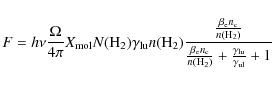
(Liseau & Olofsson 1999). F is the integrated line flux,
|
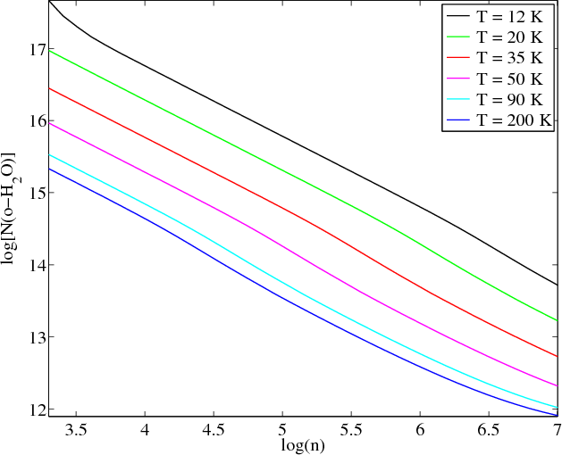
Figure 1:
The derived o-H2O column
density as a function of volume density for different temperatures. The
line intensity for this test case has been set to 0.1 K while
the line width has been set to 10
|
| Open with DEXTER | |
In this study, the temperature is taken from the literature while the
volume density is inferred from CO observations carried out
by others. These two parameters however are not expected to have
constant values across the large Odin beam due to the quite complex
morphology of molecular outflows. For all the sources, we only include
the cosmic microwave background as a radiation field. For simplicity
we have chosen the line intensity to be equal to the peak value while
the line width is taken as the width of the line at 50% of
this
value. The output column density of ortho-water is
then used to
derive the abundance relative to molecular hydrogen, X(o-
![]() )
= N(o-
)
= N(o-
![]() )/N(
)/N(![]() ).
).
A widely used method to obtain the column density for H2
is to
measure the CO abundance assuming a constant universal ratio, e.g.
[
![]() ] = 10-4
(see e.g. Dickman 1978).
In
this paper we use this method where feasible (different methods are
used for TW Hya and 3C391 BML). Volume densities and beam averaged
column densities are estimated from literature data assuming
cylindrical geometry and a mean molecular weight
] = 10-4
(see e.g. Dickman 1978).
In
this paper we use this method where feasible (different methods are
used for TW Hya and 3C391 BML). Volume densities and beam averaged
column densities are estimated from literature data assuming
cylindrical geometry and a mean molecular weight ![]() .
No
correction for inclination is made. The inferred volume densities
(Method 1) should be considered as lower limits for two
reasons. First, the size of the water emitting regions is poorly
known. These regions may very well be smaller than the CO emitting
regions, potentially resulting in a higher average density. Secondly,
shocks, if present, will compress the gas even further. For some of
the sources, there are estimates of the volume density, given in the
literature, that are significantly higher than the ones used in this
paper. In these cases we also estimate an alternative ortho-water
abundance (Method 2).
.
No
correction for inclination is made. The inferred volume densities
(Method 1) should be considered as lower limits for two
reasons. First, the size of the water emitting regions is poorly
known. These regions may very well be smaller than the CO emitting
regions, potentially resulting in a higher average density. Secondly,
shocks, if present, will compress the gas even further. For some of
the sources, there are estimates of the volume density, given in the
literature, that are significantly higher than the ones used in this
paper. In these cases we also estimate an alternative ortho-water
abundance (Method 2).
Table 2
includes the measured integrated intensity over the observed
lines and the derived water abundance. The integrated intensity is
measured over the entire line including the central region as well as
the outflow wings. Exceptions are those outflow sources for which
strong self absorption can be seen (e.g. L1157, Ser SMM1). For these
objects, the integrated intensity has been measured for the red and
the blue wings separately. For sources with no detection, we set
a ![]() upper limit on the integrated intensity in a velocity interval
of 10
upper limit on the integrated intensity in a velocity interval
of 10
![]() (except for TW Hya, where a linewidth of 1
(except for TW Hya, where a linewidth of 1
![]() has
been used).
has
been used).
4.2 Notes on individual sources
4.2.1 L1448
L1448 is a dark cloud in the constellation of Perseus at the distance
of 250 pc (Enoch
et al. 2006). The large, highly collimated outflow
originating from L1448-mm shows enhanced emission from SiO in both
lobes (Nisini et al. 2007).
Franklin et al. (2008)
report o-H2O abundances of X(o-H2O) =
1.5 ![]() 10-6
in the blue wing and
X(o-H2O) =
3.7
10-6
in the blue wing and
X(o-H2O) =
3.7 ![]() 10-6
in the red wing. We report observations
in three positions across the structure, where the northern position
also covers the outflow from L1448 IRS3. The possible detections in
both lobes can, due to instabilities in the baselines, only be
classified as likely. There is also a tentative detection of a bullet
feature in the northern position at
10-6
in the red wing. We report observations
in three positions across the structure, where the northern position
also covers the outflow from L1448 IRS3. The possible detections in
both lobes can, due to instabilities in the baselines, only be
classified as likely. There is also a tentative detection of a bullet
feature in the northern position at ![]()
![]() and
we note that this observation is consistent with the
high speed CO bullet B3 reported by Bachiller
et al. (1990). However,
the preliminary analysis of HCO+ data, recently
taken at the
Onsala Space Observatory, does not reveal any emission at this
velocity. Mass loss rates of M
and
we note that this observation is consistent with the
high speed CO bullet B3 reported by Bachiller
et al. (1990). However,
the preliminary analysis of HCO+ data, recently
taken at the
Onsala Space Observatory, does not reveal any emission at this
velocity. Mass loss rates of M
![]() = 4.6
= 4.6 ![]() 10-6
10-6 ![]() yr-1
for L1448-mm and M
yr-1
for L1448-mm and M
![]() = 1.1
= 1.1 ![]() 10-6
10-6 ![]() yr-1
for L1448 IRS3 were reported by Ceccarelli
et al. (1997)
based on CO observations carried out by Bachiller
et al. (1990).
N(H2) = 6
yr-1
for L1448 IRS3 were reported by Ceccarelli
et al. (1997)
based on CO observations carried out by Bachiller
et al. (1990).
N(H2) = 6 ![]() 1019 cm-2
and n(H2) =
1
1019 cm-2
and n(H2) =
1 ![]() 103 cm-3
are inferred from mass and size estimates
reported by the same authors. We assume the width of the flow to be 40
103 cm-3
are inferred from mass and size estimates
reported by the same authors. We assume the width of the flow to be 40
![]() .
Taking the gas temperature to be T = 37 K
for all
positions (Bachiller
et al. 1995, dust temperature towards
L1448-mm) we derive ortho-water abundances of
between 6
.
Taking the gas temperature to be T = 37 K
for all
positions (Bachiller
et al. 1995, dust temperature towards
L1448-mm) we derive ortho-water abundances of
between 6 ![]() 10-4
and 2
10-4
and 2 ![]() 10-3
in the outflow. Using the higher
volume density (
10-3
in the outflow. Using the higher
volume density (![]() 104)
estimated by Bachiller
et al. (1990),
we derive ortho-water abundances between 1
104)
estimated by Bachiller
et al. (1990),
we derive ortho-water abundances between 1 ![]() 10-4
and 3
10-4
and 3 ![]() 10-4.
10-4.
4.2.2 HH211
The Herbig-Haro jet HH211 is also located in Perseus, 315 pc away (Herbig 1998). It was observed in three different positions enclosing the relatively small outflow. The central and northern beams contain the HH211-mm region. We use the mass estimates from Gueth & Guilloteau (1999) as the basis for our inferred volume densities, n(H2) = 14.2.3 L1551
L1551 is probably one of the most rigorously studied molecular outflows. The main source L1551 IRS5 is located at a distance of 140 pc in the Taurus-Auriga cloud complex (Kenyon et al. 1994). The mass loss rate is in the range 8![\begin{figure}
\par\includegraphics[width=7.5cm,clip]{12064f2.eps} %
\end{figure}](/articles/aa/full_html/2009/45/aa12064-09/img45.png)
|
Figure 2:
The three positions observed by Odin are shown overlaid on a
CO (2-1) map of L1448 (Bachiller
et al. 1995). The circles correspond to the Odin
beam at 557 GHz. Coordinate offsets are given with respect to
L1448-mm: |
| Open with DEXTER | |
4.2.4 TW Hya
At the distance of 56 pc (Qi et al. 2008), TW Hya is the nearest known T Tauri star. Its accretion disk of size 7Not entirely unexpected, Odin did not detect the H2O
557 GHz
line![]() . For representative disk
parameters and a line
width of <1
. For representative disk
parameters and a line
width of <1
![]() ,
the rms of 14 mK would imply an abundance,
X(o-H2O) < 1
,
the rms of 14 mK would imply an abundance,
X(o-H2O) < 1 ![]() 10-8.
For the modeling we used a temperature of 40 K. However,
increasing this parameter to 150 K will not decrease the
derived
upper limit by more than 20%.
10-8.
For the modeling we used a temperature of 40 K. However,
increasing this parameter to 150 K will not decrease the
derived
upper limit by more than 20%.
![\begin{figure}
\par\includegraphics[width=8.8cm,clip]{12064f3.ps}
\end{figure}](/articles/aa/full_html/2009/45/aa12064-09/img52.png)
|
Figure 3:
L1448 spectra. The positions are listed in Table 2 and shown in
Fig. 2.
The letter in the upper right corner indicates in which part of the
flow the spectra were collected (R = red,
B = blue and C = center). The
spectra were baseline subtracted and smoothed to a resolution
of 0.5
|
| Open with DEXTER | |
4.2.5  Cha
I N
Cha
I N
The star forming cloud Chamaeleon I
is located at a distance of
150 pc (Knude &
Hog 1998). From the estimated age (3.8 ![]() 104 yr),
mass (0.21
104 yr),
mass (0.21 ![]() )
and maximum velocity (
)
and maximum velocity (![]() 6
6
![]() )
reported
by Mattila et al.
(1989), we obtain a mass loss rate, M
)
reported
by Mattila et al.
(1989), we obtain a mass loss rate, M
![]() = 3.3
= 3.3 ![]() 10-7
10-7 ![]() yr-1.
The velocity of the wind is
assumed to be 100
yr-1.
The velocity of the wind is
assumed to be 100 ![]() .
We estimate N(H2) = 4
.
We estimate N(H2) = 4 ![]() 1020 cm-2
and n(H2) = 2
1020 cm-2
and n(H2) = 2 ![]() 103 cm-3
from CO observations carried out by
the same authors. The width of the flow is approximately
0.1 pc. Adopting the temperature 50 K, given by Henning et al. (1993),
we obtain an upper limit,
X(o-H2O) < 3
103 cm-3
from CO observations carried out by
the same authors. The width of the flow is approximately
0.1 pc. Adopting the temperature 50 K, given by Henning et al. (1993),
we obtain an upper limit,
X(o-H2O) < 3 ![]() 10-5.
10-5.
![\begin{figure}
\par\includegraphics[width=6.5cm,clip]{12064f4.eps}
\end{figure}](/articles/aa/full_html/2009/45/aa12064-09/img53.png)
|
Figure 4:
The three positions observed by Odin are shown overlaid on a
CO (3-2) map of Sa136 (Parise
et al. 2006). The circles correspond to the Odin
beam at 557 GHz. Coordinate offsets are given with respect to:
|
| Open with DEXTER | |
4.2.6 Sa136 (BHR71)
The Sa136 Bok globule outflows (Sandqvist 1977), at about 200 pc distance, are driven by a binary protostellar system. The secondary CO outflow driven by IRS 2 is more compact (Bourke 2001) than the larger outflow driven by IRS 1.
Taking the column density measurements made by Parise et al. (2006),
assuming a [CO/H2] ratio of ![]() we obtain N(H2) = 1
we obtain N(H2) = 1 ![]() 1021 cm-2,
N(H2) = 4
1021 cm-2,
N(H2) = 4 ![]() 1020 cm-2
and
N(H2) = 3
1020 cm-2
and
N(H2) = 3 ![]() 1021 cm-2
in the red, central and blue
part of the flows respectively. We assume that the flow has a depth of
0.07 pc, yielding volume densities
1021 cm-2
in the red, central and blue
part of the flows respectively. We assume that the flow has a depth of
0.07 pc, yielding volume densities ![]()
![]() 103 cm-3,
103 cm-3,
![]() = 2
= 2 ![]() 103 cm-3
and
103 cm-3
and ![]() = 1
= 1 ![]() 104 cm-3
in the same regions. Parise
et al. (2008) estimate T = 30 -
50 K from CO and methanol observations. In our modeling we use
T =
40 K. We estimate the ortho-water
abundances as (0.1-1)
104 cm-3
in the same regions. Parise
et al. (2008) estimate T = 30 -
50 K from CO and methanol observations. In our modeling we use
T =
40 K. We estimate the ortho-water
abundances as (0.1-1) ![]() 10-5
in the
outflow and 2
10-5
in the
outflow and 2 ![]() 10-4
at the central
position. However, Parise
et al. (2008) give a density of
10-4
at the central
position. However, Parise
et al. (2008) give a density of ![]() = 1
= 1 ![]() 105 cm-3
in the region. Using this higher value we obtain ortho-water
abundances of (2-6)
105 cm-3
in the region. Using this higher value we obtain ortho-water
abundances of (2-6) ![]() 10-7
in the outflow and 3
10-7
in the outflow and 3 ![]() 10-6
towards the central source. The
emission has broader wings in the central position, a feature present
also in the SWAS data. The origin of this high velocity component
and the elevated water abundance might be the smaller outflow
originating from IRS 2, visible in Fig. 4. Based on
the outflow mass (1.3
10-6
towards the central source. The
emission has broader wings in the central position, a feature present
also in the SWAS data. The origin of this high velocity component
and the elevated water abundance might be the smaller outflow
originating from IRS 2, visible in Fig. 4. Based on
the outflow mass (1.3 ![]() ), dynamical time scale
(1
), dynamical time scale
(1 ![]() 104 yr)
and
flow velocity (28
104 yr)
and
flow velocity (28
![]() )
provided by
Bourke et al. (1997)
)
provided by
Bourke et al. (1997)![]() for the larger flows, we
estimate the mass loss
rate to be M
for the larger flows, we
estimate the mass loss
rate to be M
![]() = 3.6
= 3.6 ![]() 10-5
10-5 ![]() yr-1.
The
wind velocity is assumed to be 100
yr-1.
The
wind velocity is assumed to be 100
![]() .
.
![\begin{figure}
\par\includegraphics[width=8cm,clip]{12064f5.ps}
\end{figure}](/articles/aa/full_html/2009/45/aa12064-09/img58.png)
|
Figure 5: The same as Fig. 3 but for Sa136. |
| Open with DEXTER | |
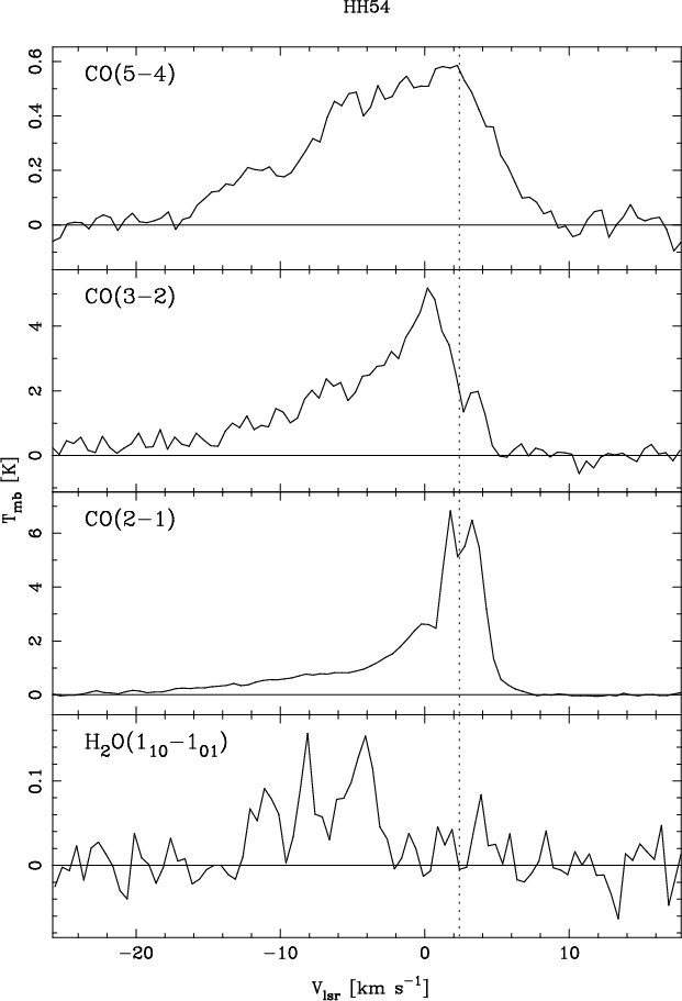
4.2.7 HH54 B
The Herbig-Haro object HH54 B is situated in the Cha
II cloud
at roughly 200 pc (Hughes
& Hartigan 1992). During the observations, the
correlator suffered from ripple. This had the effect of increasing the
line intensity and a substantial amount of data had to be
abandoned. The signal detected can therefore only be classified as
tentative although we are confident that the data do not show any
systematic variations. Complementary data were obtained in CO(3-2),
CO(2-1), SiO(5-4), SiO(3-2) and SiO(2-1) with the SEST telescope
(see Appendix A)
and in CO(5-4) with Odin. The
CO(5-4) data suffer from frequency drift, something that adds an
![]() 10
10
![]() uncertainty to our velocity scale. However, we do
not believe that this gives large uncertainties on the line strength.
uncertainty to our velocity scale. However, we do
not believe that this gives large uncertainties on the line strength.
No shock-enhanced emission was detected in any of the observed SiO transitions. This result seems not easily reconcilable with the prediction from theoretical C-shock models (see Fig. 6 of Gusdorf et al. 2008), which appear closely adaptable to the conditions in HH 54 (Neufeld et al. 2006; Liseau et al. 1996).
Both the CO (2-1) and (3-2) lines show an absorption
feature at
+2.4
![]() ,
which corresponds to the LSR-velocity
of the molecular cloud. In addition, a strong blue wing is observed in
all positions, but essentially no redshifted gas, which is in
agreement with the (1-0) observations by Knee
(1992). Both
(2-1) and (3-2) transitions peak at the central map position, i.e. on
HH 54B itself and their integrated intensities,
,
which corresponds to the LSR-velocity
of the molecular cloud. In addition, a strong blue wing is observed in
all positions, but essentially no redshifted gas, which is in
agreement with the (1-0) observations by Knee
(1992). Both
(2-1) and (3-2) transitions peak at the central map position, i.e. on
HH 54B itself and their integrated intensities, ![]() ,
are given in Table A.1.
,
are given in Table A.1.
|
Figure 6:
From top to bottom the CO(5-4), CO(3-2),
CO(2-1) and |
| Open with DEXTER | |
For the comparison with the ISO-LWS model of Liseau et al. (1996),
we
use the average radiation temperature, approximated by ![]() .
This yields
.
This yields ![]() K
and
K
and ![]() K
for the
CO (2-1) and (3-2) lines, respectively. Both values
are smaller, by 25% and 40% respectively, than the model
predictions of 1.6 K and
5.7 K, which were based on a single-temperature approximation.
Even
though the strength of the CO(5-4) line is uncertain, it shows
a
slightly higher temperature than the predicted 0.3 K. Putting
it all
together, the model predicts the radiation temperature in all three
lines to within an order of 2. For the RADEX
analysis we use the
ISO-LWS model T = 330 K, n(H2) = 2
K
for the
CO (2-1) and (3-2) lines, respectively. Both values
are smaller, by 25% and 40% respectively, than the model
predictions of 1.6 K and
5.7 K, which were based on a single-temperature approximation.
Even
though the strength of the CO(5-4) line is uncertain, it shows
a
slightly higher temperature than the predicted 0.3 K. Putting
it all
together, the model predicts the radiation temperature in all three
lines to within an order of 2. For the RADEX
analysis we use the
ISO-LWS model T = 330 K, n(H2) = 2 ![]() 105 cm-3
and
N(H2) = 3
105 cm-3
and
N(H2) = 3 ![]() 1019 cm-2,
where the column density has been
diluted to the Odin beam. We obtain a beam averaged water abundance
of X(o-H2O) = 3
1019 cm-2,
where the column density has been
diluted to the Odin beam. We obtain a beam averaged water abundance
of X(o-H2O) = 3 ![]() 10-6.
However, recently
Neufeld et al. (2006)
estimate a higher H2 column density for the
warm gas, a fact that could alter our derived abundance by an order of
magnitude downwards. The mass loss rate of the unknown driving source
has been estimated by Giannini
et al. (2006) as M
10-6.
However, recently
Neufeld et al. (2006)
estimate a higher H2 column density for the
warm gas, a fact that could alter our derived abundance by an order of
magnitude downwards. The mass loss rate of the unknown driving source
has been estimated by Giannini
et al. (2006) as M
![]()
![]() yr-1.
yr-1.
4.2.8 G327.3-0.6
The hot core G327.3-0.6 is located in the southern hemisphere at the distance of 2.9 kpc (Bergman 1992). CO line profiles obtained by Wyrowski et al. (2006) weakly indicate the presence of outflows, however, to date there has been no further study of this. From CO observations performed by these authors, we infer N(H2) = 24.2.9 NGC 6334 I
At least two outflows are emerging from NGC 6334 I,
located in
the constellation Scorpius (McCutcheon
et al. 2000) at the distance
of 1.7 kpc (Neckel 1978).
From CO observations provided by
Leurini et al. (2006)
we obtain a beam averaged column density
1 ![]() 1020 cm-2
and a volume density 4
1020 cm-2
and a volume density 4 ![]() 103 cm-3.
We
assume that the gas temperature is the same as the dust temperature,
viz. T = 100 K (Sandell 2000). This is
consistent with
Leurini et al. (2006)
who set a lower limit on the kinetic
temperature at 50 K. With the above properties we derive an
abundance
of X(o-H2O) = 5
103 cm-3.
We
assume that the gas temperature is the same as the dust temperature,
viz. T = 100 K (Sandell 2000). This is
consistent with
Leurini et al. (2006)
who set a lower limit on the kinetic
temperature at 50 K. With the above properties we derive an
abundance
of X(o-H2O) = 5 ![]() 10-5.
10-5.
The baseline subtracted spectrum does not show any evidence of
high
velocity gas. However, we do not find this easily reconcilable with
the high velocity gas detected in several CO transitions by
Leurini et al. (2006).
One possibility could be the curved baseline
hiding the outflow wings. Therefore, we investigate also an
alternative case where we assume that the entire curvature stems from
the outflowing gas. This secondary scenario is perhaps not very
likely. However, at present it is not possible to draw any firm
conclusions. The estimated depth of the absorption feature is greater
than the continuum level of 360 Jy, interpolated from
800 ![]() m
observations provided by Sandell
(2000). In this secondary
case we derive the abundance X(o-H2O) = 2
m
observations provided by Sandell
(2000). In this secondary
case we derive the abundance X(o-H2O) = 2 ![]() 10-3.
10-3.
| Figure 7: The same as Fig. 3 but for NGC 6334 I. The black spectrum represents the first case and the grey spectrum represents the second case as described in Sect. 4.2.9 |
|
| Open with DEXTER | |
4.2.10 Ser SMM1
The Serpens star forming dark cloud is situated in the inner Galaxy at
a distance of 310 pc (de
Lara et al. 1991). Franklin
et al. (2008)
estimated ortho-water abundances of X(o-H2O) = 7.1 ![]() 10-7
and
X(o-H2O) = 3.8
10-7
and
X(o-H2O) = 3.8 ![]() 10-7
in the blue and red wing respectively
while Larsson et al.
(2002) estimate the water abundance as
X(H2O) = 1
10-7
in the blue and red wing respectively
while Larsson et al.
(2002) estimate the water abundance as
X(H2O) = 1 ![]() 10-5
in the region. Davis
et al. (1999) provide
the mass and size of the outflow based on CO observations.
Assuming a
width of 0.2 pc yields n(H2) = 1
10-5
in the region. Davis
et al. (1999) provide
the mass and size of the outflow based on CO observations.
Assuming a
width of 0.2 pc yields n(H2) = 1 ![]() 103 cm-3
and
N(H2) = 5
103 cm-3
and
N(H2) = 5 ![]() 1020 cm-2.
From O I(63
1020 cm-2.
From O I(63 ![]() m)
measurements carried out by Larsson
et al. (2002, and references
therein) we obtain the mass loss rate, M
m)
measurements carried out by Larsson
et al. (2002, and references
therein) we obtain the mass loss rate, M
![]() = 3
= 3 ![]() 10-7
10-7 ![]() yr-1.
The temperature of the dust
was constrained by White
et al. (1995) to be
30 K < T < 40 K.
Using T = 35 K and the above properties we
obtain
X(o-H2O) = 9
yr-1.
The temperature of the dust
was constrained by White
et al. (1995) to be
30 K < T < 40 K.
Using T = 35 K and the above properties we
obtain
X(o-H2O) = 9 ![]() 10-5
and X(o-H2O) = 5
10-5
and X(o-H2O) = 5 ![]() 10-5
in the blue
and red flow.
10-5
in the blue
and red flow.
| Figure 8: The same as Fig. 3 but for Ser SMM1. |
|
| Open with DEXTER | |
![\begin{figure}
\par\includegraphics[width=7cm,clip]{12064f9.eps}
\end{figure}](/articles/aa/full_html/2009/45/aa12064-09/img69.png)
|
Figure 9:
The four positions observed by Odin are shown overlaid on a
CO (2-1) map of L1157 (Bachiller
et al. 2001). The circles correspond to the Odin
beam at 557 GHz. Coordinate offsets are given with respect to
L1157-mm, indicated in the figure with a star symbol: |
| Open with DEXTER | |
4.2.11 B335
The dense core in the B335 globule is believed to be one of the major candidates for protostellar collapse. This isolated source at the distance of 150 pc (Stutz et al. 2008) harbors several Herbig-Haro objects associated with a bipolar outflow (see e.g. Gålfalk & Olofsson 2007). Following the outflow mass estimate of 0.444.2.12 L1157
![\begin{figure}
\par\includegraphics[width=7.4cm,clip]{12064f10.ps}
\end{figure}](/articles/aa/full_html/2009/45/aa12064-09/img72.png)
|
Figure 10: The same as Fig. 3 but for L1157. |
| Open with DEXTER | |
L1157 is a Class 0 object in the constellation of Cepheus situated at
a distance of 250 pc (Looney
et al. 2007). It drives a prototype
bipolar outflow which was observed by Odin in four different
positions. The mass loss rate can be derived from mass (0.62 ![]() )
and time scale (15 000 yr) estimations given by
Bachiller et al.
(2001). Assuming a maximum CO velocity of 20
)
and time scale (15 000 yr) estimations given by
Bachiller et al.
(2001). Assuming a maximum CO velocity of 20
![]() and a stellar wind velocity of 100 km s-1,
we derive
M
and a stellar wind velocity of 100 km s-1,
we derive
M
![]() = 8.3
= 8.3 ![]() 10-6
10-6 ![]() yr-1
. The Odin strip
map covers the bulk of the outflow with two pointings in the red wing,
one in the blue, and one on the driving source of the outflow itself
(Fig. 9).
The observations were carried out using the
AOS and the AC2 simultaneously. The spectra shown in
Fig. 10
are the averages of the merged data.
The total mass in the different parts of the flow were obtained from
CO observations carried out by Bachiller
et al. (2001). From this we
estimate n(H2) = 2
yr-1
. The Odin strip
map covers the bulk of the outflow with two pointings in the red wing,
one in the blue, and one on the driving source of the outflow itself
(Fig. 9).
The observations were carried out using the
AOS and the AC2 simultaneously. The spectra shown in
Fig. 10
are the averages of the merged data.
The total mass in the different parts of the flow were obtained from
CO observations carried out by Bachiller
et al. (2001). From this we
estimate n(H2) = 2 ![]() 103 cm-3
and N(H2) = 2
103 cm-3
and N(H2) = 2 ![]() 1020 cm-2
in the northern lobe, while n(H2) = 3
1020 cm-2
in the northern lobe, while n(H2) = 3 ![]() 103 cm-3
and N(H2) = 2
103 cm-3
and N(H2) = 2 ![]() 1020 cm-2
in the
central and southern region. The size of the CO outflow is
taken to be
50
1020 cm-2
in the
central and southern region. The size of the CO outflow is
taken to be
50
![]()
![]() 375
375
![]() .
For all four positions we set the kinetic
temperature to T = 30 K, a rough global
estimate based on
Bachiller et al.
(2001). We calculate the abundances in the outflow
to be within the range of
.
For all four positions we set the kinetic
temperature to T = 30 K, a rough global
estimate based on
Bachiller et al.
(2001). We calculate the abundances in the outflow
to be within the range of ![]() and
and ![]() .
The derived water abundance in the central region is
slightly lower, X(o-H2O) = 2
.
The derived water abundance in the central region is
slightly lower, X(o-H2O) = 2 ![]() 10-4
in the blue lobe and
X(o-H2O) = 3
10-4
in the blue lobe and
X(o-H2O) = 3 ![]() 10-5
in the red. The increased blue emission
likely originates from the outflow. Within the Odin beam are the
positions B0 and B1 that show peaked emission in H2CO,
CS,
CH3OH, SO (Bachiller
et al. 2001, their Fig. 1) and SiO
(Nisini et al. 2007).
Franklin et al. (2008)
estimated X(o-H2O) = 8.0
10-5
in the red. The increased blue emission
likely originates from the outflow. Within the Odin beam are the
positions B0 and B1 that show peaked emission in H2CO,
CS,
CH3OH, SO (Bachiller
et al. 2001, their Fig. 1) and SiO
(Nisini et al. 2007).
Franklin et al. (2008)
estimated X(o-H2O) = 8.0 ![]() 10-6
and X(o-H2O) = 9.7
10-6
and X(o-H2O) = 9.7 ![]() 10-6
in the blue and red
wing respectively.
10-6
in the blue and red
wing respectively.
Bachiller
et al. (2001) estimates the density around the
protostar
to be ![]() 106 cm-3.
When moving from B0 to B2, the
density changes from
106 cm-3.
When moving from B0 to B2, the
density changes from ![]() 3
to 6
3
to 6 ![]() 105 cm-3.
Using
n(H2) = 1
105 cm-3.
Using
n(H2) = 1 ![]() 106 cm-3
and n(H2) =
5
106 cm-3
and n(H2) =
5 ![]() 105 cm-3
for the central and southern part respectively
we obtain the abundances X(o-H2O) = 5
105 cm-3
for the central and southern part respectively
we obtain the abundances X(o-H2O) = 5 ![]() 10-7
and X(o-H2O) = 2
10-7
and X(o-H2O) = 2 ![]() 10-6.
10-6.
4.2.13 NGC 7538 IRS1
NGC 7538 IRS1 is a region of ongoing high mass star formation. The main infrared source IRS1 is located at the boundary of an H II region in the Perseus arm, located at a distance of 2.7 kpc (Moscadelli et al. 2008). In addition to IRS1, and its high velocity outflow, also several other sub-mm sources fall into the large Odin beam. The mass loss rate from IRS1 was estimated by Kameya et al. (1989) to be M| Figure 11: The same as Fig. 3 but for NGC 7538 IRS1. |
|
| Open with DEXTER | |
4.2.14 Supernova remnants
3C391 BML is a supernova remnant at a distance of 8 kpc (Chen & Slane 2001). The temperature, volume density and column density of the gas were constrained to 50 KIC443 is a shell type supernova remnant at the
distance of about 1.5 kpc (Fesen
1984). The broad emission
peaks are labeled A through H, where Odin has observed clump G. The
volume density and temperature were modeled by
van Dishoeck
et al. (1993) as n(H2) = 5 ![]() 105 cm-3
and
T = 100 K. Using the CO column density
inferred by the same
authors, assuming a
105 cm-3
and
T = 100 K. Using the CO column density
inferred by the same
authors, assuming a ![]() ratio of
ratio of ![]() and a
source size of 40
and a
source size of 40
![]()
![]() 100
100
![]() ,
we obtain N(H2) = 3
,
we obtain N(H2) = 3 ![]() 1021
cm-2. The derived abundance is X(o-
1021
cm-2. The derived abundance is X(o-
![]() .
This is in agreement with
Snell et al. (2005)
who derive an o-H2O
abundance with respect to
12CO, X(o-H2O) = 3.7
.
This is in agreement with
Snell et al. (2005)
who derive an o-H2O
abundance with respect to
12CO, X(o-H2O) = 3.7 ![]() 10-4.
10-4.
| Figure 12: The same as Fig. 3 but for IC443-G. |
|
| Open with DEXTER | |
4.3 Water abundance
The water abundances inferred from our analysis are given with respect to the molecular column density within the Odin beam. The values span a wide range with most of the sources having an abundance of the orderAssuming an inclination angle of 60![]() with respect to the line
of sight for all the targets, we plot the o-H2O
abundances versus
the maximum velocities (Fig. 13). The
maximum
velocities are taken from the spectra as the maximum offsets between
the cloud velocity and the flow velocity. There is a correlation
between the derived abundances and the maximum velocities of the
outflowing gas. The solid line in Fig. 13 is the
first order polynomial least square fit:
with respect to the line
of sight for all the targets, we plot the o-H2O
abundances versus
the maximum velocities (Fig. 13). The
maximum
velocities are taken from the spectra as the maximum offsets between
the cloud velocity and the flow velocity. There is a correlation
between the derived abundances and the maximum velocities of the
outflowing gas. The solid line in Fig. 13 is the
first order polynomial least square fit:
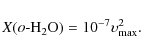
|
(2) |
The correlation coefficient is 0.57 while the p-value, testing the hypothesis of no correlation is 0.04. Following the C-shock modelling carried out by Kaufman & Neufeld (1996), a relationship is expected when shocks are responsible for the emission. However, the abundances do not show any tendency to level off with velocities greater than

|
Figure 13:
o-H2O abundance plotted
against the maximum velocity for an overall inclination of 60 |
| Open with DEXTER | |
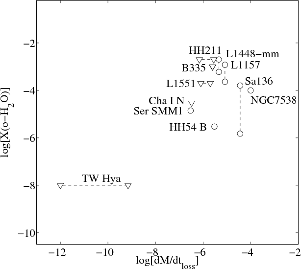
|
Figure 14: o-H2O abundance plotted against the mass loss rate. The triangles represent the high upper limits for each source in the o-H2O abundance, while the circles symbolize values where a detection has been made. Dashed lines represent the cases where there is a range in the inferred abundances or mass loss rates. |
| Open with DEXTER | |
4.4 Comparison with SWAS data
For all the outflows except TW Hya the gas volume density, used as an input parameter to RADEX, has been derived from CO observations. This method generally underestimates the mass of the regions. The possibility that the water emission originates from gas with a higher volume density than this can therefore not be ruled out. Nevertheless, we are confident that the volume density does span a wide range of values. This is also one of the reasons why several of our derived abundances deviate from those inferred by Franklin et al. (2008). They use a single volume density of n(H2) = 105 cm-3 and our values differ from this by more than two orders of magnitude for some of the sources (see Table 2). Figure 15 shows a histogram of the numbers of sources within different volume density ranges. The difficulty to estimate the gas column density of the water emitting regions is a problem that has to be adressed in order to interpret future observations with Herschel.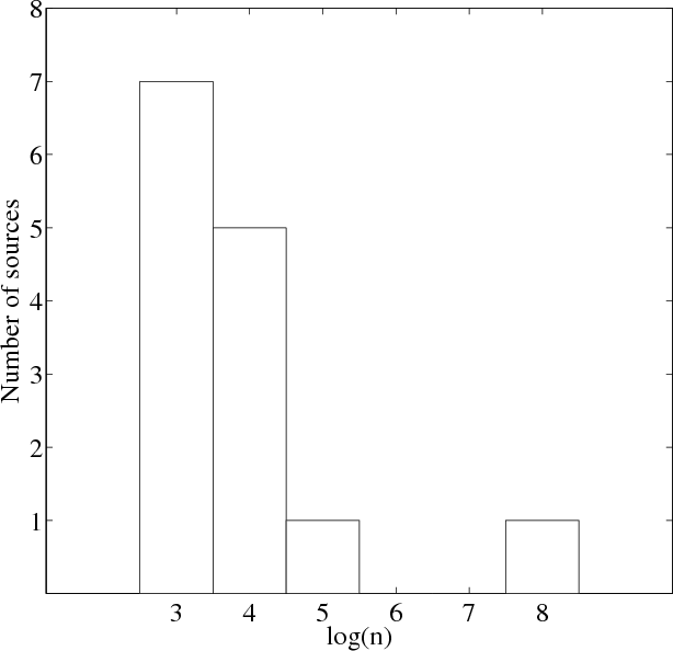
|
Figure 15: A histogram of the gas volume density estimated in the outflows studied in this paper showing a variation that spans over six orders of magnitude. |
| Open with DEXTER | |
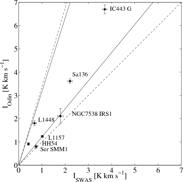
The integrated intensities for the SWAS and Odin outflow spectra
are compared in Fig. 16 to
provide an estimate of
the source size of the water emitting regions. The dashed
1:1 ratio
line illustrates the case where the source fills both antenna
beams while the dashed 3.37:1 line indicates a small source
size
compared to both beams. Assuming that both the emitting sources and
the antenna responses are circularly symmetric and Gaussian, these
ratios follow from the relation:
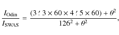
where
|
Figure 16: Integrated intensities for common sources of Odin and SWAS. The dashed lines show the 3.37:1 and the 1:1 ratios between the Odin and SWAS integrated intensities. The error bars refer to the analysis and the solid lines represents ratios 1:1 and 3.37:1 with a 15% uncertainty applied. This is the estimated error limit from the data reduction. |
| Open with DEXTER | |
4.5 Outflows and observed water abundances
The main objective for these observations is to use the ground state o-H2O transition as a tracer for shocked gas. Available shock models by Bergin et al. (1998) show that a shock velocity in excess of 105 Conclusions
We make the following primary conclusions:- 1.
- We have observed 13 outflows and two supernova remnants and detect the ortho-water ground state rotational transition in seven outflows and one supernova remnant.
- 2.
- The column densities of o-H2O have been investigated with RADEX , having the volume density, temperature, line intensity and linewidth as input. Elevated abundances of water are found in several sources. The abundances are as high as one would expect if all gaseous oxygen had been converted to water in a C-type shock.
- 3.
- There is no distinct relationship between the water abundance and the mass loss rate.
- 4.
- There is a correlation between the o-H2O abundance and the maximum velocity of the gas.
The author enjoyed interesting discussions with John H. Black concerning radiative transfer in general and RADEX in particular. Carina M. Persson and Per Bergman are also acknowledged. We thank the Research Councils and Space Agencies in Sweden, Canada, Finland and France for their financial support. The valuable comments made by the anonymous referee are highly appreciated.
Appendix A: Ground based observations
The observations with the Swedish ESO Submillimetre Telescope (SEST) were made during 11-20 August 1997 and 2-6 August 1998. Some complementary SiO (2-1) map data were collected during 7-9 February 2003. The observed molecules and their transitions are listed in Table A.1 and for SiO (2-1) and (3-2), the observations were made simultaneously.
Table A.1: Molecular line observations with the 15 m SEST.
SIS receivers were used as frontends and the backend was aThe data were chopper-wheel calibrated in the ![]() -scale (Ulich & Haas 1976)
and the main beam
efficiencies at the different frequencies,
-scale (Ulich & Haas 1976)
and the main beam
efficiencies at the different frequencies, ![]() ,
are given
in Table A.1.
The pointing of the telescope was regularly
checked towards point sources, masing in the SiO (v=1,
J=2-1) line,
and was determined to be better than 3
,
are given
in Table A.1.
The pointing of the telescope was regularly
checked towards point sources, masing in the SiO (v=1,
J=2-1) line,
and was determined to be better than 3
![]() (rms). However, for
HH 54, all SiO data refer to the vibrational ground state, v=0,
and
the (2-1) and (3-2) data were obtained in frequency switching mode,
with a frequency chop of 4 MHz.
(rms). However, for
HH 54, all SiO data refer to the vibrational ground state, v=0,
and
the (2-1) and (3-2) data were obtained in frequency switching mode,
with a frequency chop of 4 MHz.
Knee (1992)
assigned a kinetic gas temperature of ![]() 15 K
to the bulk cloud material. In the CO (3-2) line,
this should yield a
high contrast between the cloud and the high velocity gas. To achieve
flat, optimum baselines, the CO (3-2) observations therefore
were made
in wide dual beam switching with throws of
15 K
to the bulk cloud material. In the CO (3-2) line,
this should yield a
high contrast between the cloud and the high velocity gas. To achieve
flat, optimum baselines, the CO (3-2) observations therefore
were made
in wide dual beam switching with throws of ![]() 11
11![]() in
azimuth. At this maximum amplitude available at the SEST, the
reference beams were still inside the molecular cloud. For this
reason, this mode could not be adopted for the CO (2-1)
observations,
which were performed in total power mode. The reference position
was 1
in
azimuth. At this maximum amplitude available at the SEST, the
reference beams were still inside the molecular cloud. For this
reason, this mode could not be adopted for the CO (2-1)
observations,
which were performed in total power mode. The reference position
was 1![]() north of HH 54. Centered on the object, nine point maps with
25
north of HH 54. Centered on the object, nine point maps with
25
![]() spacings were obtained in both CO lines. In addition, a
tighter sampled nine point map with 15
spacings were obtained in both CO lines. In addition, a
tighter sampled nine point map with 15
![]() spacings was also made in
CO (3-2).
spacings was also made in
CO (3-2).
HH54 B was observed again on June 8th to June 11th, 2009.
8.2 h of integration time confirmed the presence of the H![]() O
557 GHz line. Adding all observations results in an
integrated intensity of
O
557 GHz line. Adding all observations results in an
integrated intensity of ![]() K
K
![]() .
.
References
- Bachiller, R., Guilloteau, S., & Kahane, C. 1987, A&A, 173, 324 [NASA ADS]
- Bachiller, R., Martin-Pintado, J., Tafalla, M., Cernicharo, J., & Lazareff, B. 1990, A&A, 231, 174 [NASA ADS]
- Bachiller, R., Guilloteau, S., Dutrey, A., Planesas, P., & Martin-Pintado, J. 1995, A&A, 299, 857 [NASA ADS]
- Bachiller, R., Pérez Gutiérrez, M., Kumar, M. S. N., & Tafalla, M. 2001, A&A, 372, 899 [NASA ADS] [CrossRef] [EDP Sciences]
- Benedettini, M., Viti, S., Giannini, T., et al. 2002, A&A, 395, 657 [NASA ADS] [CrossRef] [EDP Sciences]
- Bergin, E. A., Neufeld, D. A., & Melnick, G. J. 1998, ApJ, 499, 777 [NASA ADS] [CrossRef]
- Bergman, P. 1992, Ph.D. Thesis, Göteborg, Sweden
- Bourke, T. L., Garay, G., Lehtinen, K. K., et al. 1997, ApJ, 476, 781 [NASA ADS] [CrossRef]
- Bourke, T. L. 2001, ApJ, 554, L91 [NASA ADS] [CrossRef]
- Ceccarelli, C., Haas, M. R., Hollenbach, D. J., & Rudolph, A. L. 1997, ApJ, 476, 771 [NASA ADS] [CrossRef]
- Chen, Y., & Slane, P. O. 2001, ApJ, 563, 202 [NASA ADS] [CrossRef]
- Davis, C. J., Matthews, H. E., Ray, T. P., Dent, W. R. F., & Richer, J. S. 1999, MNRAS, 309, 141 [NASA ADS] [CrossRef]
- de la Reza, R., Jilinski, E., & Ortega, V. G. 2006, AJ, 131, 2609 [NASA ADS] [CrossRef]
- de Lara, E., Chavarria-K., C., & Lopez-Molina, G. 1991, A&A, 243, 139 [NASA ADS]
- Dickman, R. L. 1978, ApJS, 37, 407 [NASA ADS] [CrossRef]
- Dubernet, M.-L., & Grosjean, A. 2002, A&A, 390, 793 [NASA ADS] [CrossRef] [EDP Sciences]
- Dubernet, M.-L., Daniel, F., Grosjean, A., & Lin, C. Y. 2009, A&A, 497, 911 [NASA ADS] [CrossRef] [EDP Sciences]
- Dupree, A. K., Brickhouse, N. S., Smith, G. H., & Strader, J. 2005, ApJ, 625, L131 [NASA ADS] [CrossRef]
- Enoch, M. L., Young, K. E., Glenn, J., et al. 2006, ApJ, 638, 293 [NASA ADS] [CrossRef]
- Evans, II, N. J., Lee, J.-E., Rawlings, J. M. C., & Choi, M. 2005, ApJ, 626, 919 [NASA ADS] [CrossRef]
- Faure, A., Crimier, N., Ceccarelli, C., et al. 2007, A&A, 472, 1029 [NASA ADS] [CrossRef] [EDP Sciences]
- Fesen, R. A. 1984, ApJ, 281, 658 [NASA ADS] [CrossRef]
- Franklin, J., Snell, R. L., Kaufman, M. J., et al. 2008, ApJ, 674, 1015 [NASA ADS] [CrossRef]
- Frisk, U., Hagström, M., Ala-Laurinaho, J., et al. 2003, A&A, 402, L27 [NASA ADS] [CrossRef] [EDP Sciences]
- Gålfalk, M., & Olofsson, G. 2007, A&A, 475, 281 [NASA ADS] [CrossRef] [EDP Sciences]
- Giannini, T., McCoey, C., Nisini, B., et al. 2006, A&A, 459, 821 [NASA ADS] [CrossRef] [EDP Sciences]
- Gueth, F., & Guilloteau, S. 1999, A&A, 343, 571 [NASA ADS]
- Gusdorf, A., Cabrit, S., Flower, D. R., & Pineau Des Forêts, G. 2008, A&A, 482, 809 [NASA ADS] [CrossRef] [EDP Sciences]
- Hartstein, D., & Liseau, R. 1998, A&A, 332, 703 [NASA ADS]
- Henning, T., Pfau, W., Zinnecker, H., & Prusti, T. 1993, A&A, 276, 129 [NASA ADS]
- Herbig, G. H. 1998, ApJ, 497, 736 [NASA ADS] [CrossRef]
- Herczeg, G. J., Wood, B. E., Linsky, J. L., Valenti, J. A., & Johns-Krull, C. M. 2004, ApJ, 607, 369 [NASA ADS] [CrossRef]
- Hirano, N., Kameya, O., Nakayama, M., & Takakubo, K. 1988, ApJ, 327, L69 [NASA ADS] [CrossRef]
- Hjalmarson, Å., Frisk, U., Olberg, M., et al. 2003, A&A, 402, L39 [NASA ADS] [CrossRef] [EDP Sciences]
- Hughes, J., & Hartigan, P. 1992, AJ, 104, 680 [NASA ADS] [CrossRef]
- Kameya, O., Hasegawa, T. I., Hirano, N., Takakubo, K., & Seki, M. 1989, ApJ, 339, 222 [NASA ADS] [CrossRef]
- Kastner, J. H., Zuckerman, B., Weintraub, D. A., & Forveille, T. 1997, Science, 277, 67 [NASA ADS] [CrossRef]
- Kaufman, M. J., & Neufeld, D. A. 1996, ApJ, 456, 611 [NASA ADS] [CrossRef]
- Kenyon, S. J., Dobrzycka, D., & Hartmann, L. 1994, AJ, 108, 1872 [NASA ADS] [CrossRef]
- Kessler, M. F., Steinz, J. A., Anderegg, M. E., et al. 1996, A&A, 315, L27 [NASA ADS]
- Klotz, A., Harju, J., Ristorcelli, I., et al. 2008, A&A, 488, 559 [NASA ADS] [CrossRef] [EDP Sciences]
- Knee, L. B. G. 1992, A&A, 259, 283 [NASA ADS]
- Knude, J., & Hog, E. 1998, A&A, 338, 897 [NASA ADS]
- Lamzin, S. A., Kravtsova, A. S., Romanova, M. M., & Batalha, C. 2004, Astron. Lett., 30, 413 [NASA ADS] [CrossRef]
- Larsson, B., Liseau, R., & Men'shchikov, A. B. 2002, A&A, 386, 1055 [NASA ADS] [CrossRef] [EDP Sciences]
- Leurini, S., Schilke, P., Parise, B., et al. 2006, A&A, 454, L83 [CrossRef] [EDP Sciences]
- Lee, C.-F., Ho, P. T. P., Palau, A., et al. 2007, ApJ, 670, 1188 [NASA ADS] [CrossRef]
- Linke, R. A., Goldsmith, P. F., Wannier, P. G., Wilson, R. W., & Penzias, A. A. 1977, ApJ, 214, 50 [NASA ADS] [CrossRef]
- Liseau, R., & Olofsson, G. 1999, A&A, 343, L83 [NASA ADS]
- Liseau, R., Ceccarelli, C., Larsson, B., et al. 1996, A&A, 315, L181 [NASA ADS]
- Liseau, R., Fridlund, C. V. M., & Larsson, B. 2005, ApJ, 619, 959 [NASA ADS] [CrossRef]
- Lockett, P., Gauthier, E., & Elitzur, M. 1999, ApJ, 511, 235 [NASA ADS] [CrossRef]
- Looney, L. W., Tobin, J. J., & Kwon, W. 2007, ApJ, 670, L131 [NASA ADS] [CrossRef]
- Mattila, K., Liljeström, T., & Toriseva, M. 1989, in Low Mass Star Formation and Pre-main Sequence Objects, ed. B. Reipurth, 153
- McCutcheon, W. H., Sandell, G., Matthews, H. E., et al. 2000, MNRAS, 316, 152 [NASA ADS] [CrossRef]
- Melnick, G. J., Stauffer, J. R., Ashby, M. L. N., et al. 2000, ApJ, 539, L77 [NASA ADS] [CrossRef]
- Moscadelli, L., Reid, M. J., Menten, K. M., et al. 2008, ArXiv e-prints
- Neckel, T. 1978, A&A, 69, 51 [NASA ADS]
- Neufeld, D. A., Melnick, G. J., Sonnentrucker, P., et al. 2006, ApJ, 649, 816 [NASA ADS] [CrossRef]
- Nisini, B., Codella, C., Giannini, T., et al. 2007, A&A, 462, 163 [NASA ADS] [CrossRef] [EDP Sciences]
- Nordh, H. L., von Schéele, F., Frisk, U., et al. 2003, A&A, 402, L21 [NASA ADS] [CrossRef] [EDP Sciences]
- Olberg, M., Frisk, U., Lecacheux, A., et al. 2003, A&A, 402, L35 [NASA ADS] [CrossRef] [EDP Sciences]
- Olofsson, A. O. H., Olofsson, G., Hjalmarson, Å., et al. 2003, A&A, 402, L47 [NASA ADS] [CrossRef] [EDP Sciences]
- Parise, B., Belloche, A., Leurini, S., et al. 2006, A&A, 454, L79 [NASA ADS] [CrossRef] [EDP Sciences]
- Parise, B., Belloche, A., Leurini, S., & Schilke, P. 2008, Ap&SS, 313, 73 [NASA ADS] [CrossRef]
- Persson, C. M., Olberg, M., Hjalmarson, Ã., et al. 2009, A&A, 494, 637 [NASA ADS] [CrossRef] [EDP Sciences]
- Phillips, T. R., Maluendes, S., & Green, S. 1996, ApJS, 107, 467 [NASA ADS] [CrossRef]
- Qi, C., Wilner, D. J., Aikawa, Y., Blake, G. A., & Hogerheijde, M. R. 2008, ApJ, 681, 1396 [NASA ADS] [CrossRef]
- Ristorcelli, I., Falgarone, E., Schöier, F., et al. 2005, in IAU Symp., 235, 227
- Sandell, G. 2000, A&A, 358, 242 [NASA ADS]
- Sandell, G., & Sievers, A. 2004, ApJ, 600, 269 [NASA ADS] [CrossRef]
- Sandqvist, A. 1977, A&A, 57, 467 [NASA ADS]
- Snell, R. L., Loren, R. B., & Plambeck, R. L. 1980, ApJ, 239, L17 [NASA ADS] [CrossRef]
- Snell, R. L., Howe, J. E., Ashby, M. L. N., et al. 2000, ApJ, 539, L93 [NASA ADS] [CrossRef]
- Snell, R. L., Hollenbach, D., Howe, J. E., et al. 2005, ApJ, 620, 758 [NASA ADS] [CrossRef]
- Stojimirovic, I., Narayanan, G., Snell, R. L., & Bally, J. 2006, ApJ, 649, 280 [NASA ADS] [CrossRef]
- Stutz, A. M., Rubin, M., Werner, M. W., et al. 2008, ApJ, 687, 389 [NASA ADS] [CrossRef]
- Ulich, B. L., & Haas, R. W. 1976, ApJS, 30, 247 [NASA ADS] [CrossRef]
- van der Tak, F. F. S., Black, J. H., Schöier, F. L., Jansen, D. J., & van Dishoeck, E. F. 2007, A&A, 468, 627 [NASA ADS] [CrossRef] [EDP Sciences]
- van Dishoeck, E. F., Jansen, D. J., & Phillips, T. G. 1993, A&A, 279, 541 [NASA ADS]
- van Zadelhoff, G.-J., van Dishoeck, E. F., Thi, W.-F., & Blake, G. A. 2001, A&A, 377, 566 [NASA ADS] [CrossRef] [EDP Sciences]
- Werner, M. W., Roellig, T. L., Low, F. J., et al. 2004, ApJS, 154, 1 [NASA ADS] [CrossRef]
- White, G. J., Casali, M. M., & Eiroa, C. 1995, A&A, 298, 594 [NASA ADS]
- Wilson, C. D., Mason, A., Gregersen, E., et al. 2003, A&A, 402, L59 [NASA ADS] [CrossRef] [EDP Sciences]
- Wyrowski, F., Menten, K. M., Schilke, P., et al. 2006, A&A, 454, L91 [NASA ADS] [CrossRef] [EDP Sciences]
Online Material
Appendix B: Online Material
For comparision we show the calibrated rawdata together with the baseline subtracted and smoothed spectra already shown in the text.![\begin{figure}\par\mbox{\includegraphics[width=7.5cm]{12064f17.ps} \hspace{2cm}
...
...20.ps} \hspace{2cm}
\includegraphics[width=7.5cm]{12064f12.ps} }
\end{figure}](/articles/aa/full_html/2009/45/aa12064-09/img110.png)
|
Figure B.1:
This figure shows the L1448, HH211 and IC443-G spectra. The positions
are listed in Table 1.
All spectra on the right are smoothed to a resolution of 0.5
|
| Open with DEXTER | |
![\begin{figure}
\par\mbox{\includegraphics[width=7.5cm]{12064f21.ps} \hspace{2cm}...
...24.ps} \hspace{2cm}
\includegraphics[width=7.5cm]{12064f25.ps} }
\end{figure}](/articles/aa/full_html/2009/45/aa12064-09/img111.png)
|
Figure B.2: The same as Fig. B.1 but for L1551, Sa136 and TW Hya. |
| Open with DEXTER | |
![\begin{figure}\par\mbox{\includegraphics[width=7.5cm]{12064f26.ps} \hspace{2cm}
...
...f33.ps} \hspace{2cm}
\includegraphics[width=7.5cm]{12064f8.ps} }
\end{figure}](/articles/aa/full_html/2009/45/aa12064-09/img112.png)
|
Figure B.3: The same as Fig. B.1 but for eps Cha I N, HH54 B, G327.3-0.6, NGC 6334 I and Ser SMM1. |
| Open with DEXTER | |
![\begin{figure}\par\mbox{\includegraphics[width=7cm]{12064f34.ps} \hspace{2cm}
\...
...4f39.ps} \hspace{2cm}
\includegraphics[width=7cm]{12064f10.ps} }
\end{figure}](/articles/aa/full_html/2009/45/aa12064-09/img113.png)
|
Figure B.4: The same as Fig. B.1 but for 3C391 BML, B335, NGC 7538 IRS1 and L1157. For L1157, the AC2 data are plotted in gray and the AOS data in black. |
| Open with DEXTER | |
Footnotes
- ... shocks
- Odin is a Swedish-led satellite project funded jointly by the Swedish National Space Board (SNSB), the Canadian Space Agency (CSA), the National Technology Agency of Finland (Tekes) and Centre National d'Étude Spatiale (CNES).
- ...
- The Swedish ESO Submillimetre Telescope (SEST) located at La Silla, Chile was funded by the Swedish Research Council (VR) and the European Southern Observatory. It was decommissioned in 2003.
- ...
- Appendix B is only available in electronic form at http://www.aanda.org
- ...RADEX
- http://www.strw.leidenuniv.nl/ moldata/radex.html
- ... (LAMDA)
- http://www.strw.leidenuniv.nl/ moldata/
- ...
line
- Taking the difference in beam sizes into account, the Odin data are only a slight improvement over those obtained with SWAS. The SWAS upper limit was modeled to imply an H2O abundance >10-10 (Bergin and Plume, private communication).
- ...Bourke et al. (1997)
- These authors estimate
 to 10
700 years and 10 200 years for the south east and the north west
lobe respectively.
to 10
700 years and 10 200 years for the south east and the north west
lobe respectively.
All Tables
Table 1: Observation log for the sources analyzed in this paper.
Table 2: Column densities of o-H2O and estimates of the ortho-water abundance, X(o-H2O) = N(o-H2O)/N(H2).
Table 3: Column densities of o-H2O and estimates of the ortho-water abundance, X(o-H2O) = N(o-H2O)/N(H2).
Table A.1: Molecular line observations with the 15 m SEST.
All Figures
|
|
Figure 1:
The derived o-H2O column
density as a function of volume density for different temperatures. The
line intensity for this test case has been set to 0.1 K while
the line width has been set to 10
|
| Open with DEXTER | |
| In the text | |
|
|
Figure 2:
The three positions observed by Odin are shown overlaid on a
CO (2-1) map of L1448 (Bachiller
et al. 1995). The circles correspond to the Odin
beam at 557 GHz. Coordinate offsets are given with respect to
L1448-mm: |
| Open with DEXTER | |
| In the text | |
|
|
Figure 3:
L1448 spectra. The positions are listed in Table 2 and shown in
Fig. 2.
The letter in the upper right corner indicates in which part of the
flow the spectra were collected (R = red,
B = blue and C = center). The
spectra were baseline subtracted and smoothed to a resolution
of 0.5
|
| Open with DEXTER | |
| In the text | |
|
|
Figure 4:
The three positions observed by Odin are shown overlaid on a
CO (3-2) map of Sa136 (Parise
et al. 2006). The circles correspond to the Odin
beam at 557 GHz. Coordinate offsets are given with respect to:
|
| Open with DEXTER | |
| In the text | |
|
|
Figure 5: The same as Fig. 3 but for Sa136. |
| Open with DEXTER | |
| In the text | |
|
|
Figure 6:
From top to bottom the CO(5-4), CO(3-2),
CO(2-1) and |
| Open with DEXTER | |
| In the text | |
| |
Figure 7: The same as Fig. 3 but for NGC 6334 I. The black spectrum represents the first case and the grey spectrum represents the second case as described in Sect. 4.2.9 |
| Open with DEXTER | |
| In the text | |
| |
Figure 8: The same as Fig. 3 but for Ser SMM1. |
| Open with DEXTER | |
| In the text | |
|
|
Figure 9:
The four positions observed by Odin are shown overlaid on a
CO (2-1) map of L1157 (Bachiller
et al. 2001). The circles correspond to the Odin
beam at 557 GHz. Coordinate offsets are given with respect to
L1157-mm, indicated in the figure with a star symbol: |
| Open with DEXTER | |
| In the text | |
|
|
Figure 10: The same as Fig. 3 but for L1157. |
| Open with DEXTER | |
| In the text | |
| |
Figure 11: The same as Fig. 3 but for NGC 7538 IRS1. |
| Open with DEXTER | |
| In the text | |
| |
Figure 12: The same as Fig. 3 but for IC443-G. |
| Open with DEXTER | |
| In the text | |
|
|
Figure 13:
o-H2O abundance plotted
against the maximum velocity for an overall inclination of 60 |
| Open with DEXTER | |
| In the text | |
|
|
Figure 14: o-H2O abundance plotted against the mass loss rate. The triangles represent the high upper limits for each source in the o-H2O abundance, while the circles symbolize values where a detection has been made. Dashed lines represent the cases where there is a range in the inferred abundances or mass loss rates. |
| Open with DEXTER | |
| In the text | |
|
|
Figure 15: A histogram of the gas volume density estimated in the outflows studied in this paper showing a variation that spans over six orders of magnitude. |
| Open with DEXTER | |
| In the text | |
|
|
Figure 16: Integrated intensities for common sources of Odin and SWAS. The dashed lines show the 3.37:1 and the 1:1 ratios between the Odin and SWAS integrated intensities. The error bars refer to the analysis and the solid lines represents ratios 1:1 and 3.37:1 with a 15% uncertainty applied. This is the estimated error limit from the data reduction. |
| Open with DEXTER | |
| In the text | |
|
|
Figure B.1:
This figure shows the L1448, HH211 and IC443-G spectra. The positions
are listed in Table 1.
All spectra on the right are smoothed to a resolution of 0.5
|
| Open with DEXTER | |
| In the text | |
|
|
Figure B.2: The same as Fig. B.1 but for L1551, Sa136 and TW Hya. |
| Open with DEXTER | |
| In the text | |
|
|
Figure B.3: The same as Fig. B.1 but for eps Cha I N, HH54 B, G327.3-0.6, NGC 6334 I and Ser SMM1. |
| Open with DEXTER | |
| In the text | |
|
|
Figure B.4: The same as Fig. B.1 but for 3C391 BML, B335, NGC 7538 IRS1 and L1157. For L1157, the AC2 data are plotted in gray and the AOS data in black. |
| Open with DEXTER | |
| In the text | |
Copyright ESO 2009
Current usage metrics show cumulative count of Article Views (full-text article views including HTML views, PDF and ePub downloads, according to the available data) and Abstracts Views on Vision4Press platform.
Data correspond to usage on the plateform after 2015. The current usage metrics is available 48-96 hours after online publication and is updated daily on week days.
Initial download of the metrics may take a while.