| Issue |
A&A
Volume 507, Number 3, December I 2009
|
|
|---|---|---|
| Page(s) | 1719 - 1727 | |
| Section | Astronomical instrumentation | |
| DOI | https://doi.org/10.1051/0004-6361/200911739 | |
| Published online | 24 September 2009 | |
A&A 507, 1719-1727 (2009)
Intensity interferometry and the second-order correlation function g
 in astrophysics
C. Foellmi
Laboratoire d'Astrophysique de Grenoble, Université Joseph Fourier, CNRS UMR5571, 414 rue de la Piscine, 38400 Saint-Martin d'Hères, France
Received 27 January 2009 / Accepted 22 August 2009
Abstract
Most observational techniques in astronomy can be understood as
exploiting the various forms of the first-order correlation
function g(1). As demonstrated by the Narrabri
stellar intensity interferometer back in the 1960s by Hanbury Brown
& Twiss, the first experiment to measure the second-order
correlation function g(2), light can carry more
information than simply its intensity, spectrum, and polarization.
Since this experiment, theoretical and laboratory studies of
non-classical properties of light have become a very active field of
research, called quantum optics. Despite the variety of results in this
field, astrophysics remained focused essentially on first-order
coherence. In this paper, we study the possibility that quantum
properties of light could be observed in cosmic sources. We provide the
basic mathematical ingredients about the first and the second order
correlation functions, applied to the modern context of astronomical
observations. We aim at replacing the Hanbury Brown & Twiss
experiment in this context, and present two fundamental limitations of
an intensity interferometer: the requirement of a chaotic light source
and the rapid decrease of the amount of correlated fluctuations with
the surface temperature. The first of these limitations paradoxically
emphasizes that the exploitation of g(2) is richer
than what a modern intensity interferometer could bring and is
particularly interesting for sources of nonthermal light. We also
discuss new photon-counting avalanche photodiodes currently being
developed in Grenoble, and their impact on limiting magnitudes of an
intensity interferometer. We conclude by briefly presenting why
microquasars in our galaxy and their extragalactic parents can
represent an excellent first target in the optical/near-infrared where
to observe nonthermal light and to test the use of g(2) in astrophysical sources.
Key words: radiation mechanims: general - instrumentation: interferometers - techniques: interferometric - cosmic microwave background - X-rays: binaries
1 Introduction
There is nowadays a revival of interest in the literature about the intensity interferometry![]() (Dravins 2008; de Wit et al. 2008a; Ofir & Ribak 2006b; LeBohec & Holder 2005; LeBohec et al. 2008; Ofir & Ribak 2006a; de Wit et al. 2008b; see also, for instance, Borra 2008; Jain & Ralston 2008,
on specific applications of intensity correlations). Intensity
interferometry differs from the phase interferometry technique (also
called amplitude interferometry) as it measures correlations between
light intensities instead of the interferences of electromagnetic
fields. These correlations can also be used to measure stellar radii as
shown by the Narrabri stellar intensity interferometer (hereafter NSII)
installed and operated by Prof. Hanbury Brown between 1962 and 1972 in
Narrabri in Australia (Brown 1974). This experiment has a peculiar role in astrophysics. It was the first to measure the second-order correlation function g(2).
As such, it opened the door on observation of phenomena that cannot be
explained classically, but requiring a full quantum mechanical
treatment. Since then, the so-called Hanbury-Brown & Twiss (HBT)
effect is used nowadays in various fields of modern physics (see for
instance Alexander 2003; Baym 1998), but no longer in astrophysics, because of its poor sensitivity.
(Dravins 2008; de Wit et al. 2008a; Ofir & Ribak 2006b; LeBohec & Holder 2005; LeBohec et al. 2008; Ofir & Ribak 2006a; de Wit et al. 2008b; see also, for instance, Borra 2008; Jain & Ralston 2008,
on specific applications of intensity correlations). Intensity
interferometry differs from the phase interferometry technique (also
called amplitude interferometry) as it measures correlations between
light intensities instead of the interferences of electromagnetic
fields. These correlations can also be used to measure stellar radii as
shown by the Narrabri stellar intensity interferometer (hereafter NSII)
installed and operated by Prof. Hanbury Brown between 1962 and 1972 in
Narrabri in Australia (Brown 1974). This experiment has a peculiar role in astrophysics. It was the first to measure the second-order correlation function g(2).
As such, it opened the door on observation of phenomena that cannot be
explained classically, but requiring a full quantum mechanical
treatment. Since then, the so-called Hanbury-Brown & Twiss (HBT)
effect is used nowadays in various fields of modern physics (see for
instance Alexander 2003; Baym 1998), but no longer in astrophysics, because of its poor sensitivity.
![\begin{figure}
\par\mbox{\includegraphics[width=7cm]{11739f1a.eps}\includegraphics[width=7cm]{11739f1b.eps} }\end{figure}](/articles/aa/full_html/2009/45/aa11739-09/img8.png)
|
Figure 1: Working principle of an intensity interferometer compared to that of a Michelson interferometer. On the left (Michelson interferometer), a first-order spatial coherence measurement is made, associated with the statistical average of single point sources. Delay lines are used to cancel out the path difference d1 and ensure temporal coherence. On the right (intensity interferometer), a second-order spatial coherence measurement is made, associated with the statistical average of the correlations between pairs of point sources. |
| Open with DEXTER | |
Hanbury Brown & Twiss explained mathematically the equivalence between a classical and a quantum analysis of the effect they observed (Brown & Twiss 1958a,c,b,1957). They emphasized that the observed phenomenon exemplified the wave rather than the particle aspect of light, and originally claimed that it does not depend on the actual mechanism by which the light energy was originally generated. This is not true, and this important point is discussed below.
Technical aspects aside, Hanbury Brown & Twiss succeeded at
measuring stellar radii with their intensity interferometer because of
the following fundamental relationship:

where g(1) and g(2) are the first- and second-order correlation functions respectively
The possible exploitation of g(2) in astrophysics is probably far richer than simply a modern intensity interferometer, as shown by the experiments elsewhere in physics. Cosmic light sources where there are no intensity fluctuations or where the light emission is not (fully) chaotic could therefore potentially represent astronomical versions of non-classical light sources created in the laboratory. In this case, Eq. (1) is not valid, and g(2) will carry additional information that is not contained in g(1). This paper aims to be a first step to see if meaningful astrophysical measurements on such sources can foster progress not only on cosmic objects but also on light itself.
In this paper, we review the fundamental meaning of the relationships between g(1) and g(2). We aim at giving the basic framework for understanding why most current techniques in astrophysics only exploit g(1), and what a transition means towards the use of g(2), not only through an intensity interferometer (hereafter II), but also for new and so far inaccessible observables. Along the way, the intensity interferometer of Narrabri can be put in a larger context. We discuss the fundamental limitations of an II and evaluate them against the capabilities of new avalanche photodiodes currently being developed in Grenoble. We finish by discussing some speculative ideas to go beyond the stellar II and exploit the second-order correlation function in astrophysics.
2 Mathematical basics
2.1 The first-order correlation function
The definition of the normalized first-order correlation function read:
![\begin{displaymath}
g^{(1)}(\vec{r_1}, t_1, \vec{r_2}, t_2) = \frac{ \langle E^*...
...ft\vert E(\vec{r_2}, t_2)\right\vert^2 \rangle \right]^{1/2} }
\end{displaymath}](/articles/aa/full_html/2009/45/aa11739-09/img10.png)
where
In the case of a plane-parallel wave where only the direction parallel to the beam can be considered,
The case of a Michelson interferometer is schematized in Fig. 1 (left panel). Stellar radii are measured through the evaluation of the spatial coherence of the light, while t1 = t2 is ensured by delay lines. The evaluation of the spatial coherence of the light is a measurement of how far two points sources can lie in a place transverse to the propagation direction of the light, and still be correlated in phase.
The path difference d1 in Fig. 1
is cancelled out by mechanical means to ensure that the evaluation of
the electromagnetical wave at two different locations remains temporally
coherent. This cancellation must be achieved to a precision that has to
be higher than the coherence length of the light at the given
wavelength:
![]() .
Somehow, the role of the chaotic light is already present in here: if
the electromagnetic wave was temporally first-order coherent for any
time difference
.
Somehow, the role of the chaotic light is already present in here: if
the electromagnetic wave was temporally first-order coherent for any
time difference ![]() ,
we would not need to equalize the light paths. Another possibility to
get closer to this situation is to place a high-resolution dispersive
element that will render each wavelength channel closer to a
monochromatic source.
,
we would not need to equalize the light paths. Another possibility to
get closer to this situation is to place a high-resolution dispersive
element that will render each wavelength channel closer to a
monochromatic source.
In the case of chaotic light and broad-band observations, the
temporal coherence time is very short. As a result the fringes vanish
rapidly with a time difference
![]() larger than the light coherence time
larger than the light coherence time
![]() ,
whatever the degree of spatial coherence. We can say that our ability
to see the variation in the spatial coherence when changing the
distance d between the two telescopes depends on the condition that the temporal coherence is fulfilled.
,
whatever the degree of spatial coherence. We can say that our ability
to see the variation in the spatial coherence when changing the
distance d between the two telescopes depends on the condition that the temporal coherence is fulfilled.
By definition, the visibility, also called fringe contrast, is the modulus of g(1):
|
(4) |
In some sense, a (spatial) visibility can be considered as the most basic element of an image. It is directly proportional to the Fourier transform (FT) of the angular distribution of the light intensity on sky (along the projected telescopes baseline), according to the van Cittert-Zernike theorem (see e.g. Haniff 2007). Although unusual, any imaging device can actually be considered as a interferometric instrument performing the FT operation and transforming the plane wavefront into intensity peaks corresponding to the source positions. Similarly, one can invoke the Wiener-Khintchine theorem to reconstruct the spectral density distribution of a source by measuring the temporal coherence of the light wave (see below). The interferences are either directly recorded (as in a FT spectrograph) or a dispersive element (like a grating) performs the FT operation and the spectrum is directly recorded onto the detector.
Roughly, one can say that a visibility, a spectrum, or an image of
a celestial source are the different forms of the evaluation of always
the same first-order function, g(1).
In the quantum limit, it means measuring the properties of single
photons (in contrast to collective properties of a photon stream). So
far, observational astronomy has not made use of g(2) (or any higher-order correlation function), with the exception of the NSII![]() .
.
2.2 The nature of the difference between temporal and spatial coherence
There is a significant difference between the information obtained
through the measurement of temporal coherence compared to that of the
spatial coherence. The former allows probing of the physical processes
of light production in single or multiple atom systems, while the
second is related to the spatial ``properties'' of the emitting system
itself. As a matter of fact, in the first order, the temporal coherence
of light is directly related to the spectral density of the source,
according to the Wiener-Khintchine theorem:
|
(5) |
where the symbol
Although it provides an information about the object itself, too, a spectrum provides mostly information on the light emission conditions. In other words, the study of light production (in any correlation order) is certainly another means to fostering progress in our understanding of cosmic objects, but in a manner that is closer to what high-energy astrophysics do. When interested in the light production and light properties of higher order or non-classical, it is thus natural, because Eq (1) is a restricting condition, to look for objects where the light emission is not fully disturbed by random processes, such as in star atmospheres.
2.3 The second-order correlation function
By definition, the general form of the (temporal) normalized second-order correlation function writes as
An important overlooked point in the above equation is that, generally, the complex electromagnetic fields E do not commute. Therefore, in the general case, the order of the terms cannot be rearranged. In the case of chaotic light, however, the cancellation of cross-terms between random relative phases allows this reorganization, and we can write

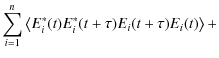
Using Eq. (6), we can show that (Loudon 2000, Eq. (3.7.13), p. 110), for n independent radiative atoms:
| = | 
|
||
|
|||
| (9) |
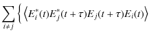
Only the terms where the field of a given atom is multiplied by its complex conjugates are kept. All other terms vanish because the average of the waves of the different atoms with random relative phases are zero; therefore,
| |
= | ||
In the usual case where
|
Using the definition of g(1) and g(2), we obtain Eq (1):
|
(10) |
Note that g(2) is a real number to the contrary of g(1). To recover the phase information, we can still use the amplitude itself thanks to the analycity of the discrete FT (see for instance Holmes & Belen'kii 2004, although an image flip degeneracy remains) or the high-order correlations (see for instance Zhilyaev 2008), but with the issue of even lower sensitivity.
The correlator of an intensity interferometer is designed to measure the quantity
![\begin{displaymath}\frac{\left\langle \left[ \bar{I}(\vec{r}, t) - \bar{I}~\righ...
...~\right] \right\rangle}{\bar{I}^2} = g^{(2)}(\vec{\rho}) - 1 ,
\end{displaymath}](/articles/aa/full_html/2009/45/aa11739-09/img34.png)
|
(11) |
where
| |
= | (12) | |
| = | (13) |
where it is assumed that the light source is stationary (i.e. its statistical properties does not change with time).
An intensity interferometer is schematized in Fig. 1
(right panel). In this case, path differences do not need to be
cancelled to the same precision, since the dominant fraction of this
path difference due to azimuthal distance and atmosphere fluctuations
is identical for both paths. However, the equality of both paths must
be achieved to a level corresponding to the difference of coherence
time between the two Fourier components:
![]() when
when
![]() .
This explains the less stringent need in high-precision optical devices
and the very poor sensitivity of the II against seeing fluctuations.
.
This explains the less stringent need in high-precision optical devices
and the very poor sensitivity of the II against seeing fluctuations.
2.4 The demonstration by Hanbury Brown of the working principle of the intensity interferometer
To clarify what an intensity interferometer measures and how it is related to the above formalism, let us briefly review the explanation provided by Hanbury Brown (Brown 1974, Chap. 2). The basic principle is schematized in Fig. 1 (right panel). Intensity interferometry is a second-order measurement, and instead of evaluating the electromagnetic fields in two different locations, it evaluates the correlations between pairs of point sources. Each points radiate white light and is completely independent of one another.
A lightwave can be decomposed as a superposition of a large number of
sinusoidal components, each component having a steady amplitude and
phase over the period of observation but both the amplitude and phase
being random with respect to the other components. Let us consider only
one component of this superposition (Hanbury Brown calls it a Fourier
component) reaching telescope A from P1 and another component with a different frequency reaching the same telescope A from the second point P2. We have
| (14) | |||
| (15) |
where E denotes the electromagnetic field amplitude of the given component.
The intensities are transformed into electrical currents in the
photodetectors. The output current as measured behind telescope A is proportional to the intensity of the light. Assuming linear polarization,
![\begin{displaymath}I_A = K_A \left[ E_1 \sin(\omega_1 t + \phi_1) + E_2 \sin(\omega_2 t + \phi_2)\right]^2
\end{displaymath}](/articles/aa/full_html/2009/45/aa11739-09/img46.png)
|
(16) |
where KA is a constant of the detector. The same Fourier component will also reach telescope B, with path differences d1 and d2; hence,
![$\displaystyle I_B = K_B [ E_1 \sin(\omega_1 (t + d_1/c) + \phi_1) +
E_2 \sin(\omega_2 (t + d_2/c) + \phi_2)]^2.$](/articles/aa/full_html/2009/45/aa11739-09/img47.png)
|
(17) |
If we expand these two equations, we obtain 4 terms each time. The first two terms are the sum of the light intensities from both components, and the third corresponds to the intensity of the sum of frequencies (
| IA | = | (18) | |
| IB | = | ||
| (19) |
These two components are correlated because they have the same beat frequency
![\begin{displaymath}c(d) = K_A K_B E_1^2 E_2^2 \cos\left[\frac{\omega}{c}(d_1-d_2)\right].
\end{displaymath}](/articles/aa/full_html/2009/45/aa11739-09/img56.png)
The phase difference between these correlated components is not the phase difference of the light waves at the two detectors but instead the difference between the phase differences (or the difference between the relative phases observed independently at the two telescopes) of the two Fourier components. By simple geometry, and because
![\begin{displaymath}c(d) = K_A K_B E_1^2 E_2^2 \cos\left[2\pi d \theta / \lambda\right]
\end{displaymath}](/articles/aa/full_html/2009/45/aa11739-09/img59.png)
|
(21) |
where d is the separation between the two telescopes. Finally, Brown & Twiss (1957) have shown that, when computing the total correlation by integrating Eq. (20) over all possible pairs of points on the disk of the star, over all possible pairs of Fourier components (which lie within the optical bandpass) and over all beat frequencies (which lie within the bandpass of the electrical filters), we obtain that the correlation is proportional to the square of the modulus of the visibility.
Clearly, by no means in this analysis is the hypothesis of chaotic light explicitly made. It nonetheless plays an important role.
2.5 The implicit hypothesis of the chaotic nature of light in the Narrabri stellar intensity interferometer experiment
As said in the introduction, Brown & Twiss (1957) never hypothesized that the light source must be producing chaotic light. We use here the term ``chaotic'' instead of ``thermal'', since chaotic light can be produced by independent nonthermal individual sources. The subtle distinction is important in the case of radio masers, as discussed below.
It is interesting to note that the year 1957 is also the time when lasers developed (e.g. Schawlow & Townes 1958), and their properties were probably not fully known and understood at that time. In their paper of 1957, Hanbury Brown and Twiss even claim that the effect of correlation between intensity fluctuations had nothing to do with the mechanism by which the light was actually produced. They end their paper by saying: ``[...] still less does it imply that the photons must have been injected coherently into the radiation field. On the contrary, if one wishes to picture the electromagnetic field as a stream a photons, one has to imagine that the light quanta redistribute themselves over the wavefront, as the radiation field, which may be quite incoherent in origin, is focused and collimated into beams capable of mutual interference; thus the correlation between photons is determined solely by the energy distribution and coherence of the light reaching the photon detectors''.
Interestingly, Hanbury Brown make no reference to the nature of light itself when presenting the above analysis based on Fourier components, noting that this way is ``freer from conceptual traps''. However, in his book in 1974 he presented the analysis in a slightly different manner, although not emphasizing the radical difference it implies for interpreting of the phenomenon. At the beginning of Chap. 3, he did start by stating that ``white light of the thermal origin has the properties of a Gaussian random process'' as shown by several classical papers. This property is used further in his analysis but never to express how the results could have been different in the case of nonthermal light. In the formalism presented above, it lies precisely at the point where we identify Eqs. (6) and (7).
It is known today, however, that photons may follow different
statistics and that it depends precisely on how the collections of
photons are emitted. This does not invalidate the analysis presented
above, but it does prevent interpreting the correlation seen in g(2) as a measurement of the visibility
![]() ,
hence as information about the angular distribution of light intensity
along a baseline separating two telescopes via the classical van
Cittert-Zernike theorem. In other words, Eq. (1)
is not satisfied for non-chaotic light. For instance, it can be shown
that, for an ideal monochromatic linearly-polarized laser, we have
,
hence as information about the angular distribution of light intensity
along a baseline separating two telescopes via the classical van
Cittert-Zernike theorem. In other words, Eq. (1)
is not satisfied for non-chaotic light. For instance, it can be shown
that, for an ideal monochromatic linearly-polarized laser, we have
![]() ,
independent of
,
independent of ![]() .
It also means that no additional information at all is encoded in
higher order functions in chaotic light. In fact, one can show that for
this type of light alone, it is always possible to write the nth order of the correlation function as sums of products of the first-order function (Glauber 2007, p. 115).
.
It also means that no additional information at all is encoded in
higher order functions in chaotic light. In fact, one can show that for
this type of light alone, it is always possible to write the nth order of the correlation function as sums of products of the first-order function (Glauber 2007, p. 115).
2.6 Photon statistics and non-classical light
Interestingly, different types of light can be classified thanks to g(2)![]() ), or more precisely, they depend on their value of g(2)
), or more precisely, they depend on their value of g(2)
![]() .
A typical experimental setup to measure g(2)
.
A typical experimental setup to measure g(2)![]() is sketched in Fig. 2.
A counter is started when a photon is detected on A and run until
another photon is detected on B, which causes the counter to stop. With
time accumulating, a histogram of events can be gradually built as a
function of the duration during which the counter ran. By counting the
number of events as a function of the time difference
is sketched in Fig. 2.
A counter is started when a photon is detected on A and run until
another photon is detected on B, which causes the counter to stop. With
time accumulating, a histogram of events can be gradually built as a
function of the duration during which the counter ran. By counting the
number of events as a function of the time difference ![]() ,
we measure g(2)
,
we measure g(2)![]() .
Typical results are illustrated in Fig. 3. In the case of a intensity interferometer, the beam splitter is replaced by the spatial extent of the light source.
.
Typical results are illustrated in Fig. 3. In the case of a intensity interferometer, the beam splitter is replaced by the spatial extent of the light source.
![\begin{figure}
\par\includegraphics[angle=-90,width=9cm]{11739f2.eps}
\end{figure}](/articles/aa/full_html/2009/45/aa11739-09/img65.png)
|
Figure 2: Sketch of a typical experimental setup to measure g(2). Light or photons come from the left and enter the 50:50 beamsplitter. If a photon is detected on detector A, a counter is started. This counter runs until another photon is recorded in Detector B (see Fox 2006). It basically corresponds to the Narrabri interferometer setup, if the beam splitter is replaced by two telescopes recording an intensity each. The principle, however, remains the same. |
| Open with DEXTER | |
![\begin{figure}
\par\includegraphics[width=8cm]{11739f3.eps}
\end{figure}](/articles/aa/full_html/2009/45/aa11739-09/img66.png)
|
Figure 3:
Example of g(2) curves for light of coherence time
|
| Open with DEXTER | |
Quantum optics experiments have shown that g(2)(0)
can be smaller than unity, which is the signature of non-classical
light. To compare this result to the classical light fluctuations, we
adopt a quantum description in terms of photons. Intensity fluctuations
can be understood as ``bunches'' of photons; in other words, in chaotic
light, photons tends to arrive in groups because the collection of
individual photon emission is randomly disturbed (by, for instance,
collisions between atoms in the emitting plasma). These bunches are
characterized by a distribution of arrival times that is super
Poissonian, i.e. with a statistical variance following:
![]()
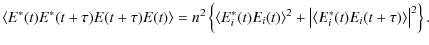
Similarly, in the section of the light beam of an ideal monochromatic
polarized laser, the arrival time of a photon will not be correlated at
all with that of any other one, g(2)![]() remains equal to unity whatever the value of
remains equal to unity whatever the value of ![]() ,
and the variance is perfectly Poissonian:
,
and the variance is perfectly Poissonian:
![]() .
From a classical point of view, the intensity of such laser has no fluctuations at all and an infinite coherence time.
.
From a classical point of view, the intensity of such laser has no fluctuations at all and an infinite coherence time.
The case of g(2)(0) < 1 is often called
anti-bunching. This cannot be interpreted in a classical sense (the
light would have a coherence time longer than that of a laser, i.e.
larger than infinity) and need a quantum description. To be exact,
anti-bunching and sub-poissonian statistics are not exactly the same
(see e.g. Zou & Mandel 1990; Singh 1983),
even if they tend to be satisfied simultaneously. Formally,
anti-bunched light is light whose degree of second-order coherence
satisfies g(2)![]() g(2)(0), while light with sub-Poissonian statistics satisfies g(2)(0) < 1 (see also Loudon 2000, Chap. 6.5).
g(2)(0), while light with sub-Poissonian statistics satisfies g(2)(0) < 1 (see also Loudon 2000, Chap. 6.5).
Photon anti-bunching is only one aspect of the quantum properties of light among many others: squeezed states, intricated photons, slow light, and so on. It is, however, the first observable that could be used in astrophysics requiring only a large photon collector, and ultra-fast, efficient detectors. It is beyond the scope of this paper to see whether other properties can be studied in practice in an astrophysical context. At this stage, we focus on light statistics and anti-bunching, which still represents truly unknown territory in optical observations of astrophysical sources.
3 The intensity interferometer: fundamental limitations and new detectors
In other places have been presented some considerations about using present and future Cerenkov telescope arrays to build a modern intensity interferometer (see in particular LeBohec & Holder 2005; Ofir & Ribak 2006b; de Wit et al. 2008b). It is already known that one of the main issues with II is its much lower sensitivity compared to an amplitude interferometer, since a second-order effect is measured. On the other hand, it is often believed that, by improving the various parts of the original II experiment and multiplying the number of baselines/telescopes, one can build a modern interferometer that could open the window towards new scientific results. Although it may certainly be true in practice, we show below that there are at least two fundamental limitations that do not exist with a phase interferometer and that must be kept in mind when looking for science applications for an II.
3.1 It works for chaotic light only
We have explained above why an II ultimately relies on the chaotic nature of the light produced by the source to measure of stellar radii. This hypothesis of chaotic light is certainly verified in the case of thermal light, where the emission processes are dominated by random collisions and Doppler broadening. As a result, a modern intensity interferometer will remain (only) an imaging device of thermal sources.
Interestingly, second-order coherence has been looked for in radio masers, but no deviation from a super-Poissonian statistics has been found (Moran 1981; Evans et al. 1972). The only interpretation proposed is that, even though a maser produce locally coherent light, an astrophysical object called ``maser'' is made of a collection of individual coherent sources that have random motions relative to each other.
This example illustrates the obvious fact that the interpretation of photon statistics in an astrophysical observation is not necessarily straightforward and requires some a priori knowledge of the source.
3.2 The hotter, the better
The second fundamental limitation of an II is that the amount
of intensity fluctuations, i.e. the ``signal'' used to measure stellar
radii, decreases rapidly with the star's surface temperature. In other
words, the hotter, the better. For a thermal source, the photon
statistics follows the Bose-Einstein distribution, whose variance
writes as

|
(22) |
The first term, called the shot noise, originates from the discrete nature of light (photons), while the second, called wave noise, truly represents the fluctuations of the energy of the electromagnetic radiation, so this term is the ``signal''. However, its contribution to the total noise is rather small at optical frequencies.
Following Goodman (1985, Eqs. (9.3-8) and (9.5-19)),
assuming that individual count-products at the output of the device for
a single counting interval are independent of one interval to another,
the S/N writes for a blackbody as
|
(23) |
where V is the first-order visibility,
|
(24) |
where T is the source's temperature (see Goodman 1985, Chap. 9.5). We note that wave noise is by far the dominant source of noise in the radio-frequency domain.
For a given S/N ratio, visibility and integration interval, we computed the exposure times as a function of the star's temperature, and normalized it by solar values. The result is shown in Fig. 4. One can clearly see that, compared to the observation of a solar analog, cooler stars rapidly require much longer exposure times, especially at short wavelengths, while it is not as critical when observing at infrared wavelengths. This limitation illustrates that Hanbury Brown & Twiss observed mostly hot stars, and it must be taken into account when looking for scientific application of a modern II.
![\begin{figure}
\par\includegraphics[width=8.8cm]{11739f4.eps}
\end{figure}](/articles/aa/full_html/2009/45/aa11739-09/img79.png)
|
Figure 4:
Exposure time required to observe a given S/N
ratio with a given visibility and detector integration interval, as a
function of the stellar temperature, normalized to solar values. The
blue solid curve shows the case for visible light (
|
| Open with DEXTER | |
3.3 New photon-counting HgCdTe Avalanche Photodiodes and the quantum limit
The intensity interferometry is the measurement of a second-order
effect and, as such, is poorly sensitive. This limitation explains the
need for large light collectors, hence the concomitant interest in this
technique with the future advent of very large optical telescopes. On
the other hand, another component that is not less critical are the
detectors. More efficient and rapid detectors slightly relieve the
requirements on the mirror's size, although they increase the
requirement for isochronicity of the mirrors. As matter of fact, they
are central when looking for light statistics, since the quantum
efficiency measures the fidelity of this statistics. Using a
semi-classical approach for photodetection, one can show (e.g. Fox 2006) that the observed variance of the statistics of photon arrival times writes as
|
(25) |
where the quantum efficiency
The other obvious parameter to consider is the shortest time interval
accessible by the detector, or inversely its bandwidth. It can be shown
that, for instance in the case of chaotic light, the observed photon statistics variance writes as
|
(26) |
where
Detectors considered by the time of QuantEYE prospective work (a concept of photon-counting instrument for the E-ELT, see Dravins et al. 2005, and below) were limited to the nanosecond accuracy. However, new perspectives could be opened by a novel type of polarized HgCdTe Avalanche Photodiodes developed at the Commissariat à l'Energie Atomique (CEA) in Grenoble (Rothman et al. 2008). It appears that these diodes could have a high gain, a low dark current, a very high quantum efficiency (above 95%) and will detect single photons in the optical-near infrared domain with an accuracy of time tagging better than 100 picoseconds (Rothman, private communication).
![\begin{figure}
\par\includegraphics[width=8.8cm]{11739f5.eps}
\end{figure}](/articles/aa/full_html/2009/45/aa11739-09/img90.png)
|
Figure 5:
Impact of the new APDs on the limiting magnitude of an II. The comparison is made with LeBohec & Holder (2005), using a minimal S/N of 3, and a 10-h night integration, an overall reflectivity of R=0.6, which gives a limiting magnitude of about 8 for a telescope area of
|
| Open with DEXTER | |
Fundamentally speaking, one can define an observational
``photon-counting quantum limit'' by using Heisenberg's uncertainty
principle:
| (27) |
Using the expected accuracy of the detectors above (80 picoseconds) and a central wavelength of
One can evaluate the impact of such detectors by using a formula of Brown (1974, see Eq. (4.30), p. 50) taking the telescope size and the overall quantum efficiency of the system into account:

|
(28) |
where A is the telescope area in square meters,
We emphasize that these estimations are somehow optimistic. Brown (1974) observed true S/N systematically lower by 25% compared to his theoretical calculations given by the above formula. He gave no explanations, but identified the most probable cause of this discrepancy as the cumulative result of several small errors in various parameters: overall loss of the optical system, the excess noise, and atmospheric effects.
4 New scientific questions
A revival of the intensity interferometry is interesting because it may create, among other things, new means of performing high-resolution angular imaging (de Wit et al. 2008b). However, in our opinion, this return of interest could be broader and should encompass the perspectives already outlined in the prospective work of the photon-counting instrument QuantEYE (Dravins et al. 2005) proposed for the E-ELT (D'Odorico 2005, at that time the ELT was called OWL and was expected to have a 100 m primary mirror), to which the reader is referred for a broad review of observational high-speed astrophysics. In that context, one must explore the new possibilities offered by true photon-counting devices. We note that some experiments have already started at the Asagio observatory (AquaEYE; Barbieri et al. 2007; Naletto et al. 2007).
With truly new possibilities, we think it is important to explore new questions, which go beyond what is accessible by the current (or even foreseen) ``classical'' observational techniques. In this section we attempt to contribute to these efforts by presenting why microquasars in our galaxy, and possibly their extragalactic equivalent the quasars, could represent an excellent first target in the optical/near-infrared for observing nonthermal light and testing the use of g(2) in astrophysical sources.
We note that Hanbury Brown judged it unlikely that the coincidence-counting interferometry was of any interest for astrophysics. The reason he gives (end of Chap. 4) is essentially technical and related to the bandwidth having to be limited not to saturate the detector and to permit counting each single photon. The example he took is, however, that of a zero-th magnitude star.
4.1 Microquasars under the quantum microscope
Microquasars are short-period X-ray binaries with one of its components a stellar-mass black-hole. These objects are the closest relativistic objects to us. They sometimes show superluminal jets (e.g. Mirabel & Rodriguez 1994) and produce copious amounts of X-rays. Powerful and self-collimated jets are produced in the inner regions of the accretion disk (e.g. Ferreira et al. 2006). Microquasars share the same physics as quasars and probably gamma-ray bursts (since they share the same physical ingredients: a black-hole, an accretion disk and jets) so they must be understood in the same framework (Mirabel 2004). Microquasars are nowadays studied mostly in X-rays because it is where the physics of the closest regions around the black hole can be probed.
Interestingly, the jets in microquasars are supersonic, which means that the particles emitting synchrotron radiation are moving faster than the local perturbations, possibly avoiding the problem observed in radio masers. Moreover, the jets are being produced very close to the central black hole. Therefore, jets could possibly be used to probe the region around the black hole similar to what is made nowadays: the accretion disk and its oscillations (called quasi-periodic oscillation - QPOs, see for instance van der Klis 2005) can be used to estimate black-hole spin (Remillard & McClintock 2006).
The optical/near-infrared region of the spectrum is well-suited to
studying the interface between the jets and the accretion disk around
the black hole. Figure 6 illustrates a typical theoretical spectral energy distribution (SED) of a microquasar with a black-hole mass of 10 ![]() at a distance of 10 kpc (see e.g. Foellmi et al. 2008a, Foellmi et al. 2009, in prep.). The left panel shows the observed flux of the various radiating components in erg s-1 cm-2.
The most central regions of the accretion disk around the black hole
produce the strong X-ray emission. However, the same SED expressed in
terms of photons (right panel) shows a completely different situation.
In the far-UV and X-ray domains, there is simply too few photons for
statistical studies.
at a distance of 10 kpc (see e.g. Foellmi et al. 2008a, Foellmi et al. 2009, in prep.). The left panel shows the observed flux of the various radiating components in erg s-1 cm-2.
The most central regions of the accretion disk around the black hole
produce the strong X-ray emission. However, the same SED expressed in
terms of photons (right panel) shows a completely different situation.
In the far-UV and X-ray domains, there is simply too few photons for
statistical studies.
![\begin{figure}
\par\mbox{\includegraphics[width=4.4cm]{11739f6a.eps}\hspace*{1.5mm}
\includegraphics[width=4.4cm]{11739f6b.eps} }\end{figure}](/articles/aa/full_html/2009/45/aa11739-09/img97.png)
|
Figure 6:
Theoretical spectral energy distributions of a microquasar as a function of the frequency |
| Open with DEXTER | |
Finally, let us mention an example of another quantum property of the light produced, in theory, near a black hole: the Unruh process (a cinematic version of the Hawking radiation, Unruh 1976) is expected to produce pairs of photons with maximally entangled polarizations (Schützhold et al. 2006).
5 Summary and conclusions
In this research note, we have presented the mathematical basics about the first and the second order correlation functions, and discussed them in the context of astronomical observations.
It appears fairly clear that detailed physical and quantitative predictions of quantum phenomena in astrophysical sources accessible with photon-counting devices are still lacking. In the context of the development of large Cerenkov arrays and future Extremely Large Telescopes, we think that these questions deserve more dedicated studies.
AcknowledgementsC.F. thanks E. Le Coarer, J. Rothman, D. Dravins, P. Kern, G. Duvert, D. Mouillet, S. Maret, and A. Chelli for exciting discussions, J.-P. Berger for providing a very useful reference, and K. Schuster for encouragements. C.F. also acknowledges support from the Swiss National Science Foundation (grant PA002-115328).
References
- Alexander, G. 2003, Rep. Prog. Phys., 66, 481 [NASA ADS] [CrossRef]
- Barbieri, C., Naletto, G., Occhipinti, T., et al. 2007, Mem. S. A. It. Supp., 11, 190
- Baym, G. 1998, Acta Phys. Polon. B, 29, 1839 [NASA ADS]
- Borra, E. F. 2008, MNRAS, 389, 364 [NASA ADS] [CrossRef]
- Brown, R. H. 1974 (New York: Halsted Press)
- Brown, R. H., & Twiss, R. Q. 1957, Proc. R. Soc. London Ser. A, 242, 300 [NASA ADS] [CrossRef]
- Brown, R. H., & Twiss, R. Q. 1958a, Proc. R. Soc. London Ser. A, 243, 291 [NASA ADS] [CrossRef]
- Brown, R. H., & Twiss, R. Q. 1958b, Proc. R. Soc. London Ser. A, 248, 199 [NASA ADS] [CrossRef]
- Brown, R. H., & Twiss, R. Q. 1958c, Proc. R. Soc. London Ser. A, 248, 222 [NASA ADS] [CrossRef]
- de Wit, W. J., Bohec, S. L., Hinton, J. A., et al. 2008a, High Time Resolution Astrophysics: The Universe at Sub-Second Timescales. AIP Conf. Proc., 984, 268 [NASA ADS]
- de Wit, W. J., LeBohec, S., Hinton, J. A., et al. 2008b, J. Phys.: Conf. Ser., 131, 2050 [NASA ADS]
- D'Odorico, S. 2005, The Messenger (ESO), 122, 6 [NASA ADS], (c) 2005: European Southern Observatory
- Dravins, D. 2008, High Time Resolution Astrophysics, Astrophys. Space Sci. Libr. (Springer), 351, 95
- Dravins, D., Barbieri, C., Fosbury, R. A. E., et al. 2005, Proceedings of Instrumentation for Extremely Large Telescopes [arXiv:astro-ph/0511027]
- Evans, N., Rydbeck, O. E. H., & Kollberg, E. 1972, Phys. Rev. A, 6, 1643 [NASA ADS] [CrossRef]
- Ferreira, J., Petrucci, P.-O., Henri, G., Saugé, L., & Pelletier, G. 2006, A&A, 447, 813 [NASA ADS] [CrossRef] [EDP Sciences]
- Foellmi, C., Petrucci, P. O., Ferreira, J., et al. 2008a, Proceedings of The Microquasar Workshop #7 [arXiv:0810.0108]
- Foellmi, C., Petrucci, P.-O., Ferreira, J., Henri, G., & Boutelier, T. 2008b, SF2A-2008: Proc. of the Annual meeting of the French Society of Astronomy and Astrophysics, ed. C. Charbonnel, 211
- Fox, M. 2006, Quantum Optics: An Introduction (Oxford University Press)
- Glauber, R. J. 2007, Quantum Theory of Optical Coherence: Selected Papers and Lectures (Wiley-VCH), 639
- Goodman, J. W. 1985, Statistical Optics, Wiley
- Haniff, C. 2007, New Astron. Rev., 51, 565 [NASA ADS] [CrossRef]
- Holmes, R. B., & Belen'kii, M. S. 2004, J. Opt. Soc. Amer. A, 21, 697 [NASA ADS] [CrossRef]
- Jain, P., & Ralston, J. P. 2008, A&A, 484, 887 [NASA ADS] [CrossRef] [EDP Sciences]
- LeBohec, S., Barbieri, C., Wit, W.-J. D., et al. 2008, Proc. of the SPIE, 7013, 70132E
- LeBohec, S., & Holder, J. 2005, 29th International Cosmic Ray Conference [arXiv:astro-ph/0507010]
- Loudon, R. 2000, The Quantum Theory of Light (Oxford University Press)
- Mirabel, I. F. 2004, Proceedings of the 5th INTEGRAL Workshop on the INTEGRAL Universe (ESA SP-552), 16-20 February, 552, 175
- Mirabel, I. F., & Rodriguez, L. F. 1994, Nature, 371, 46 [NASA ADS] [CrossRef]
- Moran, J. M. 1981, BAAS, 13, 508 [NASA ADS]
- Naletto, G., Barbieri, C., Occhipinti, T., et al. 2007, Proc. SPIE, 6583, 9 [NASA ADS]
- Ofir, A., & Ribak, E. N. 2006a, MNRAS, 368, 1646 [NASA ADS] [CrossRef]
- Ofir, A., & Ribak, E. N. 2006b, MNRAS, 368, 1652 [NASA ADS] [CrossRef]
- Remillard, R. A., & McClintock, J. E. 2006, ARA&A, 44, 49 [NASA ADS] [CrossRef]
- Rothman, J., Perrais, G., Ballet, P., et al. 2008, J. Electron. Mater., 37, 1303 [NASA ADS] [CrossRef]
- Schawlow, A. L., & Townes, C. H. 1958, Phys. Rev., 112, 1940 [NASA ADS] [CrossRef]
- Schützhold, R., Schaller, G., & Habs, D. 2006, Phys. Rev. Let., 97
- Singh, S. 1983, Optics Communications, 44, 254 [NASA ADS] [CrossRef]
- Unruh, W. G. 1976, Phys. Rev. D, 14, 870 [NASA ADS] [CrossRef]
- van der Klis, M. 2005, Astron. Nachr., 326, 798 [NASA ADS] [CrossRef]
- Zhilyaev, B. E. 2008, Contribution to the SPIE meeting in Marseille: Digital revival of intensity interferometry with atmospheric Cherenkov Telescope arrays [arXiv:0806.0191]
- Zou, X. T., & Mandel, L. 1990, Phys. Rev. A, 41, 475 [NASA ADS] [CrossRef]
Footnotes
- ... interferometry
![[*]](/icons/foot_motif.png)
- An interest strong enough for the International Astronomical Union to create a dedicated Working Group.
- ... respectively
- Parenthesis indicate that the number is not an exponent.
- ... NSII
- Strictly speaking, the NSII was preceded by two experiments of the same nature, performed in Jodrell Bank (England) led by Hanbury Brown. The first one was operating in the radio frequencies and was used to measure the angular diameter of the Sun and to study Cassiopeia A and Cygnus A. The second one was a crude optical II dedicated to proving the feasibility of the concept by measuring the angular diameter of Sirius. See Brown (1974) for the details and subsequent references. Historically, the NSII remains, however, the true experiment demonstrating the correlations of intensity fluctuations.
All Figures
|
|
Figure 1: Working principle of an intensity interferometer compared to that of a Michelson interferometer. On the left (Michelson interferometer), a first-order spatial coherence measurement is made, associated with the statistical average of single point sources. Delay lines are used to cancel out the path difference d1 and ensure temporal coherence. On the right (intensity interferometer), a second-order spatial coherence measurement is made, associated with the statistical average of the correlations between pairs of point sources. |
| Open with DEXTER | |
| In the text | |
|
|
Figure 2: Sketch of a typical experimental setup to measure g(2). Light or photons come from the left and enter the 50:50 beamsplitter. If a photon is detected on detector A, a counter is started. This counter runs until another photon is recorded in Detector B (see Fox 2006). It basically corresponds to the Narrabri interferometer setup, if the beam splitter is replaced by two telescopes recording an intensity each. The principle, however, remains the same. |
| Open with DEXTER | |
| In the text | |
|
|
Figure 3:
Example of g(2) curves for light of coherence time
|
| Open with DEXTER | |
| In the text | |
|
|
Figure 4:
Exposure time required to observe a given S/N
ratio with a given visibility and detector integration interval, as a
function of the stellar temperature, normalized to solar values. The
blue solid curve shows the case for visible light (
|
| Open with DEXTER | |
| In the text | |
|
|
Figure 5:
Impact of the new APDs on the limiting magnitude of an II. The comparison is made with LeBohec & Holder (2005), using a minimal S/N of 3, and a 10-h night integration, an overall reflectivity of R=0.6, which gives a limiting magnitude of about 8 for a telescope area of
|
| Open with DEXTER | |
| In the text | |
|
|
Figure 6:
Theoretical spectral energy distributions of a microquasar as a function of the frequency |
| Open with DEXTER | |
| In the text | |
Copyright ESO 2009
Current usage metrics show cumulative count of Article Views (full-text article views including HTML views, PDF and ePub downloads, according to the available data) and Abstracts Views on Vision4Press platform.
Data correspond to usage on the plateform after 2015. The current usage metrics is available 48-96 hours after online publication and is updated daily on week days.
Initial download of the metrics may take a while.