| Issue |
A&A
Volume 507, Number 2, November IV 2009
|
|
|---|---|---|
| Page(s) | 995 - 1004 | |
| Section | The Sun | |
| DOI | https://doi.org/10.1051/0004-6361/200912930 | |
| Published online | 15 September 2009 | |
A&A 507, 995-1004 (2009)
On the emergence of toroidal flux tubes: general dynamics and comparisons with the cylinder model
D. MacTaggart - A. W. Hood
School of Mathematics and Statistics, University of St Andrews, North Haugh, St Andrews, Fife, KY16 9SS, Scotland
Received 20 July 2009 / Accepted 9 September 2009
Abstract
Aims. In this paper we study the dynamics of toroidal flux
tubes emerging from the solar interior, through the photosphere and
into the corona. Many previous theoretical studies of flux emergence
use a twisted cylindrical tube in the solar interior as the initial
condition. Important insights can be gained from this model, however,
it does have shortcomings. The axis of the tube never fully emerges as
dense plasma becomes trapped in magnetic dips and restrains its ascent.
Also, since the entire tube is buoyant, the main photospheric
footpoints (sunspots) continually drift apart. These problems make it
difficult to produce a convincing sunspot pair. We aim to address these
problems by considering a different initial condition, namely a
toroidal flux tube.
Methods. We perform numerical experiments and solve the 3D MHD
equations. The dynamics are investigated through a range of initial
field strengths and twists.
Results. The experiments demonstrate that the emergence of
toroidal flux tubes is highly dynamic and exhibits a rich variety of
behaviour. In answer to the aims, however, if the initial field
strength is strong enough, the axis of the tube can fully emerge. Also,
the sunspot pair does not continually drift apart. Instead, its maximum
separation is the diameter of the original toroidal tube.
Key words: Sun: magnetic fields - magnetohydrodynamics - methods: numerical
1 Introduction
It is generally accepted that solar active regions, and therefore
sunspots, are the result of magnetic flux tubes that have risen from
the base of the convection zone and emerged at the photosphere. The
emerging flux tubes are ![]() -shaped,
at least near photosphere, and produce bipolar sunspot pairs. This has
been the classical picture of sunspot formation for some time. Cowling (1946)
envisaged flux tubes running as girdles around the Sun and suggested
that loops were carried upwards by convection to emerge as sunspot
pairs. Soon after, the idea of magnetic buoyancy was put forward as the mechanism by which flux tubes journey from the base of the convection zone to the photosphere (Parker 1955; Jensen 1955).
Parker demonstrated that an isolated magnetic flux tube in a stratified
plasma under gravity must be buoyant, provided that it is close to
thermal equilibrium with its surroundings. Although the exact mechanism
by which flux tubes rise in the convection zone is not known, most
theorists tend to favour magnetic buoyancy. Simulations using spherical
geometry have now been performed which show how a twisted flux tube can
survive rising buoyantly though the convection zone (Jouve & Brun 2007; Fan 2008).
-shaped,
at least near photosphere, and produce bipolar sunspot pairs. This has
been the classical picture of sunspot formation for some time. Cowling (1946)
envisaged flux tubes running as girdles around the Sun and suggested
that loops were carried upwards by convection to emerge as sunspot
pairs. Soon after, the idea of magnetic buoyancy was put forward as the mechanism by which flux tubes journey from the base of the convection zone to the photosphere (Parker 1955; Jensen 1955).
Parker demonstrated that an isolated magnetic flux tube in a stratified
plasma under gravity must be buoyant, provided that it is close to
thermal equilibrium with its surroundings. Although the exact mechanism
by which flux tubes rise in the convection zone is not known, most
theorists tend to favour magnetic buoyancy. Simulations using spherical
geometry have now been performed which show how a twisted flux tube can
survive rising buoyantly though the convection zone (Jouve & Brun 2007; Fan 2008).
Due to the wide variety of phenomena that exist in sunspots, different
modelling techniques have been developed to describe them. These range
from equilibrium models (e.g. Petrie & Neukirch 1999) to studies of magnetoconvection (e.g. Heinemann et al. 2007). A useful collection of these methods, and general sunspot physics, is presented in Thomas & Weiss (2008,1992).
In recent years it has become possible to simulate the rise of flux
tubes in the upper convection zone and their emergence into the
atmosphere. The first 3D simulation of the emergence of a twisted flux
tube in a stratified atmosphere was performed by Fan (2001). Several similar simulations have been performed since and are described in a recent review by Archontis (2008).
What all of these types of flux emergence simulations have in common is
that they use the same initial condition, namely a cylindrical twisted
flux tube in the solar interior. To encourage the formation of an ![]() -shaped loop, a density deficit is introduced into the tube that is proportional to
-shaped loop, a density deficit is introduced into the tube that is proportional to
![]() ,
where y is the horizontal coordinate along the tube length and
,
where y is the horizontal coordinate along the tube length and ![]() is a parameter describing the length of the buoyant section of the tube. When the
is a parameter describing the length of the buoyant section of the tube. When the ![]() -loop
emerges it creates a sunspot pair at the photosphere. Much has been
gained from this model, however, it contains some drawbacks. The
cylindrical tube continues to emerge and the sunspot pair continually
drifts apart. This is not seen in observations, where active regions
spread to a finite size and then decay (Liu & Zhang 2006).
Another drawback is that, in simulations with this initial condition,
the original axis of the tube remains trapped at the base of the
photosphere and never emerges to be almost vertical when it leaves and
enters the sunspots. In this paper we consider a different geometry for
initial the magnetic field - a toroidal flux tube. This model was originally considered by Hood et al. (2009).
We shall investigate the behaviour of emerging toroidal tubes through a
range of initial field strengths and twists. Our approach is to
consider an idealized stratified solar interior and atmosphere. We are
interested in the interaction of the plasma and the magnetic field, so
we solve the 3D resistive and compressive magnetohydrodynamic (MHD)
equations. The aim is, using the toroidal model, to answer the
following questions:
-loop
emerges it creates a sunspot pair at the photosphere. Much has been
gained from this model, however, it contains some drawbacks. The
cylindrical tube continues to emerge and the sunspot pair continually
drifts apart. This is not seen in observations, where active regions
spread to a finite size and then decay (Liu & Zhang 2006).
Another drawback is that, in simulations with this initial condition,
the original axis of the tube remains trapped at the base of the
photosphere and never emerges to be almost vertical when it leaves and
enters the sunspots. In this paper we consider a different geometry for
initial the magnetic field - a toroidal flux tube. This model was originally considered by Hood et al. (2009).
We shall investigate the behaviour of emerging toroidal tubes through a
range of initial field strengths and twists. Our approach is to
consider an idealized stratified solar interior and atmosphere. We are
interested in the interaction of the plasma and the magnetic field, so
we solve the 3D resistive and compressive magnetohydrodynamic (MHD)
equations. The aim is, using the toroidal model, to answer the
following questions:
- 1.
- can the axis of the original flux tube emerge into the solar atmosphere and, if so, how?
- 2.
- can the two main polarities of the active region (sunspots) drift to a fixed distance and then stop?
2 Model setup
In this section we outline the numerical setup and the initial atmosphere and magnetic field configurations.2.1 Main equations
For our numerical experiments we use a 3D version of the Lagrangian remap scheme detailed in Arber et al. (2001). This code has been used for other flux emergence studies (Archontis & Török 2008; Archontis et al. 2009).
For each time step, the equations are solved in Lagrangian form and are
then remapped back onto an Eulerian grid. All of the physics is
contained in the Lagrangian step. The variables are made dimensionless
against photospheric values. These values are: pressure,
![]() ;
density,
;
density,
![]() ;
temperature,
;
temperature,
![]() and scale height
and scale height
![]() .
The other units used in the simulations are: time,
.
The other units used in the simulations are: time,
![]() ;
speed,
;
speed,
![]() and magnetic field
and magnetic field
![]() .
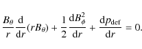
The evolution of the system is governed by the following time-dependent and resistive (non-dimensionalized) MHD equations:
.
The evolution of the system is governed by the following time-dependent and resistive (non-dimensionalized) MHD equations:
|
(1) |
|
(2) |

|
(3) |
|
(4) |
with specific energy density

The basic variables are the density
where
2.2 Initial atmosphere
The initial stratification of the atmosphere is similar to that used in previous flux emergence studies (Fan 2001; MacTaggart & Hood 2009; Murray et al. 2006). The solar interior ![]() is taken to be marginally stable to convection since in this study we
are focussing on the emerging field. The effects of convection are left
for future work. The photosphere/chromosphere lies in the region
is taken to be marginally stable to convection since in this study we
are focussing on the emerging field. The effects of convection are left
for future work. The photosphere/chromosphere lies in the region
![]() ,
the transition region in
,
the transition region in
![]() and the corona in
and the corona in ![]() .
The (non-dimensionalized) temperature is specified as
.
The (non-dimensionalized) temperature is specified as
where
2.3 Initial magnetic field
As mentioned earlier, nearly all previous studies of numerical flux emergence use a twisted cylindrical flux tube in the solar interior as the initial condition. Here we present the cylinder and the toroidal models.
2.3.1 Cylinder model
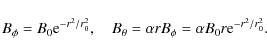
The magnetic field of a twisted cylindrical flux tube (Fan 2001) is given by
where
The pressure inside the tube differs from the surrounding field-free region by
![]() .
Balancing the radial components of the Lorentz force and the plasma pressure gradient gives
.
Balancing the radial components of the Lorentz force and the plasma pressure gradient gives
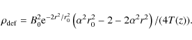
Solving this gives a pressure deficit, relative to the background hydrostatic pressure, of
|
(10) |
The density deficit can then be calculated from
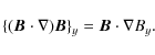
2.3.2 Toroidal model
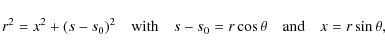
A full derivation of this model is given in Hood et al. (2009) so we shall only outline certain steps here. If, in Cartesian coordinates, the tube axis lies in the y-direction then the equations for the magnetic field can be written in polar coordinates
![]() :
:
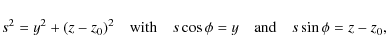
where z0 is the base of the computational box. Under the assumption of rotational invariance, we take the magnetic field to be of the form
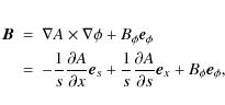
where A is the flux function and is constant on magnetic field lines. This form automatically satisfies the solenoidal constraint, Eq. (5). After some manipulation, insertion of this field into the magnetostatic balance equation,
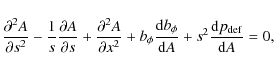
where
with major axis s0. Rewriting Eq. (11) in these local coordinates and then taking a regular expansion in the aspect ratio r0/s0 produces the leading order balance equation
This has the same form as Eq. (9) from the cylinder model. We can, therefore, choose the solutions to be the same as those for the straight tube. These are, as in (7) and (8),
Again, B0 is the axial field strength and
In the simulations the entire toroidal tube is made buoyant. We could find more terms in the expansion but since we do not require an exact equilibrium (as the tube will be made buoyant) we only consider the leading order solution.
The resulting magnetic field for a twisted toroidal tube is given (in Cartesian coordinates) by
| Bx | = | (13) | |
| By | = | (14) | |
| Bz | = | (15) |
3 Parameter study
Now that the basic model is established, we shall investigate the
dynamics of toroidal flux emergence by considering a range of
parameters. In this study we look at the effects of changing the
initial field strength B0 and the initial twist ![]() .
The other parameters will be kept constant in this paper: s0=15, r0=2.5 and z0=-25.
.
The other parameters will be kept constant in this paper: s0=15, r0=2.5 and z0=-25.
3.1 Varying B0 with fixed  :
general dynamics
:
general dynamics
In this section we consider the effects of changing the initial field strength, B0, and keep the initial twist fixed at
![]() .
This value is smaller than those used in previous studies (Archontis & Török 2008; Fan 2001; Hood et al. 2009; Murray et al. 2006) and is believed to be more applicable to the Sun. We follow the evolution for the cases
B0 = 1,3,5,7 and 9.
.
This value is smaller than those used in previous studies (Archontis & Török 2008; Fan 2001; Hood et al. 2009; Murray et al. 2006) and is believed to be more applicable to the Sun. We follow the evolution for the cases
B0 = 1,3,5,7 and 9.
![\begin{figure}
\par\includegraphics[width=7.5cm,clip]{12930f01.eps}
\end{figure}](/articles/aa/full_html/2009/44/aa12930-09/img75.png)
|
Figure 1: The height-time profiles for axes with different B0 traced in the y=0 plane. Key: B0=1 (solid), B0=3 (dot), B0=5 (dash), B0=7 (dot-dash) and B0=9 (triple dot-dash). |
| Open with DEXTER | |
From Eq. (12) it can be seen that the buoyancy force on the tube is proportional to B02. It is then expected that tubes with a stronger B0
will rise faster and further than those with a smaller initial value.
This is confirmed in the simulations and the height-time profiles of
the tube axes are displayed in Fig. 1. The axes are tracked by examining the change in Bx in the y=0
plane. The field line structure is also examined to confirm that the
the axes do indeed pass through the plane at the change in Bx. This method is applicable since the tubes are weakly twisted. By rescaling the time as
![]() ,
the heights reached by the axes are similar in the solar interior (see Fig. 2).
This is equivalent to measuring time on the Alfvén timescale rather
than a sound timescale. Thus the heights of the tube axes are not only
a function of time but also of initial field strength, i.e.
,
the heights reached by the axes are similar in the solar interior (see Fig. 2).
This is equivalent to measuring time on the Alfvén timescale rather
than a sound timescale. Thus the heights of the tube axes are not only
a function of time but also of initial field strength, i.e.
![]() where H is the height function of a tube axis. This agrees with the behaviour of cylindrical tubes as found by Murray et al. (2006). The two low field strength cases, B0=1,3,
do not reach the photosphere in the time the simulation is run. These
tubes may emerge if their evolution is tracked for a much longer time
span. The axes of the other three cases, B0=5,7,9,
all emerge above the base of the photosphere. These cases differ from
the cylindrical model, where the tube axis remains trapped near the
base of the photosphere (z=0). There is also a distinction between the cases themselves. The magnetic field evolution of the strong field cases, B0=7,9, differs from that of the moderate field case, B0=5. Their axes rise to the corona whereas the axis for the B0=5
case stops in the middle of the photosphere. Before we consider why
this occurs we will describe the general behaviour of the emergence of
toroidal flux tubes.
where H is the height function of a tube axis. This agrees with the behaviour of cylindrical tubes as found by Murray et al. (2006). The two low field strength cases, B0=1,3,
do not reach the photosphere in the time the simulation is run. These
tubes may emerge if their evolution is tracked for a much longer time
span. The axes of the other three cases, B0=5,7,9,
all emerge above the base of the photosphere. These cases differ from
the cylindrical model, where the tube axis remains trapped near the
base of the photosphere (z=0). There is also a distinction between the cases themselves. The magnetic field evolution of the strong field cases, B0=7,9, differs from that of the moderate field case, B0=5. Their axes rise to the corona whereas the axis for the B0=5
case stops in the middle of the photosphere. Before we consider why
this occurs we will describe the general behaviour of the emergence of
toroidal flux tubes.
![\begin{figure}
\par\includegraphics[width=7.5cm,clip]{12930f02.eps}
\end{figure}](/articles/aa/full_html/2009/44/aa12930-09/img78.png)
|
Figure 2:
The height-time profiles in the solar interior rescaled to time
|
| Open with DEXTER | |
![\begin{figure}
\par\includegraphics[width=7.5cm]{fig3.eps}
\end{figure}](/articles/aa/full_html/2009/44/aa12930-09/img79.png)
|
Figure 3: This diagram illustrates some of the main dynamical features of the emergence of a toroidal flux tube. The outline represents the outermost field line of the emerging arcade. See the text for more details. |
| Open with DEXTER | |
Figure 3 displays a
diagram showing some of the main features of the emergence process
based on the dynamics found in the simulations. When the flux tube
reaches the base of the photosphere (z=0), the plasma beta
![]() decreases until it is O(1). There the magnetic field becomes subject to a magnetic buoyancy instability (Murray et al. 2006)
and expands rapidly into the solar atmosphere which has an exponential
decrease in pressure with height. As the magnetic arcade expands, the
magnitude of By decreases with height due to flux conservation. This gradient in By results in a Lorentz force that drives horizontal shear flows along the neutral line between the bipolar sources (Manchester et al. 2004; Manchester 2001). This can be understood by considering the y-component of the tension from the Lorentz force:
decreases until it is O(1). There the magnetic field becomes subject to a magnetic buoyancy instability (Murray et al. 2006)
and expands rapidly into the solar atmosphere which has an exponential
decrease in pressure with height. As the magnetic arcade expands, the
magnitude of By decreases with height due to flux conservation. This gradient in By results in a Lorentz force that drives horizontal shear flows along the neutral line between the bipolar sources (Manchester et al. 2004; Manchester 2001). This can be understood by considering the y-component of the tension from the Lorentz force:
The gradient of By is negative moving in the direction of
As the magnetic field expands into the atmosphere, plasma drains from the top of the arcade and follows field lines down to the photosphere. Due to the rapid expansion of the arcade, a pressure and density deficit forms at the centre of the emerging region just above the photosphere. As the pressure at the centre of the arcade is smaller than that further out at the photosphere, the plasma, drained from the top of the arcade, flows into this region (see Fig. 3). The plasma either collects there or drains down the legs of the toroidal tube.
The combination of horizontal shearing and inflow can bring together inclined field lines and initiate magnetic reconnection. This process can result in the formation of new flux ropes in the solar atmosphere. However, the new axis will be either above or below the original axis, as shown in Fig. 3.
3.2 B
 ,
7 comparison
,
7 comparison
Now that a basic description of the dynamics of flux emergence has been presented we shall examine, more closely, particular cases that exhibit different classes of behaviour. As shown before (see Fig. 1) the original tube axis of the B0=5 case stops rising in the middle of the the photosphere, whereas the axis of the B0=7 case rises to the corona. We shall now compare these cases.
![\begin{figure}
\par\includegraphics[width=7.5cm,clip]{12930f04.eps}
\end{figure}](/articles/aa/full_html/2009/44/aa12930-09/img82.png)
|
Figure 4: The density deficit at the tube axis (in the y=0 plane) as a fraction of the initial unsigned density deficit against height. Key: B0=5 (dash), B0=7 (solid). |
| Open with DEXTER | |
![\begin{figure}
\par\includegraphics[width=7.5cm,clip]{12930f05.eps}
\end{figure}](/articles/aa/full_html/2009/44/aa12930-09/img83.png)
|
Figure 5:
The vertical velocity, uz, (in the y=0 plane) as a function of height.
|
| Open with DEXTER | |
Figure 4 shows how
the density deficit at the axis, as a fraction of the initial unsigned
density deficit, varies with height. The deficit is calculated by
taking density values from inside and outside the tube, at the same
height, in the y=0 plane. This gives a measure of the buoyancy
of the tubes. The evolution of the two cases is similar. Both curves
rise until the tubes become neutrally buoyant at
![]() .
The B0=7 case becomes neutrally buoyant at an earlier time than the B0=5 case because the stronger field case rises faster. The point of neutral buoyancy corresponds to
.
The B0=7 case becomes neutrally buoyant at an earlier time than the B0=5 case because the stronger field case rises faster. The point of neutral buoyancy corresponds to
![]() for the B0=5 case and
for the B0=5 case and
![]() for the B0=7
case. One important point not note is that both cases become neutrally
buoyant in the photosphere. This is not found for the cylindrical model
where the tubes become over dense before reaching the photosphere (Murray et al. 2006).
for the B0=7
case. One important point not note is that both cases become neutrally
buoyant in the photosphere. This is not found for the cylindrical model
where the tubes become over dense before reaching the photosphere (Murray et al. 2006).
Figure 5 displays how the vertical velocity, uz, at the axis varies with height. The B0=7 case achieves more than double the rise velocity of the B0=5 case in the solar interior. Both cases initially follow a similar profile. i.e. uz increases until a maximum is reached and then decreases. For the B0=5 case, the velocity decreases to approximately zero at a height z = 2.4. This corresponds to a time of
![]() .
At this height, the B0=7 case has a rise velocity of
.
At this height, the B0=7 case has a rise velocity of
![]() ,
at time
,
at time
![]() demonstrating that the initial choice of B0
is crucial in determining the the evolution of the axis properties.
However, the story is more complicated as the axis heights in the
photosphere and above are also influenced by draining flows.
demonstrating that the initial choice of B0
is crucial in determining the the evolution of the axis properties.
However, the story is more complicated as the axis heights in the
photosphere and above are also influenced by draining flows.
![\begin{figure}
\par\includegraphics[width=7.5cm,clip]{12930f06.eps}
\end{figure}](/articles/aa/full_html/2009/44/aa12930-09/img88.png)
|
Figure 6: The ``square well'' profile for the deficit in the total pressure. This deficit exists for a finite range of heights (see text) and plasma draining from above flows into it. This figure is for the B0=7 case at t=100 and (y,z)=(0,3). |
| Open with DEXTER | |
As previously described, plasma drains down the emerged magnetic arcade and then flows into a region of reduced total pressure
![]() .
An example of this region from the B0=7 case is displayed in Fig. 6. This ``square well'' profile exists between the heights of
.
An example of this region from the B0=7 case is displayed in Fig. 6. This ``square well'' profile exists between the heights of
![]() and
and
![]() for the B0=5 case and
for the B0=5 case and
![]() and
and
![]() for the B0=7 case. For B0=5, the original tube axis rises slowly (compared with the B0
= 7 case) and just reaches the bottom of the pressure deficit region
when plasma flows into it. It is this plasma that flows on top of the original axis and prevents its further ascent. Figures 7 and 8
illustrate the positions of the original tube axis, for both cases, in
relation to the field structure of the magnetic arcade at t=100.
for the B0=7 case. For B0=5, the original tube axis rises slowly (compared with the B0
= 7 case) and just reaches the bottom of the pressure deficit region
when plasma flows into it. It is this plasma that flows on top of the original axis and prevents its further ascent. Figures 7 and 8
illustrate the positions of the original tube axis, for both cases, in
relation to the field structure of the magnetic arcade at t=100.
![\begin{figure}
\par\includegraphics[height=6.5cm,width=8cm,clip]{12930f07.eps}
\end{figure}](/articles/aa/full_html/2009/44/aa12930-09/img93.png)
|
Figure 7: The B0=5 case at t=100. The original tube axis is represented by a red field line. Some surrounding field lines are traced in grey. A magnetogram is placed at the bottom of the photosphere (z=0) and shows Bz. |
| Open with DEXTER | |
![\begin{figure}
\par\includegraphics[height=6.5cm,width=8cm,clip]{12930f08.eps}
\end{figure}](/articles/aa/full_html/2009/44/aa12930-09/img94.png)
|
Figure 8: The B0=7 case at t=100. The original tube axis is represented by a red field line. Some surrounding field lines are traced in grey. A magnetogram is placed at the bottom of the photosphere (z=0) and shows Bz. |
| Open with DEXTER | |
![\begin{figure}
\par\includegraphics[width=7.5cm,clip]{12930f09.eps}
\end{figure}](/articles/aa/full_html/2009/44/aa12930-09/img95.png)
|
Figure 9: Shearing profiles at t=100 and (y,z)=(0,3) for B0=5 (dash) and B0=7 (solid). |
| Open with DEXTER | |
![\begin{figure}
\par\includegraphics[width=7.5cm,clip]{12930f10.eps}
\end{figure}](/articles/aa/full_html/2009/44/aa12930-09/img96.png)
|
Figure 10: Inflow profiles at t=100 and (y,z)=(0,3) for B0=5 (dash) and B0=7 (solid). There are clear inflow profiles for both cases. However, when the flows meet in the centre of the pressure deficit zone, they produce more complex behaviour. |
| Open with DEXTER | |
As previously described, there is horizontal shearing (y-direction) in the arcade as it expands. This motion combined with inflowing plasma can lead to magnetic reconnection. Figures 9 and 10 shows examples of shearing and inflows for both cases, respectively. The combination of these flows does indeed lead to reconnection, in both simulations, and results in the formation of new flux ropes. In the B0=5 case, a flux rope forms above the original axis and is able to rise to the corona. Figure 11 shows the field line structure of the new rope for the B0=5 case in relation to the axis of the original tube. Similar behaviour has been observed in simulations using the cylinder model (Archontis & Török 2008; Manchester et al. 2004). In the B0=7 case, the original axis emerges to the corona and a new flux rope forms below it. To our knowledge this has not been found in previous theoretical flux emergence studies that use the cylinder model and do not include convection. The flux rope forms directly below the original axis and the reconnection that creates it produces an upflow. This upflow gives an extra kick to the rising of the original axis and explains the steep increase in the uz curve for B0=7 in Fig. 5. The field line structure of the new flux rope in the B0=7 case is shown in Fig. 12.
![\begin{figure}
\par\includegraphics[height=7cm,width=8cm,clip]{12930f11.eps}
\end{figure}](/articles/aa/full_html/2009/44/aa12930-09/img97.png)
|
Figure 11: The B0=5 case at t=100. The red field line represents the original tube axis. The green field line represents the axis of a new flux rope. The surrounding field line structure at the new axis is demonstrated by some field lines traced in grey. The original axis is pinned down in the photosphere whereas the new rope is at the base of the corona. The magnetogram is at z=0. |
| Open with DEXTER | |
![\begin{figure}
\par\includegraphics[height=7cm,width=8cm,clip]{12930f12.eps}
\end{figure}](/articles/aa/full_html/2009/44/aa12930-09/img98.png)
|
Figure 12: The B0=7 case at t=100. The red field line represents the original tube axis. The green field line represents the axis of a new flux rope. The surrounding field line structure at the new axis is demonstrated by some field lines traced in grey. Reconnection occurs where the grey field lines cross. An upward jet from this pushes the original axis higher. The magnetogram is at z=0. |
| Open with DEXTER | |
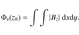
In the emergence process not all the flux is transported into the
atmosphere, some remains in the solar interior and at the base of the
photosphere. To quantify how much flux emerges and how much does not we
consider the horizontal flux, through the central y=0 plane,
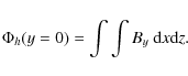
This integral is calculated for the regions above and below the base of the photosphere (z=0). These values are shown in Figs. 13 and 14 as percentages of the initial
![\begin{figure}
\par\includegraphics[width=7.5cm,clip]{12930f13.eps}
\end{figure}](/articles/aa/full_html/2009/44/aa12930-09/img101.png)
|
Figure 13:
The evolution of
|
| Open with DEXTER | |
![\begin{figure}
\par\includegraphics[width=7.5cm,clip]{12930f14.eps}
\end{figure}](/articles/aa/full_html/2009/44/aa12930-09/img102.png)
|
Figure 14:
The evolution of
|
| Open with DEXTER | |
3.3 Plasma drainage
We have answered the first part of question one, which was asked in
the Introduction, by showing that the original axis of a toroidal tube,
with sufficiently strong B0,
can emerge to the corona. However, the problem of why this happens in
the toroidal model and not in the standard cylindrical model remains to
be confronted. Murray et al. (2006) carry out a parameter study for the cylinder model. For a tube of B0=9 they find the maximum height of the original tube axis reaches
![]() .
The main difference between the two models lies in the geometry. The
legs of the toroidal model rise steeply as the whole arch of the tube
rises to emerge. The cylinder model, however, with its exponential
buoyancy profile, kinks in the centre of the tube. The buoyant section
increases as the tube rises higher.
.
The main difference between the two models lies in the geometry. The
legs of the toroidal model rise steeply as the whole arch of the tube
rises to emerge. The cylinder model, however, with its exponential
buoyancy profile, kinks in the centre of the tube. The buoyant section
increases as the tube rises higher.
As the cylinder model emerges, plasma draining from the emerged arcade flows down to the photosphere and collects in multiple dips where the axis is trapped (Archontis et al. 2009). In the toroidal model, flows exist in the legs of the tubes that correspond to draining downflows. Figures 15 and 16 show a cut of uz through one of the legs for the B0=7 case at t=40,50, respectively. At t=40 the tube is buoyantly rising and the vertical velocity in the cut is positive. By t=50, however, plasma begins to drain down the arcade and also down the legs of the tube. There is a change in sign in the velocity of the cut and this corresponds to a draining downflow. The geometry of the toroidal model allows the plasma to drain down the legs and not collect in dips. It is this property that allows the original axis of the tube to emerge.
![\begin{figure}
\par\includegraphics[width=7.5cm,clip]{12930f15.eps}
\end{figure}](/articles/aa/full_html/2009/44/aa12930-09/img104.png)
|
Figure 15: The vertical velocity profile through a cut in one of the legs of the toroidal tube at t=40 and (x,y)=(0,-13). The vertical velocity in the cut is positive since the tube is buoyantly rising. |
| Open with DEXTER | |
![\begin{figure}
\par\includegraphics[width=7.5cm,clip]{12930f16.eps}
\end{figure}](/articles/aa/full_html/2009/44/aa12930-09/img105.png)
|
Figure 16: The vertical velocity profile through a cut in one of the legs of the toroidal tube at t=50 and (x,y)=(0,-13). The sign of the velocity in the cut has now changed since plasma drains down the leg, creating a downflow. |
| Open with DEXTER | |
To determine whether or not the axis can emerge in the cylinder
model, we perform a simple test. Instead of using the the standard
buoyancy profile of
![]() ,
we consider
,
we consider
where n is a positive integer. This is a generalisation of the standard profile (n=1) and will make the central part of the tube buoyant and the ends of the tube over dense. The size of the buoyant region is controlled by n and
![\begin{figure}
\par\includegraphics[height=7cm,width=8cm,clip]{12930f17.eps}
\end{figure}](/articles/aa/full_html/2009/44/aa12930-09/img111.png)
|
Figure 17:
The geometry of the cylinder model with the buoyancy profile
|
| Open with DEXTER | |
As mentioned at the beginning of this section, Murray et al. (2006) found that the axis of a tube with B0=9 and
![]() rises to a maximum height of
rises to a maximum height of
![]() .
In our experiment the, now arched, cylinder axis has risen far beyond this. By t=86 the height of the axis is
.
In our experiment the, now arched, cylinder axis has risen far beyond this. By t=86 the height of the axis is
![]() ,
the base of the transition region. This confirms that it is the
geometry of the toroidal model that enables the efficient draining of
plasma and so allows the axis to emerge.
,
the base of the transition region. This confirms that it is the
geometry of the toroidal model that enables the efficient draining of
plasma and so allows the axis to emerge.
This may help to explain why flux emergence studies that include convection (Tortosa-Andreu & Moreno-Insertis 2009; Cheung et al. 2007) find that the axis of the cylindrical tube emerges. If convective flows can change the geometry of the tube from cylindrical to toroidal, then the axis can emerge as in our experiment.
3.4 Varying  with fixed B0
In this section we investigate the effect of varying the initial twist ![]() .
We will consider the evolution of tubes with
.
We will consider the evolution of tubes with ![]() = 0.2, 0.3, 0.4. We will take B0=7
for all these cases since, as described in the previous section, this
value results in the tube axis emerging with the field around the axis
being vertical at the centre of the sunspots. All tubes have an initial
minor radius r0=2.5 and major radius s0=15.
= 0.2, 0.3, 0.4. We will take B0=7
for all these cases since, as described in the previous section, this
value results in the tube axis emerging with the field around the axis
being vertical at the centre of the sunspots. All tubes have an initial
minor radius r0=2.5 and major radius s0=15.
3.4.1 Rise and emergence
The twist of the magnetic field of a flux tube results in a tension
force acting on the tube. At the top of the initial toroidal tube the
density deficit at the axis is given by
The smaller the value of
![\begin{figure}
\par\includegraphics[width=7.5cm,clip]{12930f18.eps}
\end{figure}](/articles/aa/full_html/2009/44/aa12930-09/img114.png)
|
Figure 18:
The axis height-time profiles for the cases
|
| Open with DEXTER | |
Once the tube reaches the photosphere, it slows down and then emerges by means of a buoyancy instability (Murray et al. 2006).
To investigate how the initial twist influences the emergence, we look
at how the unsigned vertical flux evolves with time. The total unsigned
vertical flux in a plane (z=z0) is defined by
Here we will consider the
![\begin{figure}
\par\includegraphics[width=7.5cm,clip]{12930f19.eps}
\end{figure}](/articles/aa/full_html/2009/44/aa12930-09/img117.png)
|
Figure 19:
The amount of twist affects the amount of flux that emerges into the atmosphere. Key:
|
| Open with DEXTER | |
![\begin{figure}
\par\includegraphics[width=7.5cm,clip]{12930f20.eps}
\end{figure}](/articles/aa/full_html/2009/44/aa12930-09/img118.png)
|
Figure 20:
The amount of twist affects the amount of flux that emerges into the atmosphere. Key:
|
| Open with DEXTER | |
The
![]() case rises to the photosphere before the
case rises to the photosphere before the
![]() case. At the photosphere, however, the smaller twist case takes longer
to become subject to the buoyancy instability than the larger one. This
means that both cases emerge at approximately the same time. Murray et al. (2006)
found similar behaviour for the cylinder model. They studied the
buoyancy instability by considering a local analysis at the
photosphere. Once emerged, the field of the
case. At the photosphere, however, the smaller twist case takes longer
to become subject to the buoyancy instability than the larger one. This
means that both cases emerge at approximately the same time. Murray et al. (2006)
found similar behaviour for the cylinder model. They studied the
buoyancy instability by considering a local analysis at the
photosphere. Once emerged, the field of the
![]() case rises faster and further than the
case rises faster and further than the
![]() case. This is shown in Fig. 19. Figure 20 shows the evolution of
case. This is shown in Fig. 19. Figure 20 shows the evolution of ![]() for
for
![]() begins before that of
begins before that of
![]() .
It also rises at a faster rate and by t=94 there is double the amount of unsigned vertical flux compared with the
.
It also rises at a faster rate and by t=94 there is double the amount of unsigned vertical flux compared with the
![]() case. When at the photosphere, the field for the
case. When at the photosphere, the field for the
![]() case was weaker than that of the
case was weaker than that of the
![]() case. Therefore, the field emerging into the atmosphere is also weaker,
resulting in a weaker evolution of the total unsigned flux.
case. Therefore, the field emerging into the atmosphere is also weaker,
resulting in a weaker evolution of the total unsigned flux.
3.4.2 Sunspot drift
![\begin{figure}
\par\includegraphics[width=7.5cm,clip]{12930f21.eps}
\end{figure}](/articles/aa/full_html/2009/44/aa12930-09/img119.png)
|
Figure 21:
The y-separation in time of the maximum and minimum Bz at the base of the photosphere (z=0). The higher the twist, the slower the separation. Key:
|
| Open with DEXTER | |
A simulation drawback of the cylinder model, which has become the
standard in numerical flux emergence, is that the sunspot pair it
produces continually drifts apart until it reaches the edge of the
computational box. Although a density deficit is introduced into the
tube to form an ![]() -loop, the entire tube is in fact buoyant since the
-loop, the entire tube is in fact buoyant since the
![]() profile makes the ends of the tube weakly buoyant. This is what causes
the sunspots to drift apart. In the toroidal model, although the entire
tube is made buoyant, the ``feet'' of the flux tube are held at a fixed
distance apart in the solar interior. Figure 21 shows the y-separation of the maximum and minimum Bz the base of the photosphere (z=0) for the twist cases
profile makes the ends of the tube weakly buoyant. This is what causes
the sunspots to drift apart. In the toroidal model, although the entire
tube is made buoyant, the ``feet'' of the flux tube are held at a fixed
distance apart in the solar interior. Figure 21 shows the y-separation of the maximum and minimum Bz the base of the photosphere (z=0) for the twist cases
![]() .
As described above, the lower the twist, the faster the rise to the
photosphere. Once the tubes reach the photosphere, the fields begin to
spread. The sunspot separation increases linearly until a peak distance
is reached and the y-separation
remains approximately constant. This peak distance corresponds to the
major diameter of the initial tube. In this example, 2s0=30.
The constancy of the separation between the two main opposite
polarities (sunspots) in an active region is often used as a criterion
for the region's maturity (Liu & Zhang 2006).
Tubes of a higher twist will spread laterally more slowly than tubes of
a lower twist since a higher twist produces a stronger tension force.
The slopes for the linear separation phase are estimated to
be 0.833 for
.
As described above, the lower the twist, the faster the rise to the
photosphere. Once the tubes reach the photosphere, the fields begin to
spread. The sunspot separation increases linearly until a peak distance
is reached and the y-separation
remains approximately constant. This peak distance corresponds to the
major diameter of the initial tube. In this example, 2s0=30.
The constancy of the separation between the two main opposite
polarities (sunspots) in an active region is often used as a criterion
for the region's maturity (Liu & Zhang 2006).
Tubes of a higher twist will spread laterally more slowly than tubes of
a lower twist since a higher twist produces a stronger tension force.
The slopes for the linear separation phase are estimated to
be 0.833 for
![]() ,
0.815 for
,
0.815 for
![]() and 0.8 for
and 0.8 for
![]() .
.
The maximum separation of the sunspots in these simulations is determined by the distance of the almost vertical flux tube legs at the base of the numerical box. This has consequences for the structure of the magnetic field in the interior. The classic picture of flux emergence, as described in the Introduction, considers flux tubes with long wavelengths in the convection zone, typically generated by m=1, 2 instabilities at the tachocline, where m is the longitudinal wavenumber. In the local Cartesian approximation near the surface, this can be represented by the cylinder model. The toroidal model, on the other hand, has vertical legs. There are two possible mechanisms for forming toroidal tubes in the convection zone. Either the modification of the cylindrical tube takes the form of that described in Sect. 3.3, namely the (enhanced) buoyant region of the cylindrical tube is spatially limited and takes effect deeper in the convection zone (rather than near the photosphere as in previous simulations) or the instability, at the base of the convection zone, involves a higher longitudinal mode, e.g. m > 10. Both cases would produce toroidal shaped tubes with almost vertical legs.
4 Conclusions
In this paper we have carried out a parametric study of the emergence of buoyant toroidal
flux tubes through the solar interior and into the atmosphere, via
3D MHD simulations. By varying two of the parameters, namely B0 and ![]() ,
we have been able to investigate the general behaviour of the emerging tubes.
,
we have been able to investigate the general behaviour of the emerging tubes.
Keeping ![]() constant, the variation of the initial field strength produces a wealth
of behaviour. In the solar interior the buoyancy force is proportional
to B02. Tubes with stronger B0
rise faster and further than those with lower values. In the solar
interior the tubes exhibit a self-similar behaviour. By rescaling the
time to
constant, the variation of the initial field strength produces a wealth
of behaviour. In the solar interior the buoyancy force is proportional
to B02. Tubes with stronger B0
rise faster and further than those with lower values. In the solar
interior the tubes exhibit a self-similar behaviour. By rescaling the
time to
![]() ,
the axis height-time profiles for the different B0 lie on top of each other (Murray et al. 2006). This shows that the axis heights of the tubes are not only a function of time but also of B0.
,
the axis height-time profiles for the different B0 lie on top of each other (Murray et al. 2006). This shows that the axis heights of the tubes are not only a function of time but also of B0.
Once emerged, the evolution of the tubes can vary strongly depending on the choice of the initial field strength. A value between B0=5 and B0=7 gives a threshold between two general classes of behaviour. For the B0=7 case, the axis rises fast enough to emerge into the atmosphere before plasma draining from the field above flows into a pressure deficit and blocks its ascent. The plasma instead drains below the axis and produces reconnection upflows that further increase the height of the axis. For the B0=5 case, the axis does not rise fast enough to escape plasma draining on top of it and so is pinned down in the photosphere.
An advantage of the the toroidal model over the standard cylinder model in flux emergence is that the axis of the original tube is able to emerge into the atmosphere and so the field at the centre of the sunspots is vertical. This is made possible by the ability of the the plasma to drain down the legs of the tube in the solar interior. In the cylinder model such draining is not possible and plasma collects in dips along the tube axis. It has been shown, however, that by changing the buoyancy profile to produce a toroidal shape, the tube axis can achieve greater heights in the solar atmosphere.
Keeping B0 constant, the variation in ![]() also
produces interesting behaviour. In the solar interior it is found that
tubes with lower twists rise faster than tubes with higher twists. Once
at the photosphere, however, low twist tubes take longer to become
subject to the magnetic buoyancy instability. This allows higher twist
tubes to catch up and emerge approximately at the same time.
also
produces interesting behaviour. In the solar interior it is found that
tubes with lower twists rise faster than tubes with higher twists. Once
at the photosphere, however, low twist tubes take longer to become
subject to the magnetic buoyancy instability. This allows higher twist
tubes to catch up and emerge approximately at the same time.
It is found that the amount of flux emerged into the atmosphere depends on the value of ![]() .
The higher the twist the more flux is transported upwards. In the rise
of a flux tube, the stronger the twist, the more preserved the tube
remains. The field strength of higher twisted tubes is stronger than
lower twisted tubes when they emerge. This manifests itself in the
amount of flux that is transported into the atmosphere.
.
The higher the twist the more flux is transported upwards. In the rise
of a flux tube, the stronger the twist, the more preserved the tube
remains. The field strength of higher twisted tubes is stronger than
lower twisted tubes when they emerge. This manifests itself in the
amount of flux that is transported into the atmosphere.
Another feature of the toroidal model, which improves upon the cylinder model, is that the sunspots drift to a fixed separation and then stop. This separation is determined by the major diameter of the original tube. The y-separation of the maximum and minimum values of Bz increases linearly until the maximum separation is reached, the diameter of the tube. The higher the twist of the the tube, the slower the separation rate.
This study has revealed many important aspects of the emergence of toroidal tubes and there are many directions for future work to follow, such as the inclusion of convection into the model to study how it affects the emergence and eventual break up of active regions and the interaction of multiple loops to model solar atmospheric events.
AcknowledgementsD.M. acknowledges financial assistance from STFC. Part of the computational work for this paper was carried out on the joint STFC and SFC (SRIF) funded cluster at the University of St Andrews. D.M. and A.W.H. acknowledge financial support from the European Commission through the SOLAIRE Network (MTRN-CT-2006-035484). D.M. and A.W.H. would also like to thank the referee for helpful and constructive comments.
References
- Arber, T. D., Longbottom, A. W., Gerrard, C. L., et al. 2001, J. Comput. Phys., 171, 151 [CrossRef] [NASA ADS]
- Archontis, V. 2008, J. Geophys. Res., 113, Issue A3
- Archontis, V., & Török, T. 2008, A&A, 492, L35 [EDP Sciences] [CrossRef] [NASA ADS]
- Archontis, V., Hood, A. W., Sacheva, A., Golub, L., & Deluca, E. 2009, ApJ, 691, 1291 [CrossRef] [NASA ADS]
- Cheung, M. C. M., Schüssler, M., & Moreno-Insertis, F. 2006, A&A, 467, 703 [CrossRef] [NASA ADS]
- Cowling, T. G. 1946, MNRAS, 106, 218 [NASA ADS]
- Emonet, T., & Moreno-Insertis, F. 1998, ApJ, 492, 804 [CrossRef] [NASA ADS]
- Fan, Y. 2001, ApJ, 554, L111 [CrossRef] [NASA ADS]
- Fan, Y. 2008, ApJ, 676, 680 [CrossRef] [NASA ADS]
- Heinemann, T., Nordlund, Å., Scharmer, G. B., et al. 2007, ApJ, 669, 1390 [CrossRef] [NASA ADS]
- Hood, A. W., Archontis, V., Galsgaard, K. G. et al. 2009, A&A, 503, 999 [EDP Sciences] [CrossRef] [NASA ADS]
- Jensen, E. 1955, Ann. Astrophys., 18, 127 [NASA ADS]
- Jouve, L., & Brun, A. S. 2007, Astron. Nachr., 328, 1104 [CrossRef] [NASA ADS]
- Liu, J., & Zhang, H. 2006, Sol. Phys., 234, 21 [CrossRef] [NASA ADS]
- MacTaggart, D., & Hood, A. W. 2009, A&A, 501, 761 [EDP Sciences] [CrossRef] [NASA ADS]
- Magara, T., & Loncope, D. W. 2003, ApJ, 586, 630 [CrossRef] [NASA ADS]
- Manchester IV, W. 2001, ApJ, 147, 503 [CrossRef] [NASA ADS]
- Manchester IV, W., Gombosi, T., DeZeeuw, D., et al. 2004, ApJ, 610, 588 [CrossRef] [NASA ADS]
- Murray, M. J., Hood, A. W., Moreno-Insertis, F., Galsgaard, K., & Archontis, V. 2006, A&A, 460, 909 [EDP Sciences] [CrossRef] [NASA ADS]
- Parker, E. N. 1955, ApJ, 121, 491 [CrossRef] [NASA ADS]
- Petrie, G. J. D., & Neukirch, T. 1999, Geophys. Astrophys. Fluid Dynam., 91, 269 [CrossRef] [NASA ADS]
- Thomas, J. H., & Weiss, N. O. 1992, Sunspots: Theory and Observations (Kluwer Academic Publishers)
- Thomas, J. H., & Weiss, N. O. 2008, Sunspots and Starspots (Cambridge University Press)
- Tortosa-Andreu, A., & Moreno-Insertis, F. 2009, A&A, 507, 949 [EDP Sciences] [CrossRef]
All Figures
|
|
Figure 1: The height-time profiles for axes with different B0 traced in the y=0 plane. Key: B0=1 (solid), B0=3 (dot), B0=5 (dash), B0=7 (dot-dash) and B0=9 (triple dot-dash). |
| Open with DEXTER | |
| In the text | |
|
|
Figure 2:
The height-time profiles in the solar interior rescaled to time
|
| Open with DEXTER | |
| In the text | |
|
|
Figure 3: This diagram illustrates some of the main dynamical features of the emergence of a toroidal flux tube. The outline represents the outermost field line of the emerging arcade. See the text for more details. |
| Open with DEXTER | |
| In the text | |
|
|
Figure 4: The density deficit at the tube axis (in the y=0 plane) as a fraction of the initial unsigned density deficit against height. Key: B0=5 (dash), B0=7 (solid). |
| Open with DEXTER | |
| In the text | |
|
|
Figure 5:
The vertical velocity, uz, (in the y=0 plane) as a function of height.
|
| Open with DEXTER | |
| In the text | |
|
|
Figure 6: The ``square well'' profile for the deficit in the total pressure. This deficit exists for a finite range of heights (see text) and plasma draining from above flows into it. This figure is for the B0=7 case at t=100 and (y,z)=(0,3). |
| Open with DEXTER | |
| In the text | |
|
|
Figure 7: The B0=5 case at t=100. The original tube axis is represented by a red field line. Some surrounding field lines are traced in grey. A magnetogram is placed at the bottom of the photosphere (z=0) and shows Bz. |
| Open with DEXTER | |
| In the text | |
|
|
Figure 8: The B0=7 case at t=100. The original tube axis is represented by a red field line. Some surrounding field lines are traced in grey. A magnetogram is placed at the bottom of the photosphere (z=0) and shows Bz. |
| Open with DEXTER | |
| In the text | |
|
|
Figure 9: Shearing profiles at t=100 and (y,z)=(0,3) for B0=5 (dash) and B0=7 (solid). |
| Open with DEXTER | |
| In the text | |
|
|
Figure 10: Inflow profiles at t=100 and (y,z)=(0,3) for B0=5 (dash) and B0=7 (solid). There are clear inflow profiles for both cases. However, when the flows meet in the centre of the pressure deficit zone, they produce more complex behaviour. |
| Open with DEXTER | |
| In the text | |
|
|
Figure 11: The B0=5 case at t=100. The red field line represents the original tube axis. The green field line represents the axis of a new flux rope. The surrounding field line structure at the new axis is demonstrated by some field lines traced in grey. The original axis is pinned down in the photosphere whereas the new rope is at the base of the corona. The magnetogram is at z=0. |
| Open with DEXTER | |
| In the text | |
|
|
Figure 12: The B0=7 case at t=100. The red field line represents the original tube axis. The green field line represents the axis of a new flux rope. The surrounding field line structure at the new axis is demonstrated by some field lines traced in grey. Reconnection occurs where the grey field lines cross. An upward jet from this pushes the original axis higher. The magnetogram is at z=0. |
| Open with DEXTER | |
| In the text | |
|
|
Figure 13:
The evolution of
|
| Open with DEXTER | |
| In the text | |
|
|
Figure 14:
The evolution of
|
| Open with DEXTER | |
| In the text | |
|
|
Figure 15: The vertical velocity profile through a cut in one of the legs of the toroidal tube at t=40 and (x,y)=(0,-13). The vertical velocity in the cut is positive since the tube is buoyantly rising. |
| Open with DEXTER | |
| In the text | |
|
|
Figure 16: The vertical velocity profile through a cut in one of the legs of the toroidal tube at t=50 and (x,y)=(0,-13). The sign of the velocity in the cut has now changed since plasma drains down the leg, creating a downflow. |
| Open with DEXTER | |
| In the text | |
|
|
Figure 17:
The geometry of the cylinder model with the buoyancy profile
|
| Open with DEXTER | |
| In the text | |
|
|
Figure 18:
The axis height-time profiles for the cases
|
| Open with DEXTER | |
| In the text | |
|
|
Figure 19:
The amount of twist affects the amount of flux that emerges into the atmosphere. Key:
|
| Open with DEXTER | |
| In the text | |
|
|
Figure 20:
The amount of twist affects the amount of flux that emerges into the atmosphere. Key:
|
| Open with DEXTER | |
| In the text | |
|
|
Figure 21:
The y-separation in time of the maximum and minimum Bz at the base of the photosphere (z=0). The higher the twist, the slower the separation. Key:
|
| Open with DEXTER | |
| In the text | |
Copyright ESO 2009
Current usage metrics show cumulative count of Article Views (full-text article views including HTML views, PDF and ePub downloads, according to the available data) and Abstracts Views on Vision4Press platform.
Data correspond to usage on the plateform after 2015. The current usage metrics is available 48-96 hours after online publication and is updated daily on week days.
Initial download of the metrics may take a while.