| Issue |
A&A
Volume 507, Number 2, November IV 2009
|
|
|---|---|---|
| Page(s) | 855 - 860 | |
| Section | Interstellar and circumstellar matter | |
| DOI | https://doi.org/10.1051/0004-6361/200912825 | |
| Published online | 15 September 2009 | |
A&A 507, 855-860 (2009)
The interaction of an O star wind with a Herbig-Haro jet
A. Esquivel1 - A. C. Raga1 - J. Cantó2 - A. Rodríguez-González1
1 - Instituto de Ciencias Nucleares, Universidad Nacional
Autónoma de México, Ap. Postal 70-543, 04510 D.F., México
2 - Instituto de Astronomía, Universidad Nacional
Autónoma de México, Ap. Postal 70-468, 04510 D.F., México
Received 3 July 2009 / Accepted 4 September 2009
Abstract
Context. Herbig-Haro jets ejected from young, low mass stars
in the proximity of O/B stars will interact with the more or less
isotropic winds from the more massive stars. An example of this are the
jets from the stars within the proplyds near ![]() -Orionis.
-Orionis.
Aims. In this paper, we consider the interaction of an
externally photoionized HH jet with an isotropic wind ejected from the
ionizing photon source. We study this problem through numerical
simulations, allowing us to obtain predictions of the detailed
structure of the flow and predictions of H![]() intensity maps. This is a natural extension of a previously developed
analytic model for the interaction between a jet and an isotropic
stellar wind.
intensity maps. This is a natural extension of a previously developed
analytic model for the interaction between a jet and an isotropic
stellar wind.
Methods. We present 3D simulations of a bipolar HH jet
interacting with an isotropic wind from a massive star, assuming that
the radiation from the star photoionizes all of the flow. We describe
different possible flow configurations, exploring a limited set of jet
and stellar wind parameters and orientations of the jet/counterjet
ejection. We have computed 6 models, two of which also include a
time-variability in the jet velocity.
Results. We compare the locus of the computed jet/counterjet
systems with the analytic model, and find very good agreement except
for cases in which the direction of the jet (or the counterjet)
approaches the direction to the wind source (i.e., the O star). For the
models with variable ejection velocities, we find that the internal
working surfaces follow straighter trajectories (and the inter-working
surface segments more curved trajectories) than the equivalent steady
jet model.
Key words: ISM: kinematics and dynamics - ISM: jets and outflows - ISM: Herbig-Haro objects - stars: winds, outflows
1 Introduction
In a recent paper, Raga et al. (2009a) presented an analytic model for the interaction of a steady Herbig-Haro (HH) jet (from a young, low mass star) with an isotropic wind (from a more massive, nearby young star). The isotropic wind source could be a Herbig Ae/Be star, or an O/B star.
This model was an extension of the jet/sidewind analytic model of Cantó & Raga (1995), incorporating the divergence of the wind which impinges on the HH jet. The HH jet/plane-parallel sidewind scenario has also been studied with 3D gas-dynamic simulations (Lim & Raga 1998; Masciadri & Raga 2001; Kajdic & Raga 2007; Ciardi et al. 2008), and successful comparisons with the analytic model of Cantó & Raga (1995) have been made.
In this paper, we present 3D gas-dynamic simulations of the interaction between an isotropic wind from an O star and a HH jet. We present models of jets with a steady ejection velocity, and also with a sinusoidally varying velocity. We explore the effects of different parameter combinations, including the direction of ejection (with respect to the direction to the wind source) of the jet/counterjet systems. Comparisons with the analytic model of Raga et al. (2009a) are carried out.
Our simulations allow us to make predictions of observable
parameters. In particular, we present H![]() emission line maps,
which in principle can be compared with images of candidate systems.
emission line maps,
which in principle can be compared with images of candidate systems.
It is actually not clear to which objects our O star wind/HH jet
model could be applied. Possible candidates are the jets ejected
from the proplyds located within or in the proximity of
the ![]() -Ori Trapezium in M42, such as HH 508, HH 514
and the jet/counterjet system that is possibly being powered
by the 167-317 (LV2) proplyd (see Bally et al. 2000).
These systems are likely to be embedded within the stellar winds of
the
-Ori Trapezium in M42, such as HH 508, HH 514
and the jet/counterjet system that is possibly being powered
by the 167-317 (LV2) proplyd (see Bally et al. 2000).
These systems are likely to be embedded within the stellar winds of
the ![]() -Ori stars, and therefore represent possible jet/wind
interaction systems.
Unfortunately, these jets are barely detected in HST images, with
identified lengths of
-Ori stars, and therefore represent possible jet/wind
interaction systems.
Unfortunately, these jets are barely detected in HST images, with
identified lengths of ![]() 1''. Therefore, it is not possible
to say whether or not they curve away from the stellar wind sources,
as expected.
1''. Therefore, it is not possible
to say whether or not they curve away from the stellar wind sources,
as expected.
The much larger scale, curved jets seen at larger distances from
![]() -Ori (see Bally & Reipurth 2001; Bally et al. 2006)
are not immersed in the wind from the
-Ori (see Bally & Reipurth 2001; Bally et al. 2006)
are not immersed in the wind from the ![]() -Ori stars, and
are interacting with the expanding M42 nebula. Therefore, they
are not candidates for modeling with the simulations described
in the present paper.
-Ori stars, and
are interacting with the expanding M42 nebula. Therefore, they
are not candidates for modeling with the simulations described
in the present paper.
This lack of a clear astrophysical counterpart for the simulations of the present paper is of course somewhat problematic. At the end of the paper, we discuss what kind of observations are necessary in order to solve this problem.
The paper is organized as follows. The analytic model of Raga et al. (2009a) is summarized in Sect. 2. The setup of the numerical simulations is described in Sect. 3. A description of the results and comparisons with the analytic model of Raga et al. (2009a) are presented in Sect. 4. Predictions of observable quantities are discussed in Sects. 5 and 6. Finally, the results are summarized in Sect. 7.
2 The analytic model
The shape of a jet/counterjet system, immersed in an external wind, can be obtained balancing the ram pressure of the wind (impinging on the side of the jet) with the centrifugal pressure of the material along the curved jet path. Cantó & Raga (1995) modeled the interaction of a plane-parallel wind with a jet, assuming that the cross section of the jet is that of an isothermal ``plasmon''. Following the same idea, but adopting a more appropriate coordinate system for the model, the interaction of a jet/counterjet system with an isotropic wind was presented in Raga et al. (2009a).
A schematic of the geometry of the problem is shown in Fig. 1.
![\begin{figure}
\par\includegraphics[width=8cm]{12825f1}
\end{figure}](/articles/aa/full_html/2009/44/aa12825-09/img14.png)
|
Figure 1:
(Reproduced with permission from Raga et al. 2009a)
Schematic of the coordinate system(s) of the analytic model of
the interaction of a HH jet and a star. Top frame:
the star is placed at the origin of the xy-coordinate
system, and the ``stagnation point'' (point of maximum approach
between the star and the jet/counterjet path) is aligned with the
x-axis. The jet/counterjet locus is described by |
| Open with DEXTER | |
Table 1:
Model parameters
![]()
Balancing the ram pressure that the stellar wind exerts on the side of
the jet, with the centrifugal force of the jet following a curved
trajectory such that its cross section preserves an
isothermal plasmon shape, we obtain the differential
equation
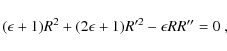
where the dimensionless parameter
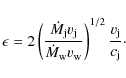
This equation can be integrated two times (with the appropriate boundary conditions) to obtain
where

thus, the total deflection angle is
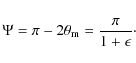
The solution is symmetrical with respect to the x-axis (the line that passes through the star and the stagnation point), and for a given stagnation distance
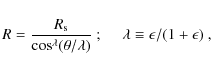
Alternatively, one could write the solution in the primed reference
system (the abscissa aligned with the wind and jet sources, see
Fig. 1). To do this one has to note that
and use the solution in Eq. (3) to find a relation between the angles

This can be used to obtain
![\begin{displaymath}R_{{\rm s}}=D\left[\sin\alpha\right]^\lambda~.
\end{displaymath}](/articles/aa/full_html/2009/44/aa12825-09/img46.png)
Finally, combining Eqs. (7)-(8) with
![\begin{displaymath}R(\theta')=D\left[{\sin\alpha\over {\sin\left(\alpha-\theta'/\lambda\right)}}
\right]^\lambda\cdot
\end{displaymath}](/articles/aa/full_html/2009/44/aa12825-09/img48.png)
This expression is useful to constrain
3 The numerical simulations
3.1 The code
We used a 3D hydrodynamical code to compute 6 different models of the interaction of a massive star with a HH jet. The code integrates the gas-dynamic equations on a regular, uniform Cartesian grid, using a second order finite volume method with HLLC fluxes (Toro et al. 1994), and piecewise linear reconstruction with a minmod slope limiter. The code is parallel, with a domain split in blocks arranged in a Cartesian grid, implemented by the Message Passing Interface (MPI) library.
In our simulations H is fully ionized throughout the flow, as a result of the photoionizing radiation from the O star. We do not consider the possibility of an ionization front being trapped within the body of the jet (see Masciadri & Raga 2001). In the energy equation, we include a parametrized cooling function (see Raga et al. 2009b for a detailed description). As we have assumed that the flow is fully photoionized, we have imposed a minimum temperature of 104 K, corresponding to the approximate temperature resulting from photoionization equilibrium.
3.2 Numerical setup
We computed 6 models of the interaction of a HH jet with an isotropic
wind, in a cubic computational domain with
![]() per side, and 2563 cells, yielding a resolution of
per side, and 2563 cells, yielding a resolution of
![]() along the three axes.
along the three axes.
A summary of the parameters we used is given in Table 1.
The position of the stellar wind source is fixed in all models,
centered on the yz-plane, located at
![]() from the left boundary along the x-direction.
from the left boundary along the x-direction.
In a sphere of radius
![]() centered at this
position, we inject an isotropic wind with a temperature of
centered at this
position, we inject an isotropic wind with a temperature of
![]() and a terminal velocity
and a terminal velocity
![]() .
Inside the sphere
the density follows an
.
Inside the sphere
the density follows an
![]() law (r being the spherical
radius) scaled so that the mass loss rate is
law (r being the spherical
radius) scaled so that the mass loss rate is
![]() .
.
At a position
![]() from the
wind source, (see Table 1) we place a bipolar cylindrical
jet (with
from the
wind source, (see Table 1) we place a bipolar cylindrical
jet (with
![]() of radius and length),
with a top hat profile and a
of radius and length),
with a top hat profile and a
![]() mass loss rate (for each outflow lobe). The jet/counterjet axis is oriented at an angle
mass loss rate (for each outflow lobe). The jet/counterjet axis is oriented at an angle
![]() with respect to the y-axis, and is always perpendicular to the z-axis. The jet material is injected with a temperature
with respect to the y-axis, and is always perpendicular to the z-axis. The jet material is injected with a temperature
![]() ,
and both the jet and the wind are fully ionized.
,
and both the jet and the wind are fully ionized.
In models M1-M3 the jet source is placed at the stagnation point,
thus the ejection velocity is perpendicular to the wind at that
position. Models M4-M6 are placed along the analytical solution
of the path from models M1-M3, respectively, at the appropriate
off-axis angle. For models M1, M2, M4, and M5 the jet/counterjet
speed is time-independent (
![]() ).
Models M3 and M6 have the same parameters as
M2 and M5, respectively, but have a time-dependent ejection
velocity of the form:
).
Models M3 and M6 have the same parameters as
M2 and M5, respectively, but have a time-dependent ejection
velocity of the form:
4 Results
We let all models evolve until the jet leaves the computational
domain, which varies for each model, but is always of ![]()
![]() .
.
As mentioned above, the analytical model considers the motion in the
plane defined by the jet/counterjet axis and the wind source, which we
have chosen to lie on the xy-plane of our simulations.
In Fig. 2 we present a transverse cut (corresponding to
the
![]() plane) of the
density stratification of model M1, after an integration time of
plane) of the
density stratification of model M1, after an integration time of
![]() .
From this figure, the
plasmon-shaped cross section of the jet is evident.
In the figure we
marked the position of the jet source, we can see that the densest
region (body of the jet) has displaced to the right at this
distance. In addition, we have traced the material ejected by the
wind and jet sources, with a passive scalar that is proportional to the
density but that has opposite sign. The solid line shows the position
where the passive scalar changes sign, to the left we have stellar
wind material, and jet material to the right.
.
From this figure, the
plasmon-shaped cross section of the jet is evident.
In the figure we
marked the position of the jet source, we can see that the densest
region (body of the jet) has displaced to the right at this
distance. In addition, we have traced the material ejected by the
wind and jet sources, with a passive scalar that is proportional to the
density but that has opposite sign. The solid line shows the position
where the passive scalar changes sign, to the left we have stellar
wind material, and jet material to the right.
![\begin{figure}
\par\includegraphics[width=8.8cm]{12825f2}
\end{figure}](/articles/aa/full_html/2009/44/aa12825-09/img65.png)
|
Figure 2:
Cross section of the jet: density stratification in the
|
| Open with DEXTER | |
In Fig. 3 we present cuts of the density stratification on the xy-midplane for all the models after the jet and counterjet have left the grid boundaries. The integration times for each model are indicated in the upper-left hand corner of the panels. Also, for each model, we overlaid the analytical solution of the jet/counterjet locus (dashed curve), and the maximum deflection angle expected, indicated by the arrows in each panel.
![\begin{figure}
\par\includegraphics[width=17cm]{12825f3}
\end{figure}](/articles/aa/full_html/2009/44/aa12825-09/img66.png)
|
Figure 3: The path followed by the jet: density cuts in the xy-midplane in logarithmic scale, as given by the gray-scale bar (colorbar in the online version) at the top, for all models. The model and integration time are indicated in the label at the upper-left corner of each frame. The dashed-line shows the analytical solution of Raga et al. (2009a), and the arrows the expected maximum deflection, obtained from the analytical model as well. |
| Open with DEXTER | |
We can see from Fig. 3 that the paths described by
the jet/counterjet systems in models M1, M2 and M4 agree remarkably
well with the predictions from the analytic model
(see Sect. 2 and Raga et al. 2009a).
These three
models have a constant ejection velocity. In M1 and M2 the jet source
is placed at the stagnation point (therefore the jet is ejected
perpendicularly to the stellar wind). Model M4 has the same parameters
as M1, but is placed off the axis formed by the stagnation point and
the star, however due to the small ![]() parameter it also makes
a large angle with the direction of the wind.
parameter it also makes
a large angle with the direction of the wind.
The jet source of model M5, which is otherwise identical to M2, is almost aligned against the wind source. The resulting jet becomes unstable and breaks before reaching the theoretical stagnation point.
For the models with a variable ejection velocity we obtain very similar results. Model M3, (that corresponds to model M2 plus a sinusoidal velocity variation) shows a series of internal working surfaces that open up as they travel away from the jet source. The internal working surfaces are denser, and follow straighter trajectories than the analytical model. At the same time the regions between the successive working surfaces have trajectories that curve more than the analytical model. Model M6, which also has a time-variable ejection velocity, but is closely directed with the direction towards the star (like M5), shows the same trends observed in the other models. As with model M3, the internal working surfaces follow straighter paths than the constant injection counterpart (M5), while the inter-knot regions are swept more easily by the stellar wind, and therefore are more curved. However, as observed as well in model M5, the jet is considerably slowed by the stellar wind, and reaches its maximum approach before reaching the x-axis, which is where the stagnation point should be according to the analytical model.
The departures from the analytical predictions seen in models M5 and M6 are not surprising. The model considers that the jet adopts the plasmon configuration derived from the plane parallel model (Cantó & Raga 1995). Therefore, the model is only valid when the scale-length of the jet cross section is small compared with the radius of curvature of the path.
5 H emission
![\begin{figure}
\par\includegraphics[width=17cm]{12825f4}
\vspace*{-3.5mm}
\end{figure}](/articles/aa/full_html/2009/44/aa12825-09/img68.png)
|
Figure 4:
H maps for all the models. The
maps have been computed assuming that the observer is located in
the -z-direction. The H intensity in
|
| Open with DEXTER | |
In this section, we present H![]() emission maps computed assuming
that the xy-plane of the simulations (which includes the O star and
the outflow axis) is parallel to the plane of the sky. The results
obtained from models M1-M6 (for the same time-frames as
Fig. 3) are shown in Fig. 4.
emission maps computed assuming
that the xy-plane of the simulations (which includes the O star and
the outflow axis) is parallel to the plane of the sky. The results
obtained from models M1-M6 (for the same time-frames as
Fig. 3) are shown in Fig. 4.
The time-independent ejection velocity models (models M1, M2, M4 and M5, see 1 and Fig. 4) show a more or less continuous emission from the body of the curved jet beam. This emission is a result of the fact that the jet beam is fully photoionized.
The time-dependent ejection velocity models (models M3 and M6,
see Fig. 4), show strong H![]() emission from the
internal working surfaces, and only very weak emission from the
jet beam segments in between the working surfaces. The emission
from the individual working surfaces shows a ``tadpole''-like
morphology, with the ``head'' towards the O star, and the
``tail'' cutting across the curved jet axis.
emission from the
internal working surfaces, and only very weak emission from the
jet beam segments in between the working surfaces. The emission
from the individual working surfaces shows a ``tadpole''-like
morphology, with the ``head'' towards the O star, and the
``tail'' cutting across the curved jet axis.
This remarkable morphology has not yet been observed in any HH object.
Therefore, this represents a prediction of what is expected to
be observed when chains of knots along jets embedded in an O star
wind (e. g., the jets from the proplyds close to ![]() Ori)
are detected.
Ori)
are detected.
6 X-ray emission
It is interesting to note that even though the models described
above do not produce an appreciable amount of X-ray emission,
for appropriate parameters an O-star wind/jet interaction can indeed
produce a substantial X-ray luminosity
![]() .
In order to demonstrate
this, we derive a simple analytic model for computing
.
In order to demonstrate
this, we derive a simple analytic model for computing
![]() .
.
We do this following the ideas of Raga et al. (2002), who derived
an analytic model that predicts the X-ray luminosity from the head
of a HH jet. Following these authors, we note that the X-ray luminosity
is dominated by free-free emission, which has an emission rate
(integrated over all frequencies):
where the temperature T and the number density n (of H ions or of free electrons) are in cgs units (see e.g., Osterbrock 1989).
We now assume that the X-ray emission from the bow shock formed by the
O star wind impinging on the jet beam is dominated by the head
of the bow shock. From the strong shock jump conditions, one
finds that the gas in this region has a temperature
and a number density
where
Finally, we estimate the emitting volume (for a length dl along
the jet) as:
where
We can then compute the X-ray luminosity as
This integral can be computed analytically if one assumes that the X-ray emission is spatially limited to a region close to the stagnation point (see Fig. 1), so that we can neglect the curvature of the jet trajectory, and that
where
However, for stagnation distances
![]() cm (one order of magnitude lower than the
ones of our simulations, see Sect. 3.2) Eq. (16) gives
cm (one order of magnitude lower than the
ones of our simulations, see Sect. 3.2) Eq. (16) gives
![]() .
This luminosity is similar
to the (reddening-corrected)
.
This luminosity is similar
to the (reddening-corrected)
![]() X-ray luminosity estimated from
the Chandra observations of HH 2 Pravdo et al. (2001), so that
the emission could clearly be detected for such an object at the
distance of the Orion nebula.
X-ray luminosity estimated from
the Chandra observations of HH 2 Pravdo et al. (2001), so that
the emission could clearly be detected for such an object at the
distance of the Orion nebula.
7 Summary
We presented 3D numerical simulations of a bipolar HH jet interacting with an isotropic stellar wind from an O star. The results from our simulations can be summarized as follows :
- The jet/isotropic wind interaction leads to the formation of a plasmon-shaped jet cross section (see Fig. 2) and a curved trajectory (see Fig. 3) for the jet beam.
- Constant ejection velocity jet/counterjet systems closely follow the curved path predicted by the analytic model of Raga et al. (2009a) (see models M1, M2 and M4 in Fig. 3), except in cases in which the ejection direction lies close to the direction towards the O star (models M5 and M6 in Fig. 3).
- Jets with variable ejection velocity have internal working surfaces with straighter trajectories and inter-knot regions with more curved trajectories than equivalent steady jet models (M3 and M6 in Fig. 3).
- We have computed H
 emission maps which can be compared
with observations of HH jets in the vicinity of O stars
Fig. 4.
emission maps which can be compared
with observations of HH jets in the vicinity of O stars
Fig. 4.
- The models predict a peculiar morphology of the individual working surfaces that are formed by a velocity variability, which remains to be observed in HH objects near massive stars.
- We have estimated the X-ray luminosity from a simple
analytic model, the wind/jet interaction in our simulations would
not produce a detectable X-ray luminosity. However, if the
stagnation distance (i.e. point of closest approach between the
jet/counterjet path and the O star) is on the order of

 )
such objects would produce X-ray luminosities as
high as
)
such objects would produce X-ray luminosities as
high as
 .
.
We should point out that the H![]() emission obtained in our models
is rather weak compared to the emission from the H II region
near massive stars (near
emission obtained in our models
is rather weak compared to the emission from the H II region
near massive stars (near ![]() -Ori for instance), thus direct imaging
of these jets is unlikely to reveal their extended morphologies.
However, observations in nearby star formation regions might be possible if the jets can be separated from the H II region in velocity, using for instance Fabry-Pérot interferometry.
-Ori for instance), thus direct imaging
of these jets is unlikely to reveal their extended morphologies.
However, observations in nearby star formation regions might be possible if the jets can be separated from the H II region in velocity, using for instance Fabry-Pérot interferometry.
Interestingly, a number of the Orion proplyds have been
detected in X-rays. Kastner et al. (2005) report (deredened)
X-ray luminosities in the
![]() range for
range for
![]() 100 proplyds. For example, the LV2 (167-317) proplyd
(one of the proplyds which are probably embedded in the
wind from
100 proplyds. For example, the LV2 (167-317) proplyd
(one of the proplyds which are probably embedded in the
wind from ![]() -Ori, see Sect. 1) has an X-ray luminosity
of
-Ori, see Sect. 1) has an X-ray luminosity
of ![]()
![]() .
A fraction of this X-ray luminosity might be the result of the
interaction between the jets associated with this object and the wind
from
.
A fraction of this X-ray luminosity might be the result of the
interaction between the jets associated with this object and the wind
from ![]() Ori C.
Ori C.
This work was supported by the DGAPA (UNAM) grant IN108207, the CONACyT grants 46828-F and 61547, and by the ``Macroproyecto de Tecnologías para la Universidad de la Información y la Computación'' (Secretaría de Desarrollo Institucional de la UNAM). We thank Enrique Palacios, Martín Cruz and Antonio Ramírez for their support of the servers in which the simulations were carried out.
References
- Bally, J., & Reipurth, B. 2001, ApJ, 546, 299 [CrossRef] [NASA ADS]
- Bally, J., O'Dell, C. R., & McCaughrean, M. J. 2000, AJ, 119, 2919 [CrossRef] [NASA ADS]
- Bally, J., Licht, D., Smith, N., et al. 2006, AJ, 131, 473 [CrossRef] [NASA ADS]
- Cantó, J., & Raga, A. C. 1995, MNRAS, 277, 1120 [NASA ADS]
- Ciardi, A., Ampleford, D. J., Lebedev, S. V., et al. 2008, ApJ, 678, 968 [CrossRef] [NASA ADS]
- Kajdic, P., & Raga, A. C. 2007, ApJ, 670, 1173 [CrossRef] [NASA ADS]
- Kastner, J. H., Franz, G., Grosso, N., et al. 2005, ApJS, 160, 511 [CrossRef] [NASA ADS]
- Lim, A. J., & Raga, A. C. 1998, MNRAS, 298, 871 [CrossRef] [NASA ADS]
- Masciadri, E., & Raga, A. C. 2001, AJ, 121, 408 [CrossRef] [NASA ADS]
- Osterbrock, D. E. 1989, Astrophysics of gaseous nebulae and active galactic nuclei (Mill Valley: University Science Books)
- Pravdo, S. H., Feigelson, E. D., Garmire, G., et al. 2001, Nature, 413, 708 [CrossRef] [NASA ADS]
- Raga, A. C., Noriega-Crespo, A., & Velázquez, P. F. 2002, ApJ, 576, L149 [CrossRef] [NASA ADS]
- Raga, A. C., Cantó, J., Rodríguez-González, A., & Esquivel, A. 2009a, A&A, 493, 115 [EDP Sciences] [CrossRef] [NASA ADS]
- Raga, A. C., Henney, W., Vasconcelos, J., et al. 2009b, MNRAS, 392, 964 [CrossRef] [NASA ADS]
- Toro, E. F., Spruce, M., & Speares, W. 1994, Shock Waves, 4, 25 [CrossRef] [NASA ADS]
All Tables
Table 1:
Model parameters
![]()
All Figures
|
|
Figure 1:
(Reproduced with permission from Raga et al. 2009a)
Schematic of the coordinate system(s) of the analytic model of
the interaction of a HH jet and a star. Top frame:
the star is placed at the origin of the xy-coordinate
system, and the ``stagnation point'' (point of maximum approach
between the star and the jet/counterjet path) is aligned with the
x-axis. The jet/counterjet locus is described by |
| Open with DEXTER | |
| In the text | |
|
|
Figure 2:
Cross section of the jet: density stratification in the
|
| Open with DEXTER | |
| In the text | |
|
|
Figure 3: The path followed by the jet: density cuts in the xy-midplane in logarithmic scale, as given by the gray-scale bar (colorbar in the online version) at the top, for all models. The model and integration time are indicated in the label at the upper-left corner of each frame. The dashed-line shows the analytical solution of Raga et al. (2009a), and the arrows the expected maximum deflection, obtained from the analytical model as well. |
| Open with DEXTER | |
| In the text | |
|
|
Figure 4:
H maps for all the models. The
maps have been computed assuming that the observer is located in
the -z-direction. The H intensity in
|
| Open with DEXTER | |
| In the text | |
Copyright ESO 2009
Current usage metrics show cumulative count of Article Views (full-text article views including HTML views, PDF and ePub downloads, according to the available data) and Abstracts Views on Vision4Press platform.
Data correspond to usage on the plateform after 2015. The current usage metrics is available 48-96 hours after online publication and is updated daily on week days.
Initial download of the metrics may take a while.