| Issue |
A&A
Volume 507, Number 2, November IV 2009
|
|
|---|---|---|
| Page(s) | 969 - 980 | |
| Section | The Sun | |
| DOI | https://doi.org/10.1051/0004-6361/200912645 | |
| Published online | 15 September 2009 | |
A&A 507, 969-980 (2009)
Magnetic cloud models with bent and oblate cross-section boundaries
P. Démoulin1 - S. Dasso2,3
1 - Observatoire de Paris, LESIA, UMR 8109 (CNRS), 92195 Meudon
Principal Cedex, France
2 - Instituto de Astronomía y Física del Espacio, CONICET-UBA,
CC. 67, Suc. 28, 1428 Buenos Aires, Argentina
3 - Departamento de Física, Facultad de Ciencias Exactas y
Naturales, Universidad de Buenos Aires, 1428 Buenos Aires, Argentina
Received 5 June 2009 / Accepted 13 August 2009
Abstract
Context. Magnetic clouds (MCs) are formed by
magnetic flux ropes that are ejected from the Sun as coronal mass
ejections. These structures generally have low plasma beta and travel
through the interplanetary medium interacting with the surrounding
solar wind. Thus, the dynamical evolution of the internal magnetic
structure of a MC is a consequence of both the conditions of
its environment and of its own dynamical laws, which are mainly
dominated by magnetic forces.
Aims. With in-situ observations
the magnetic field is only measured along the trajectory of the
spacecraft across the MC. Therefore, a magnetic model is needed to
reconstruct the magnetic configuration of the encountered MC. The main
aim of the present work is to extend the widely used cylindrical model
to arbitrary cross-section shapes.
Methods. The flux rope boundary is parametrized to
account for a broad range of shapes. Then, the internal structure of
the flux rope is computed by expressing the magnetic field as a series
of modes of a linear force-free field.
Results. We analyze the magnetic field profile along
straight cuts through the flux rope, in order to simulate the
spacecraft crossing through a MC. We find that the magnetic
field orientation is only weakly affected by the shape of the MC
boundary. Therefore, the MC axis can approximately be found by
the typical methods previously used (e.g., minimum variance). The
boundary shape affects the magnetic field strength most. The
measurement of how much the field strength peaks along the crossing
provides an estimation of the aspect ratio of the flux-rope
cross-section. The asymmetry of the field strength between the front
and the back of the MC, after correcting for the time evolution (i.e.,
its aging during the observation of the MC), provides an estimation of
the cross-section global bending. A flat or/and bent cross-section
requires a large anisotropy of the total pressure imposed at the MC
boundary by the surrounding medium.
Conclusions. The new theoretical model developed
here relaxes the cylindrical symmetry hypothesis. It is designed to
estimate the cross-section shape of the flux rope using the in-situ
data of one spacecraft. This allows a more accurate determination of
the global quantities, such as magnetic fluxes and helicity. These
quantities are especially important for both linking an observed MC to
its solar source and for understanding the corresponding evolution.
Key words: Sun: coronal mass ejections (CMEs) - Sun: magnetic fields - interplanetary medium
1 Introduction
Magnetic clouds (MCs) are magnetized plasma structures ejected from the Sun as coronal mass ejections. They are characterized by a strongly enhanced magnetic field strength with respect to typical solar wind (SW) values, a smooth and large coherent rotation of the magnetic field vector, and a low proton temperature (e.g., Burlaga et al. 1981; Klein & Burlaga 1982). Moreover, after decades of researches, there is presently a consensus that MCs are formed by twisted magnetic flux tubes, called flux ropes (e.g., Burlaga 1995).
The in situ measurements are limited to the spacecraft trajectory crossing the arriving MC. Therefore, one needs to rely on modeling to derive the global magnetic structure from the local measurements. The determination of the proper magnetic configuration for MCs is important in order to provide good estimations of the global magneto-hydrodynamic (MHD) invariants contained in these structures, such as magnetic helicity or fluxes (see, e.g., Démoulin 2008, and references therein).
A key property of MCs is the small plasma ![]() ,
while the plasma velocity in the frame moving with the MC is typically
well below the Alfvén velocity, therefore the magnetic configuration of
MCs is force-free to a first approximation. The magnetic field in MCs
can be relatively well modeled by a linear force-free field (Burlaga 1988). The simplest
solution is obtained with a cylindrical boundary; this is the so-called
Lundquist model (Lundquist 1950).
It was, and is still, widely used to fit the magnetic field observed in
MCs and to derive global quantities such as the magnetic flux and
helicity (e.g., Burlaga 1988;
Lepping et al. 1990;
Dasso et al. 2003; Lynch et al. 2003; Dasso et al. 2005b; Mandrini et al. 2005; Dasso et al. 2006; Leitner et al. 2007).
An extension of this model to an elliptical boundary was realized by Vandas & Romashets (2003).
They derived analytical solutions for any value of the aspect ratio
(ratio of the ellipse sizes).
,
while the plasma velocity in the frame moving with the MC is typically
well below the Alfvén velocity, therefore the magnetic configuration of
MCs is force-free to a first approximation. The magnetic field in MCs
can be relatively well modeled by a linear force-free field (Burlaga 1988). The simplest
solution is obtained with a cylindrical boundary; this is the so-called
Lundquist model (Lundquist 1950).
It was, and is still, widely used to fit the magnetic field observed in
MCs and to derive global quantities such as the magnetic flux and
helicity (e.g., Burlaga 1988;
Lepping et al. 1990;
Dasso et al. 2003; Lynch et al. 2003; Dasso et al. 2005b; Mandrini et al. 2005; Dasso et al. 2006; Leitner et al. 2007).
An extension of this model to an elliptical boundary was realized by Vandas & Romashets (2003).
They derived analytical solutions for any value of the aspect ratio
(ratio of the ellipse sizes).
Alternatively, non-linear force-free field models with a circular cross-section (Gold & Hoyle 1960) have been used to model the magnetic configuration of interplanetary flux ropes (e.g., Farrugia et al. 1999; Dasso et al. 2005b). The effect of plasma pressure has been considered for both circular and elliptical cross-sections (Hidalgo 2003; Mulligan et al. 1999; Cid et al. 2002). These models include a relatively large number of free coefficients which are determined by a least square fit to the in situ data.
The magnetic structure of MCs has also been analyzed by solving the equations as a Cauchy problem (e.g., Hu et al. 2005; Hu & Sonnerup 2002). It was found that the amount of distortion from a circular cross-section is variable in the MCs analyzed. The limitation of such an approach is that a Cauchy problem is ill-posed, so that the result of the integration is very sensitive to modifications of the boundary conditions. It implies that the results can be significantly affected by the temporal resolution, by the range of the data used, as well as by the method used to stabilize the integration (e.g. by a smoothing procedure). The method was recently tested successfully with MCs crossed by two spacecraft (Liu et al. 2008; Möstl et al. 2009).
Many of the above models/techniques have been compared by applying them to a flux rope obtained from an MHD simulation. Significant differences have been found for cases corresponding to large distances between the spacecraft path and the MC axis (Riley et al. 2004).
For many of the above methods which use analytical models, the free parameters of a given model are determined by minimizing a function which defines the difference of the model to the data. On one hand, the selected model should have enough freedom to provide a fit close enough to the data for a broad range of MCs. On the other hand, it should not have too many free parameters, since finding the absolute minimum of the difference function becomes rapidly a very time consuming task once the parameter space has a larger number of dimensions. Moreover, the probability of finding a local minimum associated with a wrong solution increases with the number of free parameters. Therefore, the wide use and the success of the Lundquist solution is a consequence of both its low number of free parameters and of the inclusion of the basic physics (flux rope).
Previous studies have shown that the core of MCs (![]()
![]() of their size) is generally more symmetric than the remaining part (Dasso et al. 2005a).
Moreover, using combined observations of several spacecraft, some
recent analyses have shown that the core of the MCs is significantly
more circular than their oblate outer part (Liu et al. 2008; Möstl
et al. 2009; Kilpua et al. 2009).
Still, the Lundquist solution is known to have difficulties in fitting
the magnetic field strength, in particular it was found that it
frequently overestimates the axial component of the field near the
flux-rope axis (e.g., Gulisano
et al. 2005). The elliptical model of Vandas & Romashets (2003)
provides a better fit to observed MCs having a field strength more
uniform than in the Lundquist solution. This indicates the existence of
some flat flux ropes (Vandas
et al. 2005).
of their size) is generally more symmetric than the remaining part (Dasso et al. 2005a).
Moreover, using combined observations of several spacecraft, some
recent analyses have shown that the core of the MCs is significantly
more circular than their oblate outer part (Liu et al. 2008; Möstl
et al. 2009; Kilpua et al. 2009).
Still, the Lundquist solution is known to have difficulties in fitting
the magnetic field strength, in particular it was found that it
frequently overestimates the axial component of the field near the
flux-rope axis (e.g., Gulisano
et al. 2005). The elliptical model of Vandas & Romashets (2003)
provides a better fit to observed MCs having a field strength more
uniform than in the Lundquist solution. This indicates the existence of
some flat flux ropes (Vandas
et al. 2005).
In some MHD simulations, the flux rope is strongly compressed
in the propagation direction, such that it becomes relatively flat
(e.g., Vandas et al. 2002),
and it can even develop a bending of the lateral sides towards the
front direction as it moves away from the Sun (e.g., Riley et al. 2003; Manchester et al. 2004).
Owens et al. (2006)
proposed a kinematic model of this evolution with an initial Lundquist
solution passively deformed by a given velocity flow. However, inside
MCs the magnetic pressure dominates both the plasma and the ram
internal pressure (both a low plasma ![]() and, in the frame moving with the MC, a plasma velocity lower than the
Alfvén velocity are typically found in MCs). With such dominance, the
magnetic force is rather expected to react strongly to the SW
deformation. Let us suppose that the SW is able to deform the exterior
of the flux rope (e.g. with an asymmetric ram pressure), how then does
the force free field inside the flux rope react? Is the magnetic field
strength and orientation significantly affected? How strong should the
variation of the total pressure around the flux rope be to flatten/bend
the flux rope cross-section? Are the effects of a flat and/or bended
flux rope easily detected from the magnetic field present along a
linear cut of the flux rope (as observed by spacecraft)? In order to
answer these questions, we develop a technique that can solve the
internal equilibrium for various boundary shapes.
and, in the frame moving with the MC, a plasma velocity lower than the
Alfvén velocity are typically found in MCs). With such dominance, the
magnetic force is rather expected to react strongly to the SW
deformation. Let us suppose that the SW is able to deform the exterior
of the flux rope (e.g. with an asymmetric ram pressure), how then does
the force free field inside the flux rope react? Is the magnetic field
strength and orientation significantly affected? How strong should the
variation of the total pressure around the flux rope be to flatten/bend
the flux rope cross-section? Are the effects of a flat and/or bended
flux rope easily detected from the magnetic field present along a
linear cut of the flux rope (as observed by spacecraft)? In order to
answer these questions, we develop a technique that can solve the
internal equilibrium for various boundary shapes.
The paper is organized as follow. In Sect. 2 we define the internal and the boundary equations for a force-free flux rope. Next, we present the numerical method used to solve this problem. In Sect. 3 we analyze the magnetic field of flux ropes with various cross-section shapes. In particular, we derive the magnetic pressure along the flux rope boundary, as well as the total magnetic flux and helicity. In Sect. 4 we investigate the information contained in the magnetic field profile taken along a linear cut through the flux rope, as obtained from spacecraft observations. The aim is to identify the most appropriate functions of the observed field to estimate each parameter of the model. We summarize our results and conclude in Sect. 5.
2 Method
In this section we present the equations of the flux-rope model, as well as the numerical method used to solve them.2.1 Force-free field evolution
In the frame moving with the mean MC speed, the plasma
velocity is typically smaller than the Alfvén velocity (a few
100 km s-1, Burlaga & Behannon 1982).
Moreover, the plasma ![]() is low in MCs (typically
is low in MCs (typically ![]() ,
with values ranging from less than
,
with values ranging from less than ![]() 10-2 to
a few times 0.1, e.g., Wu & Lepping 2007; Feng et al.
2007; Lepping
et al. 2003, and references therein).
Other forces such as gravity are also negligible with respect to the
magnetic pressure gradient, therefore the magnetic field evolution can
be described, to first a approximation, by a sequence of force-free
equilibria (
10-2 to
a few times 0.1, e.g., Wu & Lepping 2007; Feng et al.
2007; Lepping
et al. 2003, and references therein).
Other forces such as gravity are also negligible with respect to the
magnetic pressure gradient, therefore the magnetic field evolution can
be described, to first a approximation, by a sequence of force-free
equilibria (
![]() ),
e.g., as proposed by Démoulin
& Dasso (2009).
),
e.g., as proposed by Démoulin
& Dasso (2009).
An MC typically has an elongated flux rope structure with a
cross-section size much smaller than the curvature radius of its axis,
so locally the flux rope is approximately straight. We also assume that
the magnetic field can be regarded as locally invariant along the flux
rope axis. We use below an orthogonal frame, called the MC frame, with
coordinates (x,y,z).
z is along the local MC axis, x
is in the direction of the mean MC velocity projected orthogonally to
the MC axis, and the y direction completes
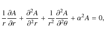
the right-handed orthogonal frame. The equation ![]() and the invariance of
and the invariance of ![]() in z implies that one can write the field
components as:
in z implies that one can write the field
components as: ![]() and
and ![]() ,
where A(x,y)
is the magnetic-flux function. The projection of field lines in a plane
orthogonal to the z axis is given by
isocontours of A(x,y).
The force-free condition implies
,
where A(x,y)
is the magnetic-flux function. The projection of field lines in a plane
orthogonal to the z axis is given by
isocontours of A(x,y).
The force-free condition implies
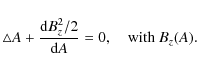
For an elliptical partial differential equation, such as Eq. (1), a boundary condition is generally required all around the region where the solution is searched for (otherwise the problem is ill posed, and, in particular, the solution is typically very sensitive to small modifications of the selected boundary values). The boundary of the flux rope is defined by the set of field lines having a given value of A(x,y). Without loss of generality, the origin of A can be set at the boundary, therefore
where xb,yb are the coordinates of the boundary (they are more precisely defined in Sect. 2.2). The maximal value of A(x,y) within the flux rope defines both the maximum amount of azimuthal magnetic flux and the position (x,y) of the flux rope center. Below we simply set this maximum as
since the azimuthal flux is later re-normalized to any desired value. Equations ((1), (2), (3)) have a non-singular solution for A(x,y) only for some Bz(A) functions (for example for a discrete series of Bz(A=1) values). This series of solutions are called resonant solutions (e.g. Morse & Feshbach 1953). This point is further explained in Sect. 2.4.
2.2 Boundary
The flux-rope
boundary can be generically defined by a closed parametric curve ![]() ,
where s is the variable defining the
position along the curve. The shape of the boundary influences the
shape of the field lines within the flux rope. However, with an
elliptic problem, such as given by Eq. (1), the small scale
deformations of the boundary are rapidly damped inside the volume (see
end of Sect. 3.2).
Conversely, knowing A(x,y)
in the deep interior of the flux rope, or on a cut through it (such as
with spacecraft observations) does not provide reliable information on
the spatial fluctuations of the boundary.
,
where s is the variable defining the
position along the curve. The shape of the boundary influences the
shape of the field lines within the flux rope. However, with an
elliptic problem, such as given by Eq. (1), the small scale
deformations of the boundary are rapidly damped inside the volume (see
end of Sect. 3.2).
Conversely, knowing A(x,y)
in the deep interior of the flux rope, or on a cut through it (such as
with spacecraft observations) does not provide reliable information on
the spatial fluctuations of the boundary.
We define a boundary shape that includes the main distortions
found in some MHD simulations (Sect. 1). In view of
previous works, an elliptical shape is a natural starting point. A
great variety of boundaries can be defined from the deformation of an
ellipse, but small-scale variations have only a local influence on the
force-free field, so we explore only large-scale deformations. To
minimize the number of free parameters, we restrict our analysis to
boundaries symmetric in the y direction
(orthogonal to the mean MC velocity). With these constraints, we derive
the following parametrization
where s ranges from s=0 at the front to s=1 at the back, and to s=2 to close the boundary at the front. The central size of this boundary in the x direction (at y=0) is normalized to 2, so that
A wider variety of boundaries can be analyzed with the method described below. However, Eq. (4) already provides a broad range of boundaries (see Figs. 3-5) with only two free parameters (a,b).
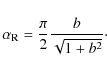
2.3 Linear force-free field
The Lundquist solution was, and still is, widely used for estimating the magnetic configuration of MCs crossed by a spacecraft (Sect. 1). We continue in the same line, by supposing a linear force-free magnetic field, i.e. with Bz(A) being a linear function of A. The axial component, Bz, is typically low at the boundary of MCs, so we restrict Bz(A) to an affine function of A. Therefore, Eq. (1) is simplified to
Equation (6)
is linear in A, therefore we can express A
as a linear combination of solutions. Since the Lundquist solution is
worked out in cylindrical coordinates, and since MCs are expected to be
not too far from being cylindrical (as a consequence of magnetic
tension), a set of functions can be searched for in cylindrical
coordinates. Then Eq. (6)
is rewritten as
where
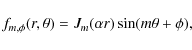
where Jm is the ordinary Bessel function of order m. Romashets & Vandas (2005) derived the magnetic components from a series of such functions, and determined the free coefficients by a fit to the magnetic data of some MCs (without imposing any boundary shape, different to the present study).
In practice, ![]() is approximated by a finite series of
is approximated by a finite series of ![]() .
This series satisfies Eq. (6)
exactly, but in most cases, it satisfies only approximately the
selected boundary condition (Eq. (4)). The precision
depends on both the number of functions kept in the series and on the
shape of the boundary. Except for m=0 (which
recovers the Lundquist solution), the
.
This series satisfies Eq. (6)
exactly, but in most cases, it satisfies only approximately the
selected boundary condition (Eq. (4)). The precision
depends on both the number of functions kept in the series and on the
shape of the boundary. Except for m=0 (which
recovers the Lundquist solution), the ![]() isocontour has a variety of non-circular shapes. So a combination of
several m modes can approximate a wide
variety of boundary shapes. Still, these modes have comparable sizes in
the x,y directions, so
this series of functions is not suited to approximate flat magnetic
configurations. The numerical results obtained with the set of
functions defined by Eq. (8)
confirm this. Moreover, some MCs have a magnetic field norm which is
nearly uniform in their cross-section (e.g., Vandas
et al. 2005). This indicates an approximate
magnetic-pressure balance, therefore a low magnetic tension, so a flat
magnetic configuration.
isocontour has a variety of non-circular shapes. So a combination of
several m modes can approximate a wide
variety of boundary shapes. Still, these modes have comparable sizes in
the x,y directions, so
this series of functions is not suited to approximate flat magnetic
configurations. The numerical results obtained with the set of
functions defined by Eq. (8)
confirm this. Moreover, some MCs have a magnetic field norm which is
nearly uniform in their cross-section (e.g., Vandas
et al. 2005). This indicates an approximate
magnetic-pressure balance, therefore a low magnetic tension, so a flat
magnetic configuration.
Another set of functions satisfying Eq. (6) can be derived in
Cartesian coordinates. We limit ourselves to functions even in y
since we are analyzing symmetric configurations (Sect. 2.2). The basic
functions are
where
2.4 Numerical solution with a linear force-free field
In practice,Therefore, A(x,y) is written as the series
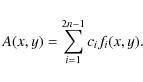
The coefficients ci are found so that A(x,y) best satisfy both the boundary condition of Eq. (2) and the normalization of Eq. (3).
Equations ((2),
(3), (6)) define an
eigenvalue problem that has a non singular solution inside the boundary
only for a discrete series of ![]() eigenvalues (e.g. Moon
& Spencer 1988; Morse & Feshbach 1953).
With A(x,y)
described by 2n-1 functions (Eq. (11)), we should set
A(xb,j,yb,j)=0
at 2n-1 boundary positions. Therefore, the
eigenvalues (e.g. Moon
& Spencer 1988; Morse & Feshbach 1953).
With A(x,y)
described by 2n-1 functions (Eq. (11)), we should set
A(xb,j,yb,j)=0
at 2n-1 boundary positions. Therefore, the ![]() values can be obtained by finding the zeros of
values can be obtained by finding the zeros of ![]() with i, j within [1,2n-1]
(e.g. Trott
2006; Morse
& Feshbach 1953, Chap. 3.5). For the
application to MCs, we are interested in the smallest
with i, j within [1,2n-1]
(e.g. Trott
2006; Morse
& Feshbach 1953, Chap. 3.5). For the
application to MCs, we are interested in the smallest ![]() eigenvalues, since for larger eigenvalues A(x,y)
and the magnetic field components also vanish inside the boundary, and
this case is not observed in MCs. We find that this method works well
for small values of n. However, as n
increases, the determinant computation involves the sum/subtraction of
a large number of terms, each being the product of 2n-1
functions (
fi(xb,j,yb,j)).
This implies that the determinant has huge variations with
eigenvalues, since for larger eigenvalues A(x,y)
and the magnetic field components also vanish inside the boundary, and
this case is not observed in MCs. We find that this method works well
for small values of n. However, as n
increases, the determinant computation involves the sum/subtraction of
a large number of terms, each being the product of 2n-1
functions (
fi(xb,j,yb,j)).
This implies that the determinant has huge variations with ![]() .
In particular, the determinant is very small when computed below the
first eigenvalue, while it reaches large values just above. The range
of variation can reach more than ten orders of magnitude. This huge
range does not facilitate the precise localization of the first zero of
the determinant, thus the determination of the first eigenvalue. We
conclude that this approach is effective only for small values
of n.
.
In particular, the determinant is very small when computed below the
first eigenvalue, while it reaches large values just above. The range
of variation can reach more than ten orders of magnitude. This huge
range does not facilitate the precise localization of the first zero of
the determinant, thus the determination of the first eigenvalue. We
conclude that this approach is effective only for small values
of n.
Another approach is to perform a least square fit of
Eq. (11)
to both nb
boundary points and to the normalization condition A(0,0)=1
(e.g. Trott 2006,
Chap. 1.2). With this method ![]() .
The condition A(0,0)=1 is only approximately
satisfied, but this can be corrected afterwards by multiplying A(x,y)
by a constant factor. More importantly, the condition A(xb,j,yb,j)=0
is only approximately satisfied at the nb
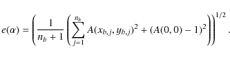
boundary points. We defined the mean error as
.
The condition A(0,0)=1 is only approximately
satisfied, but this can be corrected afterwards by multiplying A(x,y)
by a constant factor. More importantly, the condition A(xb,j,yb,j)=0
is only approximately satisfied at the nb
boundary points. We defined the mean error as
The advantage of this approach is that
A given non-zero value of a has a very
different implication for small and large b: with a
larger b, a larger a
value is needed to distort the flux rope significantly (see
Figs. 3-5). We choose to
scale a with ![]() in Figs. 2, 8-11, as the precision
of the method decreases significantly for
in Figs. 2, 8-11, as the precision
of the method decreases significantly for ![]() (Fig. 2).
(Fig. 2).
![\begin{figure}
\includegraphics[width=9cm, clip=]{12645f1.eps}\end{figure}](/articles/aa/full_html/2009/44/aa12645-09/img61.png)
|
Figure 1:
Evolution of the mean error, Eq. (12), as a function of
|
| Open with DEXTER | |
![\begin{figure}
\par\includegraphics[width=8.8cm]{12645f2.eps}
\end{figure}](/articles/aa/full_html/2009/44/aa12645-09/img62.png)
|
Figure 2:
Log-log plot of the smallest |
| Open with DEXTER | |
![\begin{figure}
\par\mbox{\includegraphics[width=4.4cm, clip=]{12645f3a.eps} ,
\includegraphics[width=4.4cm, clip=]{12645f3b.eps} }
\par
\end{figure}](/articles/aa/full_html/2009/44/aa12645-09/img63.png)
|
Figure 3:
Projected field lines orthogonal to the flux rope axis (isocontours
of A, left panels) and
isocontours of the magnetic field norm B (
right panels) for the first eigen solution (lowest |
| Open with DEXTER | |
![\begin{figure}
\par {\includegraphics[width=4.4cm, clip=]{12645f4a.eps} ,
\includegraphics[width=4.4cm, clip=]{12645f4b.eps} }
\par
\end{figure}](/articles/aa/full_html/2009/44/aa12645-09/img64.png)
|
Figure 4: Projected field lines (isocontours of A, left panels) and isocontours of the magnetic field norm B ( right panels). The boundaries are defined by Eq. (4) with an aspect ratio b=1. The drawing convention is the same as in Fig. 3. |
| Open with DEXTER | |
![\begin{figure}
\includegraphics[width=8.8cm, clip=]{12645f5.eps}
\end{figure}](/articles/aa/full_html/2009/44/aa12645-09/img65.png)
|
Figure 5: Projected field lines (isocontours of A, top panels) and isocontours of the magnetic field norm B ( bottom panels). The boundaries are defined by Eq. (4) with an aspect ratio b=3. The drawing convention is the same as in Fig. 3. |
| Open with DEXTER | |
3 Flux rope solutions
In this section we analyze the force-free solutions found. We start with a summary of previously known force-free solutions in order to compare them later with our results.3.1 Analytical solutions
The best-known solution is the Lundquist solution. It is
simply the first eigen-solution of a linear force-free field
with
Another simple solution can be found in Cartesian coordinates. This
geometry implies a rectangular boundary (of size ![]() with the same normalization as in Sect. 2.2). The
magnetic field is
with the same normalization as in Sect. 2.2). The
magnetic field is
with
This provides an order of magnitude estimate for the flux-rope characteristics, as shown below.
A third analytical solution for a linear force-free field with an elliptical boundary (particular case of Eq. (4) with a=0) was found by Vandas & Romashets (2003). Equation (6) was solved with elliptic cylindrical coordinates, one of the few coordinates system where Eq. (6) has separable solutions. For all b values, they found an analytical solution expressed with the even Mathieu function of zero order. While analytical, the explicit solution needs numerical computations that they achieved through a series expansion of the Mathieu function. We confirm all their derivations, including their numerical results (we computed them differently by using the Mathieu function inside the Mathematica software). We found only minor differences in the numerical results. We also found small differences when using the numerical method described in Sect. 2 (within the mean error found at the boundary shown in Fig. 2b).
3.2 Flux rope structure
The projections of field lines orthogonal to the flux rope axis are given by isocontour values of A(x,y). For a force-free field, they are also iso-values of the axial field Bz (Eq. (1)). Typically, field line projections inside the flux rope are more circular than the imposed boundary. This effect is stronger closer to the flux-rope center (Figs. 3-5). This is due to the balance of force, as follows. The sharper parts of the boundary impose a strong curvature, therefore a strong magnetic tension which reduces the field line bending inside the flux rope (see the regions around the corner of the rectangular boundary in Fig. 3a or the region with the most negative x-values forThe most important effect of the boundary on the core field is the aspect ratio (called b). The core field has approximately an elliptical shape with an aspect ratio closer to unity than the b value.
The next most important effect for the core field is a global
deformation of the boundary such as the effect induced by increasing |a|
in Eq. (4).
This is already a relatively weak effect for the field line shape
inside the flux-rope core, especially for large b values
(Figs. 3-5). For a larger
bending (i.e. a larger |a|), the magnetic
tension increases, so the magnetic field lines slightly shrink towards
the flux rope center (e.g. see the evolution of the ![]() isocontour with increasing |a| in
Fig. 5).
We notice that the distance
isocontour with increasing |a| in
Fig. 5).
We notice that the distance ![]() is preserved for each y value with
increasing |a|, so there is no compression
of the flux rope as |a| increases in all the
examples shown, and the observed shrinkage is not due to a compression
of the flux rope edges.
is preserved for each y value with
increasing |a|, so there is no compression
of the flux rope as |a| increases in all the
examples shown, and the observed shrinkage is not due to a compression
of the flux rope edges.
The bending of the flux rope introduces an asymmetry between the front and the back. Field lines in the front become flatter as |a| increases (Figs. 3-5). Even an inverse curvature (curved away from the flux-rope center) is present for the largest |a| values shown. This asymmetry is also present in the field strength, with the field being stronger in the front than in the back of the flux rope (Fig. 6). For a>0, symmetric results are obtained but such cases are usually not observed in MCs.
Next, let us consider a cut of the flux rope at y=0
in order to simulate observations made by a spacecraft. The deformation
of the boundary much less affects the direction of the magnetic field
than its norm. This is illustrated in Fig. 6 for one of
the spherical angles (![]() ), defining the direction of
), defining the direction of ![]() ,
and it is also true for the other angle
,
and it is also true for the other angle ![]() (
(
![]() ). This
result holds approximately also for values of |y/b|
not too large. Indeed, the isocontours of A
in Figs. 3-5 show that the
deformation of the projected field lines remains moderate if |a|
is increased. Since these A isocontours are
also isovalues of Bz,
the magnetic field direction in most of the flux rope is only slightly
affected if a is modified.
). This
result holds approximately also for values of |y/b|
not too large. Indeed, the isocontours of A
in Figs. 3-5 show that the
deformation of the projected field lines remains moderate if |a|
is increased. Since these A isocontours are
also isovalues of Bz,
the magnetic field direction in most of the flux rope is only slightly
affected if a is modified.
Inside the flux rope, small-scale distortions of the boundary
have even a weaker effect than the effect of |a|.
This can be shown by considering, for example, the field described by ![]() in cylindrical coordinates (Sect. 2.3). The
coefficient c gives the spatial-fluctuation
amplitude of the boundary (defined by
in cylindrical coordinates (Sect. 2.3). The
coefficient c gives the spatial-fluctuation
amplitude of the boundary (defined by ![]() ). Because
the Bessel functions behave as rm
near the origin, the deformation of the field lines decreases rapidly
with increasing m at a given
distance r inside the flux rope. We
conclude that the core of the flux rope is almost not affected by the
small-scale fluctuations of the flux rope boundary.
). Because
the Bessel functions behave as rm
near the origin, the deformation of the field lines decreases rapidly
with increasing m at a given
distance r inside the flux rope. We
conclude that the core of the flux rope is almost not affected by the
small-scale fluctuations of the flux rope boundary.
![\begin{figure}
\par\includegraphics[width=8.8cm, clip=]{12645f6.eps}
\end{figure}](/articles/aa/full_html/2009/44/aa12645-09/img87.png)
|
Figure 6:
Examples of magnetic field found across the flux rope along the x-axis
(y=0). B is the magnetic field
norm and |
| Open with DEXTER | |
3.3 Magnetic pressure at the boundary
The magnetic field strength (B) is always
maximum at the flux rope center (where Bx=By=0,
so where A, and therefore Bz(A),
have an extremum). However, this center is not necessarily at the
geometrical center of the shape defined by the boundary (see, e.g.,
Figs. 3-5). B
decreases faster toward the boundary where the boundary is extended
outward, or has a ``corner'', due to a stronger magnetic tension there
(Figs. 3-5). For
small b, high B values
are concentrated in a range of x almost
independently of y, while for large b values
this range is located rather at low |y| values.
Finally, the isocontours of B are
remarkably different from the field lines (isocontours of A)
with the exception of nearly circular contours for ![]() ,
,
![]() .
.
The magnetic pressure at the boundary strongly depends on the flux rope deformation (Fig. 7). Starting from the cylindrically symmetrical case (a=0,b=1), where the pressure is by construction uniform along the boundary, a small |a| already is sufficient to create a significant decrease of pressure on the lateral sides of the flux rope (Figs. 4d-f, 7b). For b<1 and a=0, the magnetic pressure is significantly higher on the sides of the flux rope (Fig. 3f), this effect being more pronounced for smaller b values. This effect competes with the flux rope bending (increasing |a|) to shift the pressure maximum/minimum along the boundary (Fig. 7a). For b>1, both an increasing b and |a| produce a lower magnetic pressure on the flux-rope sides (Figs. 5d-f, 7c).
The equilibrium of the flux rope with its surroundings is achieved by the total pressure balance at the boundary. Therefore, the above magnetic pressure computation gives the total pressure needed in the surrounding SW to achieve such a boundary shape (assuming a dominant magnetic pressure inside the flux rope). The asymmetry of the SW pressure between the front and the back of the flux rope can be due to encountered different SW, but in most cases it is plausibly due to the ram pressure due to the relative motion of the flux rope with respect to the surrounding SW.
![\begin{figure}
\par\includegraphics[width=8.5cm, clip=]{12645f7.eps}
\end{figure}](/articles/aa/full_html/2009/44/aa12645-09/img90.png)
|
Figure 7: Magnetic pressure along the flux rope boundary (Eq. (4)) normalized to the maximum pressure (located at the flux rope center). The coordinate s ranges from s=0 at the front, to s=1 at the back. |
| Open with DEXTER | |
Moreover, if the SW conditions permit such low pressure on the flux
rope sides, the force-free approximation is expected to be no longer
valid in these regions (near the most bent parts of the boundary). More
precisely, even with a plasma ![]() as low as 10-2 in the flux rope center, the
force-free approximation is no longer valid in the regions where the
relative magnetic pressure reaches few 10-2 in
Fig. 7
(supposing a nearly uniform plasma pressure). Such regions are expected
to be advected with the plasma flow (in the absence of reconnection),
so that the extended parts of the flux rope are expected to be swept
away by the SW. Reconnection with the encountered SW magnetic field is
also expected; it will further contribute to remove these extended
parts. It remains a strong core with an elliptical-like shape. This
core field is expected to keep its identity while traveling in the SW
(unless there is a large amount of magnetic flux reconnected with the
overtaken SW).
as low as 10-2 in the flux rope center, the
force-free approximation is no longer valid in the regions where the
relative magnetic pressure reaches few 10-2 in
Fig. 7
(supposing a nearly uniform plasma pressure). Such regions are expected
to be advected with the plasma flow (in the absence of reconnection),
so that the extended parts of the flux rope are expected to be swept
away by the SW. Reconnection with the encountered SW magnetic field is
also expected; it will further contribute to remove these extended
parts. It remains a strong core with an elliptical-like shape. This
core field is expected to keep its identity while traveling in the SW
(unless there is a large amount of magnetic flux reconnected with the
overtaken SW).
![\begin{figure}
\par\includegraphics[width=8.5cm, clip=]{12645f8ab.eps}
\includegraphics[width=8.5cm, clip=]{12645f8c.eps}
\end{figure}](/articles/aa/full_html/2009/44/aa12645-09/img91.png)
|
Figure 8: Modification with b of the magnetic flux and helicity contained in the flux rope(per unit length along the axial direction). a) The maximum magnetic field strength is set to unity, b) the axial flux is normalized to the azimuthal flux, and c) the helicity is normalized to the product of the fluxes. |
| Open with DEXTER | |
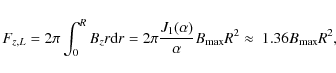
3.4 Magnetic flux
The axial flux of the Lundquist solution, Eq. (13), is
where the two first expressions are general (valid for any
where L is the axial length of the flux tube. The ratio of fluxes is
The axial flux within a rectangular cross-section is computed from Eq. (14)
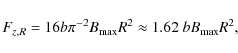
where we keep the same field and size scaling (the cross-section size is
where
At the limit of a small aspect-ratio b, this flux ratio is constant, while it increases linearly with b in the limit of large b (Fig. 8b).
With the same maximum field strength and maximum extension in
both x and y directions, the
axial flux obtained with the boundary defined by Eq. (4) is always lower
than the axial flux obtained with the rectangular boundary
(Fig. 8a).
This is an expected result since the area defined by Eq. (4) is slightly
smaller than the area of the rectangular boundary. The difference
increases as the aspect ratio (b) departs
from unity. This is a consequence of the shrinkage of the field lines
as the core has a lower aspect ratio for an elliptical than for a
rectangular boundary (Fig. 3-5). This
difference reaches a factor about 2 (shift of ![]() 0.3 in
0.3 in ![]() scale) both for
scale) both for ![]() and
and ![]() 10.
The bending of the flux-rope cross-section, so increasing |a|,
has a much weaker effect (Fig. 8a).
10.
The bending of the flux-rope cross-section, so increasing |a|,
has a much weaker effect (Fig. 8a).
The azimuthal flux, ![]() ,
is also an increasing function of b
because
,
is also an increasing function of b
because ![]() is a decreasing function of b
(Fig. 2).
Therefore, the ratio
is a decreasing function of b
(Fig. 2).
Therefore, the ratio ![]() has a weaker dependence on b than Fz
(Fig. 8b).
has a weaker dependence on b than Fz
(Fig. 8b).
![]() has a nearly linear dependence on b in a
log-log plot, for the whole range of a
explored. This contrasts with the result obtained with the rectangular
cross-section. In the range 0.1<b<10,
we deduced
has a nearly linear dependence on b in a
log-log plot, for the whole range of a
explored. This contrasts with the result obtained with the rectangular
cross-section. In the range 0.1<b<10,
we deduced ![]() ,
the lower bound being given by the Lundquist solution and the upper
bound being an approximation both for low and high b values.
,
the lower bound being given by the Lundquist solution and the upper
bound being an approximation both for low and high b values.
3.5 Magnetic helicity
An efficient way to compute the magnetic helicity of the
field ![]() within a volume
within a volume ![]() is to split the field
is to split the field ![]() into two parts, as
into two parts, as ![]() ,
where
,
where ![]() is fully contained inside
is fully contained inside ![]() ,
and
,
and ![]() has the same distribution as
has the same distribution as ![]() on the boundary of
on the boundary of ![]() (Berger 2003). For an
element of length L of a flux rope, a
simple choice for
(Berger 2003). For an
element of length L of a flux rope, a
simple choice for ![]() and
and ![]() is the azimuthal (
is the azimuthal (
![]() )
and axial (
)
and axial (
![]() )
field components, respectively
)
field components, respectively
where
where the first expression is general, while
However, Eq. (23)
is not convenient to compute the helicity for a general cross-section
shape, since one first needs to compute
![]() by integration of Bz.
Equation (22)
can be transformed with the vector identity
by integration of Bz.
Equation (22)
can be transformed with the vector identity
![]() where
where ![]() and
and ![]() .
The surface integral on the flux rope boundary,
.
The surface integral on the flux rope boundary, ![]() ,
vanishes if Az=A=0.
This is a particular gauge for the vector potential, that we have
already selected in Sect. 2.2. Therefore,
with A=0 at the flux rope boundary, Eq. (22) can be
rewritten as
,
vanishes if Az=A=0.
This is a particular gauge for the vector potential, that we have
already selected in Sect. 2.2. Therefore,
with A=0 at the flux rope boundary, Eq. (22) can be
rewritten as
This integral is much easier to compute than the one in Eq. (23), since it involves only scalar quantities that are direct outputs of the model.
With Eq. (25),
the helicity of a flux rope with a rectangular cross-section is easily
computed as
For b=1, a flux rope with a square cross-section contains only 28% more helicity than a flux rope with a circular cross-section. This is only slightly above the ratio obtained above for the axial flux (20%, Sect. 3.4).
As for Fz, magnetic helicity is greater for the rectangular cross-section, and this difference is larger for b values far from 1 (both smaller and larger values, Fig. 8a). Also, H(b) is a steeper function than Fz(b) for low b values, while H(b) and Fz(b) have a comparable slope for large b values.
Magnetic helicity quantifies how much the axial and azimuthal
fluxes are interlinked. A useful quantity is the normalized helicity (
![]() ); it is an average Gauss
linking number (Berger &
Field 1984). It is independent of b for a
rectangular cross-section (
); it is an average Gauss
linking number (Berger &
Field 1984). It is independent of b for a
rectangular cross-section (
![]() ),
a value just below the result of the Lundquist solution (
),
a value just below the result of the Lundquist solution (
![]() ).
With the boundary defined by Eq. (4),
).
With the boundary defined by Eq. (4), ![]() depends only weakly on both a and b
(
depends only weakly on both a and b
(
![]() )
over the large range explored for b
(Fig. 8c).
Therefore, the magnetic helicity contained in these flux ropes is
mainly defined by their magnetic flux (the mean flux linkage being
almost constant). We anticipate that this result could be extended to a
much broader ensemble of boundary shapes than those defined by
Eq. (4).
)
over the large range explored for b
(Fig. 8c).
Therefore, the magnetic helicity contained in these flux ropes is
mainly defined by their magnetic flux (the mean flux linkage being
almost constant). We anticipate that this result could be extended to a
much broader ensemble of boundary shapes than those defined by
Eq. (4).
4 Estimation of the boundary shape from B along a 1D cut of the flux rope
In this section, we analyze the magnetic field profile computed along a cut of the flux rope along the x direction (at a fixed y value). The aim is to provide a first step toward the analysis of in-situ data by identifying the characteristics of the field profile that permit us to determine approximately the parameters of the model that is most compatible with the observations. The final determination of the parameters will be realized by a least square fit to the data in a subsequent work. However, this procedure is not a trivial task due to the number of free parameters involved. The fitting method will largely benefit from the following approximate determination of the parameters since the iteration involved in the fitting can be initiated closer to the best solution (i.e., starting the iteration from a ``good'' seed). This will speed up the convergence towards the global minimum of the function defined as the distance of the model to the observations, and even more importantly, it will limit the possibility of converging to a local minimum, rather than the global minimum (i.e., the risk to end up at a false solution).
4.1 Aspect ratio
The aspect ratio, b, of the boundary has a
strong effect on the field-line curvature, so on the contribution of
the magnetic tension. Together with the force-free balance, it implies
that b has a strong influence on the
distribution of the field strength B inside
the flux rope (Figs. 3-5). More
precisely, cuts across the flux rope parallel to the x-axis,
at a fixed ![]() ,
have a clearly peaked B(x)
profile for low b values, and this profile
becomes flatter as b increases
(Fig. 6).
,
have a clearly peaked B(x)
profile for low b values, and this profile
becomes flatter as b increases
(Fig. 6).
We take advantage of the above property to present a method to
estimate b from B(x).
Several attempts have been investigated to characterize the B(x) profile
as a function of b, for example by
computing the mean curvature of the B(x) profile.
However, this curvature depends on ![]() and on the size of the x-interval crossed. From these explorations, we
find that this approach is suited only to relatively low impact
parameters. In our exploration of the different possibilities, we
select the option which has the least dependence on other parameters
(such as the y and a values).
We also define global quantities, rather than local ones, to have less
influence of local perturbations in future applications to
observations.
and on the size of the x-interval crossed. From these explorations, we
find that this approach is suited only to relatively low impact
parameters. In our exploration of the different possibilities, we
select the option which has the least dependence on other parameters
(such as the y and a values).
We also define global quantities, rather than local ones, to have less
influence of local perturbations in future applications to
observations.
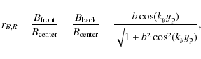
The best estimator of the parameter b we
found is the ratio
where the averaging is done over a fraction f of the x-extension of the analyzed B profile.
Figure 9
demonstrates that rB
has a well defined variation with b. The saturation
of rB,
close to 0 and 1 for small and large b values,
respectively, is intrinsic to the force-free balance (Sect. 3.2). As a
consequence, the estimation of b is less
accurate for small and large b values.
Next, rB
is weakly dependent on a, so on the bending
of the flux rope. This is so because rB
is defined by an average of the front and back field. rB
is also weakly dependent on ![]() ,
a result coming from the global force balance (Sect. 3.2). Finally,
since rB
is defined as a function of B, this implies
that rB
is explicitly independent of the estimation of the axis orientation.
However, there is still an implicit dependence since the determination
of the MC boundaries is more accurate in the MC frame (Dasso et al. 2006).
,
a result coming from the global force balance (Sect. 3.2). Finally,
since rB
is defined as a function of B, this implies
that rB
is explicitly independent of the estimation of the axis orientation.
However, there is still an implicit dependence since the determination
of the MC boundaries is more accurate in the MC frame (Dasso et al. 2006).
![\begin{figure}
\par\includegraphics[width=8.8cm, clip=]{12645f9.eps}
\end{figure}](/articles/aa/full_html/2009/44/aa12645-09/img138.png)
|
Figure 9:
Evolution of magnetic field ratio, rB,
defined by Eq. (27),
as a function of |
| Open with DEXTER | |
The above numerical results could be directly used to estimate the
aspect ratio b using the measured value of rB
(by interpolating a table of values). However, it is more practical to
derive an analytical approximation. This task is largely facilitated by
the dominant dependence of rB
on b. As a guide we compare with the result
obtained with a rectangular cross-section. From Eq. (14), we find:
where
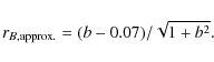
This provides a relatively good approximation for the numerical results for
4.2 Orientation of the flux-rope axis
A classical method to determine the local axis orientation of
an MC is the minimum variance method (MV, see e.g., Burlaga
et al. 1982; Sonnerup & Cahill 1967).
It is based on the different behavior of the axial and the two
orthogonal components of the magnetic field which is expected, since an
MC has a flux rope structure. The method finds the directions where the
magnetic field has the lowest and the highest variance (the third
direction, with an intermediate variance, being orthogonal). The MV
requires that the three variance values are well separated, a condition
generally met in MCs. Thus, the MV provides approximately the
directions x,y,z
used above (we recall that the flux rope is supposed to move away from
the Sun along ![]() ).
).
The MV was extensively used to find the local axis of MCs
(e.g., Gulisano
et al. 2007; Bothmer & Schwenn 1998,
and references therein). It provides more accurate results when it is
applied to a normalized time series ![]() .
It was compared to other methods, in most cases successfully, with
typical differences between the methods of the order of
.
It was compared to other methods, in most cases successfully, with
typical differences between the methods of the order of
![]() .
The most important deviation in the orientation is produced by changing
the MC boundaries (Dasso
et al. 2006). Also the systematic error in the
orientation increases with the impact parameter,
.
The most important deviation in the orientation is produced by changing
the MC boundaries (Dasso
et al. 2006). Also the systematic error in the
orientation increases with the impact parameter, ![]() .
However, the tests of Gulisano
et al. (2007) with Lundquist's test fields have
shown a deviation of only
.
However, the tests of Gulisano
et al. (2007) with Lundquist's test fields have
shown a deviation of only ![]()
![]() for
for ![]() %
of the MC radius and of
%
of the MC radius and of ![]()
![]() for
for ![]() as high as
as high as ![]() 90%
of the MC radius.
90%
of the MC radius.
The results of Sect. 3.2 show that
the orientation of the magnetic field is weakly affected by the shape
of the cross-section. This is true for low impact parameters (see the
case ![]() in Fig. 6b,d),
as well as in about the half of the flux rope (as can be deduced
qualitatively from Figs. 3-5, see
Sect. 3.2).
Therefore, we expect that the results previously obtained in tests of
cylindrical models are approximately valid also for flux ropes with
distorted cross-section.
in Fig. 6b,d),
as well as in about the half of the flux rope (as can be deduced
qualitatively from Figs. 3-5, see
Sect. 3.2).
Therefore, we expect that the results previously obtained in tests of
cylindrical models are approximately valid also for flux ropes with
distorted cross-section.
The main advantage of the MV method is that it does not
introduce an a priori on the detailed magnetic configuration of the
flux rope (e.g., the distribution of the twist). The small dependence
of the time series ![]() on the cross-section shape further justifies the use of the MV. This
provides an estimation of the MC frame, defined by the x,y,z directions,
in which the data are transformed for the next steps.
on the cross-section shape further justifies the use of the MV. This
provides an estimation of the MC frame, defined by the x,y,z directions,
in which the data are transformed for the next steps.
| Figure 10:
Estimation of |
|
| Open with DEXTER | |
4.3 Impact parameter
Global quantities, such as magnetic flux and helicity, are
extensive quantities, i.e. they depend on the MC size. In order to
estimate the true size of the flux rope, it is therefore important to
relate the x extension measured along the
flux-rope crossing to its value for a central crossing (where B
is maximum). This is realized by estimating ![]() .
.
The ![]() position of the cut affects the three components of
position of the cut affects the three components of ![]() ,
as can be deduced from Figs. 3-5. As for the
determination of b above we search for the
best way to estimate
,
as can be deduced from Figs. 3-5. As for the
determination of b above we search for the
best way to estimate ![]() .
Gulisano et al. (2007)
have used
.
Gulisano et al. (2007)
have used ![]() normalized to the central field strength,
normalized to the central field strength, ![]() ,
which was deduced by fitting the Lundquist solution to the data. They
derived a quadratic relationship between
,
which was deduced by fitting the Lundquist solution to the data. They
derived a quadratic relationship between ![]() and
and ![]() for a magnetic field defined by the Lundquist solution. Here, we extend
this approach, by computing
for a magnetic field defined by the Lundquist solution. Here, we extend
this approach, by computing
where the averages are computed over the full crossing of the flux rope (at a given
Figure 10
shows that rBx
has a well defined variation with ![]() ,
but that it also depends on b, and to a
lesser extent on a. Moreover, since Bx
is involved, rBx
is also affected by the determination of the local MC frame
(Sect. 4.2).
With a rough estimation, we find
,
but that it also depends on b, and to a
lesser extent on a. Moreover, since Bx
is involved, rBx
is also affected by the determination of the local MC frame
(Sect. 4.2).
With a rough estimation, we find ![]() .
More precisely, the proportionality coefficient depends weakly on b,
with a value
.
More precisely, the proportionality coefficient depends weakly on b,
with a value ![]() 0.7
for
0.7
for ![]() ,
and
,
and ![]() 1.7
for
1.7
for ![]() ,
so the above affine relation can be systematically biased, up to 40%,
for a very small or for a very large aspect ratio. A better
approximation is:
,
so the above affine relation can be systematically biased, up to 40%,
for a very small or for a very large aspect ratio. A better
approximation is:
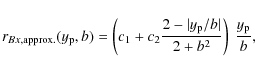
where c1 and c2 are slightly function of
Finally, the estimation of ![]() permits us to estimate the x extension of a central
crossing from the measure of
permits us to estimate the x extension of a central
crossing from the measure of ![]() ,
as deduced from the observed velocity, from the determination of the
boundaries and from the axial orientation of the MC. With a boundary
parametrized by Eq. (4),
this step does not depend on a (as
,
as deduced from the observed velocity, from the determination of the
boundaries and from the axial orientation of the MC. With a boundary
parametrized by Eq. (4),
this step does not depend on a (as ![]() is independent of a for a given
is independent of a for a given ![]() value).
value).
![\begin{figure}
\par\includegraphics[width=8.8cm, clip=]{12645f11.eps}
\end{figure}](/articles/aa/full_html/2009/44/aa12645-09/img167.png)
|
Figure 11:
Evolution of the asymmetry ratio |
| Open with DEXTER | |
4.4 Bending
A global bending of the flux rope has a relatively weak effect on the magnetic field (Figs. 3-5). The strongest effect is present on the By component as the front field is increasing with more negative a values, while the opposite occurs in the back of the flux rope (for not too large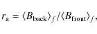
where the averaging is done over a fraction f of the x-extension of the analyzed B profile. As for Eq. (27), we select f=0.2.
![]() strongly depends on a, but only for b
lower than a few units (Fig. 11). Indeed, we show
curves with fixed values of
strongly depends on a, but only for b
lower than a few units (Fig. 11). Indeed, we show
curves with fixed values of ![]() ,
which implies an increasing value of a with b.
Therefore, equivalent curves, with a fixed value for a,
would show an even lower dependence on a for b>1.
Indeed, when
,
which implies an increasing value of a with b.
Therefore, equivalent curves, with a fixed value for a,
would show an even lower dependence on a for b>1.
Indeed, when ![]() ,
a comparable to b is
required in order that magnetic tension modifies significantly the
otherwise flat B(x)
profile (Figs. 5-6). The choice
of the scaling of a with
,
a comparable to b is
required in order that magnetic tension modifies significantly the
otherwise flat B(x)
profile (Figs. 5-6). The choice
of the scaling of a with ![]() was guided by numerical errors (see the end of Sect. 2.4). However,
values of a larger than
was guided by numerical errors (see the end of Sect. 2.4). However,
values of a larger than ![]() are expected to be unphysical (in particular they were not found in MHD
simulations, e.g., Riley
et al. 2003; Manchester
et al. 2004), so we claim that Fig. 11 represents a
sufficiently broad range of the parameter space which covers most of
the observed MC configurations.
are expected to be unphysical (in particular they were not found in MHD
simulations, e.g., Riley
et al. 2003; Manchester
et al. 2004), so we claim that Fig. 11 represents a
sufficiently broad range of the parameter space which covers most of
the observed MC configurations.
![]() does not only depend on a, but also strongly on b,
as well as on
does not only depend on a, but also strongly on b,
as well as on ![]() as shown in Fig. 11.
Moreover, these dependences are coupled (the curves evolved
significantly with the three parameters), therefore we do not present
an analytical approximation (which would be cumbersome). However,
with b and
as shown in Fig. 11.
Moreover, these dependences are coupled (the curves evolved
significantly with the three parameters), therefore we do not present
an analytical approximation (which would be cumbersome). However,
with b and ![]() approximatively determined with the previous steps (Sects. 4.1, 4.3), a
can be estimated from the interpolation of a table of
approximatively determined with the previous steps (Sects. 4.1, 4.3), a
can be estimated from the interpolation of a table of ![]() values.
values.
These estimations can be refined by fitting the model developed in Sect. 2 to the data, with the initial parameters set to the above estimations. The purpose of the next paper will be to apply this new technique to a set of MCs. The difference between the initial parameters and the fitted ones will provide an estimation of the precision of the above estimations when applied to data.
5 Conclusions
The present work is motivated by the need for a magnetic model in order to derive the magnetic configuration of MCs from local measurements provided by spacecraft. The model should be able to compute a large variety of magnetic configurations, as broad as possible, but also the parameters of the model should be well defined from the observations.
To develop the above goal, we generalized the Lundquist solution, obtained in cylindrical symmetry, the MC boundary having a broad range of shapes. We express the solution with a series of functions satisfying the linear force-free equations. Such a development in series usually involve a large number of free parameters (the multiplicative coefficients of the functions in the series). Here we limit the freedom of the model by imposing the shape of the MC boundary (depending on few parameters). Moreover, it defines a well posed problem. For a given boundary shape, the internal magnetic-field solution is unique. This procedure provides a solution accurate enough over a broad range of aspect ratios of the flux rope cross-section (typically 0.1 to 10). While the boundary shape can be more general with this method, we limit our report to the boundary deformations which dominantly affect the observed magnetic field. Other deformations have a lower effect inside the flux rope, in particular on its core, and only future studies will be able to tell if some of these deformations could be estimated accurately enough from the data.
The physical origin of the cross-section deformation is the flux rope interaction with its surrounding SW. In particular, during the MC travel through the heliosphere, different parts of the MC boundary could be in contact with different parcels of SW having different pressure, therefore changing the original shape of the MC. These changes of the MC boundary drive a re-configuration of the internal magnetic field, in a similar way to the global expansion of MCs proposed by Démoulin & Dasso (2009). Thus, the shape of the MC boundary given by Eq. (4) can be interpreted as a consequence of the interaction of the flux rope with its environment. We found that a flat or/and bent flux-rope cross section requires a large gradient of the total pressure along the MC boundary (Fig. 7). Such a large gradient of pressure is unlikely to be present around MCs outside the interacting regions between two types of SW.
The most important deformation is a global elongation of the flux-rope cross-section. It is characterized by the aspect ratio (b), defined by the ratio of the dimension across to the one along the spacecraft trajectory projected orthogonally to the MC axis. Simulating the crossing of the flux rope by a spacecraft, we find that, for low b values, the magnetic field strength peaks inside the flux rope, while it becomes flatter as b increases. We quantify this property so that b can be estimated from the magnetic data collected across a MC. We also confirm the results of Vandas & Romashets (2003) who derived an analytical solution of a linear force-free field contained inside an elliptical boundary. We find that the configuration of the core inherits the oblate shape of the boundary but with a significantly lower aspect ratio, in agreement with previous observations (e.g., Dasso et al. 2005a; Liu et al. 2008; Möstl et al. 2009).
The next deformation in importance is the global bending of the flux rope coming from its interaction with surrounding SW streams (see refs. in Sect. 1). The symmetric bending mode (Figs. 3-5) can significantly affect the magnetic tension, therefore also the distribution of the field strength. With a bending in the direction of the MC propagation, a stronger field in the front than in the back is present, as frequently observed in MCs. Such asymmetry can also come from the temporal evolution of the magnetic field as the observations of the front and back are shifted in time (this effect is called the ``aging effect''). However, this effect can be corrected, and it is usually not the main cause of the observed asymmetry between the front and back of MCs (Démoulin et al. 2008). Moreover, even removing the aging effect, a front/back asymmetry can still be observed in some MCs (Mandrini et al. 2007; Dasso et al. 2007). Finally, we find that the deformation of the flux-rope core decreases with higher spatial frequency deformations of the boundary.
We next analyzed the results of the model with the perspective of applying it to MC data. In particular we search for the best way to have an efficient first estimation of the model parameters. This step is important as the parameter space to explore is large, and our previous experience of a direct fit of a simpler model to the data has shown us that a direct fit does not always converge to the correct solution. This consideration is even more important as the number of free parameters is larger in the present model. We also verify that the magnetic field taken only on a linear cut through the flux rope was sensitive enough to determine the parameters. We find that this is true for all parameter, when located in the expected physical range. The main limitation is the measurent of the bending (so a) for large aspect ratio (b).
In previous studies, the determination of the MC axis was realized mainly with the minimum variance or/and with a fit of the Lundquist model. We find that the distortions of the MC boundary shape mainly affect the magnetic field strength, but only weakly its direction. Therefore, the MC axis direction found in previous studies will remain weakly affected by applying the present new model. It implies that the local magnetic frame is relatively well defined. This is an important result to determine accurately the locations of the MC boundaries, as well as the impact parameter. We find a direct relationship between the impact parameter and the mean magnetic-field component present along the projection of the spacecraft trajectory orthogonally to the MC axis. We conclude that all the free parameters of the model can be constrained, and so determined, from a time series of a measured magnetic field within a MC.
Finally, we plan to study how much global quantities, such as magnetic flux and helicity, are modified in comparison with their previous estimations using the Lundquist field on MCs. Our model shows that the estimation of the aspect ratio (b) is the most important parameter of the MC cross-section for these global quantities. Other boundary deformation, such as the global bending (a), have a much smaller effect on the global quantities. We also found that the magnetic helicity, normalized by the product of the axial and azimuthal fluxes, is very weakly dependent on the boundary shape (at least with a linear force-free field).
AcknowledgementsWe thank Tibor Török for reading carefully, and so, improving the manuscript. The authors acknowledge financial support from ECOS-Sud through their cooperative science program (No. A08U01). This work was partially supported by the Argentinean grants: UBACyT X425 and PICT 2007-00856 (ANPCyT). S.D. is member of the Carrera del Investigador Científico, CONICET.
References
- Berger, M. A., & Field, G. B. 1984, J. Fluid. Mech., 147, 133 [CrossRef] [NASA ADS]
- Berger, M. A. 2003, in Advances in Nonlinear Dynamics, 345
- Botha, G. J. J., & Evangelidis, E. A. 2004, MNRAS, 350, 375 [CrossRef] [NASA ADS]
- Bothmer, V., & Schwenn, R. 1998, Annales Geophys., 16, 1 [CrossRef] [NASA ADS]
- Burlaga, L. F. 1988, J. Geophys. Res., 93, 7217 [CrossRef] [NASA ADS]
- Burlaga, L. F. 1995, Interplanetary magnetohydrodynamics (New York: Oxford University Press)
- Burlaga, L. F., & Behannon, K. W. 1982, Sol. Phys., 81, 181 [CrossRef] [NASA ADS]
- Burlaga, L., Sittler, E., Mariani, F., & Schwenn, R. 1981, J. Geophys. Res., 86, 6673 [CrossRef] [NASA ADS]
- Burlaga, L. F., Klein, L., Sheeley, Jr., N. R., et al. 1982, Geophys. Res. Lett., 9, 1317 [CrossRef] [NASA ADS]
- Cid, C., Hidalgo, M. A., Nieves-Chinchilla, T., Sequeiros, J., & Viñas, A. F. 2002, Sol. Phys., 207, 187 [CrossRef] [NASA ADS]
- Dasso, S., Mandrini, C. H., Démoulin, P., & Farrugia, C. J. 2003, J. Geophys. Res., 108, 1362 [CrossRef]
- Dasso, S., Gulisano, A. M., Mandrini, C. H., & Démoulin, P. 2005a, Adv. Space Res., 35, 2172 [CrossRef] [NASA ADS]
- Dasso, S., Mandrini, C. H., Démoulin, P., Luoni, M. L., & Gulisano, A. M. 2005b, Adv. Space Res., 35, 711 [CrossRef] [NASA ADS]
- Dasso, S., Mandrini, C. H., Démoulin, P., & Luoni, M. L. 2006, A&A, 455, 349 [EDP Sciences] [CrossRef] [NASA ADS]
- Dasso, S., Nakwacki, M. S., Démoulin, P., & Mandrini, C. H. 2007, Sol. Phys., 244, 115 [CrossRef] [NASA ADS]
- Démoulin, P. 2008, Annales Geophys., 26, 3113 [NASA ADS]
- Démoulin, P., & Dasso, S. 2009, A&A, 498, 551 [EDP Sciences] [CrossRef] [NASA ADS]
- Démoulin, P., Nakwacki, M. S., Dasso, S., & Mandrini, C. H. 2008, Sol. Phys., 250, 347 [CrossRef] [NASA ADS]
- Farrugia, C. J., Janoo, L. A., Torbert, R. B., et al. 1999, in Solar Wind Nine, ed. S. R. Habbal, R. Esser, J. V. Hollweg, & P. A. Isenberg, AIP Conf. Proc., 471, 745
- Feng, H. Q., Wu, D. J., & Chao, J. K. 2007, J. Geophys. Res., 112, A02102 [CrossRef]
- Gold, T., & Hoyle, F. 1960, MNRAS, 120, 89 [NASA ADS]
- Gulisano, A. M., Dasso, S., Mandrini, C. H., & Démoulin, P. 2005, J. Atmosph. Sol.-Terrestr. Phys., 67, 1761 [CrossRef] [NASA ADS]
- Gulisano, A. M., Dasso, S., Mandrini, C. H., & Démoulin, P. 2007, Adv. Space Res., 40, 1881 [CrossRef] [NASA ADS]
- Hidalgo, M. A. 2003, J. Geophys. Res., 108, 1320 [CrossRef]
- Hu, Q., & Sonnerup, B. U. Ö. 2002, J. Geophys. Res., 107, 1142 [CrossRef]
- Hu, Q., Smith, C. W., Ness, N. F., & Skoug, R. M. 2005, J. Geophys. Res., 110, A09S [CrossRef]03
- Kilpua, E. K. J., Liewer, P. C., Farrugia, C., et al. 2009, Sol. Phys., 254, 325 [CrossRef] [NASA ADS]
- Klein, L. W., & Burlaga, L. F. 1982, J. Geophys. Res., 87, 613 [CrossRef] [NASA ADS]
- Leitner, M., Farrugia, C. J., Möstl, C., et al. 2007, J. Geophys. Res., 112, A06113 [CrossRef]
- Lepping, R. P., Burlaga, L. F., & Jones, J. A. 1990, J. Geophys. Res., 95, 11957 [CrossRef] [NASA ADS]
- Lepping, R. P., Berdichevsky, D. B., Szabo, A., Arqueros, C., & Lazarus, A. J. 2003, Sol. Phys., 212, 425 [CrossRef] [NASA ADS]
- Liu, Y., Luhmann, J. G., Huttunen, K. E. J., et al. 2008, ApJ, 677, L133 [CrossRef] [NASA ADS]
- Lundquist, S. 1950, Ark. Fys., 2, 361
- Lynch, B. J., Zurbuchen, T. H., Fisk, L. A., & Antiochos, S. K. 2003, J. Geophys. Res., 108, 1239 [CrossRef]
- Manchester, W. B. I., Gombosi, T. I., Roussev, I., et al. 2004, J. Geophys. Res., 109, A02107 [CrossRef]
- Mandrini, C. H., Pohjolainen, S., Dasso, S., et al. 2005, A&A, 434, 725 [EDP Sciences] [CrossRef] [NASA ADS]
- Mandrini, C. H., Nakwacki, M., Attrill, G., et al. 2007, Sol. Phys., 244, 25 [CrossRef] [NASA ADS]
- Moon, P., & Spencer, D. E. 1988, Field Theory Handbook, Including Coordinate Systems, Differential Equations, and Their Solutions, 2nd ed. (New York: Springer-Verlag)
- Morse, P. M., & Feshbach, H. 1953, Methods of Theoretical Physics, Part I (New York: McGraw-Hill)
- Möstl, C., Farrugia, C. J., Biernat, H. K., et al. 2009, Sol. Phys., 256, 427 [CrossRef] [NASA ADS]
- Mulligan, T., Russell, C. T., Anderson, B. J., et al. 1999, in Solar Wind Nine, ed. S. R. Habbal, R. Esser, J. V. Hollweg, & P. A. Isenberg, AIP Conf. Proc., 471, 689
- Owens, M. J., Merkin, V. G., & Riley, P. 2006, J. Geophys. Res., 111, A03104 [CrossRef]
- Riley, P., Linker, J. A., Mikic, Z., et al. 2003, J. Geophys. Res., 108, 1272 [CrossRef]
- Riley, P., Linker, J. A., Lionello, R., et al. 2004, J. Atmos. Sol. Terr. Phys., 66, 1321 [CrossRef] [NASA ADS]
- Romashets, E. P., & Vandas, M. 2005, Adv. Spa. Res., 35, 2167 [CrossRef] [NASA ADS]
- Sonnerup, B. U., & Cahill, L. J. 1967, J. Geophys. Res., 72, 171 [CrossRef] [NASA ADS]
- Trott, M. 2006, The Mathematica Guidebook for Numerics (Springer)
- Vandas, M., & Romashets, E. P. 2003, A&A, 398, 801 [EDP Sciences] [CrossRef] [NASA ADS]
- Vandas, M., Odstrcil, D., & Watari, S. 2002, J. Geophys. Res., 107, 1236 [CrossRef]
- Vandas, M., Romashets, E. P., & Watari, S. 2005, Planet. Space Sci., 53, 19 [CrossRef] [NASA ADS]
- Vladimirov, V. S. 1984, Equations of Mathematical Physics (Mir, Moscow)
- Wu, C.-C., & Lepping, R. P. 2007, Sol. Phys., 242, 159 [CrossRef] [NASA ADS]
All Figures
|
|
Figure 1:
Evolution of the mean error, Eq. (12), as a function of
|
| Open with DEXTER | |
| In the text | |
|
|
Figure 2:
Log-log plot of the smallest |
| Open with DEXTER | |
| In the text | |
|
|
Figure 3:
Projected field lines orthogonal to the flux rope axis (isocontours
of A, left panels) and
isocontours of the magnetic field norm B (
right panels) for the first eigen solution (lowest |
| Open with DEXTER | |
| In the text | |
|
|
Figure 4: Projected field lines (isocontours of A, left panels) and isocontours of the magnetic field norm B ( right panels). The boundaries are defined by Eq. (4) with an aspect ratio b=1. The drawing convention is the same as in Fig. 3. |
| Open with DEXTER | |
| In the text | |
|
|
Figure 5: Projected field lines (isocontours of A, top panels) and isocontours of the magnetic field norm B ( bottom panels). The boundaries are defined by Eq. (4) with an aspect ratio b=3. The drawing convention is the same as in Fig. 3. |
| Open with DEXTER | |
| In the text | |
|
|
Figure 6:
Examples of magnetic field found across the flux rope along the x-axis
(y=0). B is the magnetic field
norm and |
| Open with DEXTER | |
| In the text | |
|
|
Figure 7: Magnetic pressure along the flux rope boundary (Eq. (4)) normalized to the maximum pressure (located at the flux rope center). The coordinate s ranges from s=0 at the front, to s=1 at the back. |
| Open with DEXTER | |
| In the text | |
|
|
Figure 8: Modification with b of the magnetic flux and helicity contained in the flux rope(per unit length along the axial direction). a) The maximum magnetic field strength is set to unity, b) the axial flux is normalized to the azimuthal flux, and c) the helicity is normalized to the product of the fluxes. |
| Open with DEXTER | |
| In the text | |
|
|
Figure 9:
Evolution of magnetic field ratio, rB,
defined by Eq. (27),
as a function of |
| Open with DEXTER | |
| In the text | |
| |
Figure 10:
Estimation of |
| Open with DEXTER | |
| In the text | |
|
|
Figure 11:
Evolution of the asymmetry ratio |
| Open with DEXTER | |
| In the text | |
Copyright ESO 2009
Current usage metrics show cumulative count of Article Views (full-text article views including HTML views, PDF and ePub downloads, according to the available data) and Abstracts Views on Vision4Press platform.
Data correspond to usage on the plateform after 2015. The current usage metrics is available 48-96 hours after online publication and is updated daily on week days.
Initial download of the metrics may take a while.