| Issue |
A&A
Volume 507, Number 2, November IV 2009
|
|
|---|---|---|
| Page(s) | 1141 - 1201 | |
| Section | Catalogs and data | |
| DOI | https://doi.org/10.1051/0004-6361/200912304 | |
| Published online | 03 September 2009 | |
A&A 507, 1141-1201 (2009)
A systematic study of variability among OB-stars based on HIPPARCOS photometry
L. Lefèvre1,2 - S. V. Marchenko3 - A. F. J. Moffat2 - A. Acker4
1 - LESIA, CNRS UMR 8109, Observatoire de Paris, Université Paris 6,
Université Paris 7, 92195 Meudon Cedex, France
2 - Département de Physique, Université de Montréal, Observatoire
du Mont Mégantic, Centre de Recherche en Astrophysique du Québec,
Montréal, QC H3C 3J7, Canada
3 -
Department of Physics and Astronomy, WKU, Bowling Green, KY 42101-3576, USA
4 -
Observatoire de Strasbourg, 11 rue de l'Université, 67000 Strasbourg, France
Received 8 April 2009 / Accepted 6 August 2009
Abstract
Context. Variability is a key factor for understanding the
nature of the most massive stars, the OB stars. Such stars lie
closest to the unstable upper limit of star formation.
Aims. In terms of statistics, the data from the HIPPARCOS
satellite are unique because of time coverage and uniformity. They are
ideal to study variability in this large, uniform sample of
OB stars.
Methods. We used statistical techniques to determine an
independant threshold of variability corresponding to our sample of
OB stars, and then applied an automatic algorithm to search for
periods in the data of stars that are located above this threshold. We
separated the sample stars into 4 main categories of variability: 3
intrinsic and 1 extrinsic. The intrinsic categories are: OB main
sequence stars (![]() 2/3 of the sample), OBe stars (
2/3 of the sample), OBe stars (![]() 10%) and OB Supergiant stars (
10%) and OB Supergiant stars (![]() 1/4).The extrinsic category refers to eclipsing binaries.
1/4).The extrinsic category refers to eclipsing binaries.
Results. We classified about 30% of the whole sample as
variable, although the fraction depends on magnitude level due to
instrumental limitations. OBe stars tend to be much more variable (![]() 80%) than the average sample star, while OBMS stars are below average and OBSG stars are average. Types of variables include
80%) than the average sample star, while OBMS stars are below average and OBSG stars are average. Types of variables include ![]() Cyg,
Cyg, ![]() Cep,
slowly pulsating stars and other types from the general catalog of
variable stars. As for eclipsing binaries, there are relatively more
contact than detached systems among the OBMS and OBe stars, and about
equal numbers among OBSG stars.
Cep,
slowly pulsating stars and other types from the general catalog of
variable stars. As for eclipsing binaries, there are relatively more
contact than detached systems among the OBMS and OBe stars, and about
equal numbers among OBSG stars.
Key words: methods: statistical - methods: data analysis - techniques: photometric - catalogs - stars: variables: general - stars: fundamental parameters
1 Introduction
OB stars are taken to comprise O to B3 stars of all luminosity classes and B4 to B8 supergiants as explained in the atlas of Walborn & Fitzpatrick (1990). In fact, OB does not refer to the whole range of O and B stars but only to the most massive O and B stars that usually core-collapse as type II, Ib or Ic supernovae, depending on their initial mass. They also define the arms in spiral galaxies. O stars in particular are precursors of Wolf-Rayet stars, which considerably stir up and enrich their immediate environments in heavy elements in the process.
The most massive stars tend to be the most unstable (close to the Eddington limit) and, like WR stars, sometimes have strong, optically-thick stellar winds that prevent us from seeing their hydrostatic surface and thus deducing their characteristics directly. Thus, studies of their photometric variations can be more revealing in an indirect way. First, the presence of a periodic phenomenon in a given star enables one to constrain its parameters. If the variability is intrinsic, i.e. from within the star itself, it allows one to probe the otherwise mostly inaccessible internal parameters of a massive star. Second, when studying a whole sample of stars, classification of different types of variability helps to deduce statistical properties of a subclass of massive stars. Depending on the period and/or amplitude of the phenomenon, one can deduce a most likely responsible mechanism and judge if such a mechanism dominates in a given subcategory of stars.
The HIPPARCOS (ESA 1997, The Hipparcos and Tycho catalogs, ESA-SP1200)
satellite offers a unique opportunity to study an unbiased sample of OB stars in exactly
this manner. It provides a homogeneous set of photometric data for a large sample of OB
stars, over a relatively long period of time (![]() 3 years). Moreover, a period search
of the variable candidates has already been undertaken by the HIPPARCOS consortium, thus
providing us with an initial basis of our study. We exploit here the HIPPARCOS photometric
results concerning OB stars by reanalyzing them in a more accurate and systematic way.
3 years). Moreover, a period search
of the variable candidates has already been undertaken by the HIPPARCOS consortium, thus
providing us with an initial basis of our study. We exploit here the HIPPARCOS photometric
results concerning OB stars by reanalyzing them in a more accurate and systematic way.
In Sect. 2 we present the selection of targets. Section 3 details the method used for the detection of variable stars in this sample. In Sect. 4, we briefly explain the analysis of the periodicities in the sample stars and in Sect. 5 we present and discuss the different results beginning with the extrinsic variability, i.e. due to effects outside the star, then proceeding to the different classes of intrinsic variability. Section 6 concludes our analysis.
2 Selection of OB stars
We selected OB stars from the VIZIER database and created a photometric catalog of the selected targets from the HIPPARCOS CD-rom. We selected only stars with magnitude down to Hp=10 mag because of the rapid growth of the instrumental error below that limit.
![\begin{figure}
\par\includegraphics[width=7.5cm,clip]{12304fg1.ps}
\end{figure}](/articles/aa/full_html/2009/44/aa12304-09/img12.png)
|
Figure 1: Histogram of the magnitude of the stars in our sample. The cutoff near Hp=10 mag is completely artificial as it corresponds to the limit we chose for our sample. Note the steep decrease of the histogram above Hp=8 mag, where the sample is not complete. |
| Open with DEXTER | |
Although it is now evident from Fig. 1 that the sample is
only complete down to ![]() ,
we examine the whole sample of 2497 stars (including 13 stars for which new calculations are slightly
fainter than Hp=10 and have thus been omitted from further
study). Excluded from this study are Wolf-Rayet stars (studied by Marchenko et al. 1998)
and most Luminous Blue Variables (LBVs). Note that 3 confirmed LBVs
(namely HR Car, AG Car and P Cyg) are included in the OBe category
as their extracted Vizier spectral types do not reflect their
supergiant status (B2evar, B2:pe and B2pe, respectively). The small
influence they could have on the variability levels of this class will
be discussed in Sect. 5.3.
,
we examine the whole sample of 2497 stars (including 13 stars for which new calculations are slightly
fainter than Hp=10 and have thus been omitted from further
study). Excluded from this study are Wolf-Rayet stars (studied by Marchenko et al. 1998)
and most Luminous Blue Variables (LBVs). Note that 3 confirmed LBVs
(namely HR Car, AG Car and P Cyg) are included in the OBe category
as their extracted Vizier spectral types do not reflect their
supergiant status (B2evar, B2:pe and B2pe, respectively). The small
influence they could have on the variability levels of this class will
be discussed in Sect. 5.3.
Each data point for each star is flagged with a 9-bit number, indicating if any problem was encountered during the exposure. Each bit corresponds to a precise problem, and the resulting flag is a combination of bits. Rather than boldly rejecting all flagged points, we have chosen the most ``damaging'' flags by carefully assessing the influence of the flagged points on the light curves of non variable stars, in an attempt to minimize both the number of rejected points and the number of rejected stars. The most damaging bits were selected (mainly sun pointing, high background and object in either field of view) and we removed the points corresponding to the flags. These flags are represented by these bits exactly or any combination of them.
Each point also is assigned an instrumental error based primarily on Poisson statistics. Some of the points with a larger error do not have significantly ``bad'' flags, while some points with ``bad'' flags do not present a larger error. Thus we decided to adopt a method which takes into account flags and measurement errors. First, we eliminated the problematic data-points for each star according to their flags. Typically 3 points per star on average were flagged and thus deleted. A total of 77 stars were excluded from the analysis (including 7 previously known periodically varying stars) because >10% of their points were flagged as problematic. The inclusion of measurement errors is explained in Sect. 3. Note that the variability characteristics of these 7 previously known periodically varying stars will be taken into account in the final statistics.
3 Detection of variables
Each HIPPARCOS star was assigned by the HIPPARCOS consortium a
``variability flag'', which indicates whether it is variable
(periodic ``P'', unsolved variable ``U'', or microvariable ``M''),
constant (``C''), or presented problems during the reduction (mainly
Duplicity-induced variable, i.e. instrumental, ``D'', or Revised-color-index ``R''). Some of
the stars could not be entered into any of the above categories (not-classified ``
'', i.e. no flag). We computed a weighted
mean and amplitude for each of these stars to correctly allow for
variable quality. In a last step (a posteriori) we also deleted a few
points from a limited number of targets, after checking their
lightcurves by eye, i.e. points more than approximately 3![]() from
the mean. The following formulae were used to calculate the
weighted mean and amplitude for each star, where ``peak-to-peak amplitude'' = 3.289*S(ESA 1997, The Hipparcos and Tycho catalogs, Vol. 1, Eq. (1.3.14)).
from
the mean. The following formulae were used to calculate the
weighted mean and amplitude for each star, where ``peak-to-peak amplitude'' = 3.289*S(ESA 1997, The Hipparcos and Tycho catalogs, Vol. 1, Eq. (1.3.14)).
Xi is the individual observation for a star, and
The estimation of the amplitude calculated here (
![]() )
depends on
the internal measurement errors for each transit. In fact, given that these
errors are similar for a given star, and that our weighted S was corrected for
any outliers, S depends on the median internal error for a given star. To use
S in our threshold calculations, we must first make sure that the internal
error (I) depends only on one parameter: the magnitude of the star. Indeed, if
it depends on anything else (spectral type, extension of the source etc...)
calculating a threshold in the Magnitude-Amplitude domain makes no sense.
)
depends on
the internal measurement errors for each transit. In fact, given that these
errors are similar for a given star, and that our weighted S was corrected for
any outliers, S depends on the median internal error for a given star. To use
S in our threshold calculations, we must first make sure that the internal
error (I) depends only on one parameter: the magnitude of the star. Indeed, if
it depends on anything else (spectral type, extension of the source etc...)
calculating a threshold in the Magnitude-Amplitude domain makes no sense.
![\begin{figure}
\par\includegraphics[width=7.5cm,clip]{12304fg2.ps}
\end{figure}](/articles/aa/full_html/2009/44/aa12304-09/img29.png)
|
Figure 2:
Distribution of the
internal error in our sample in the 3 intrinsic categories of stars from
Sect. 5. Squares represent OBMS stars, triangles OBe stars and circles OBSG stars. Overplotted in black is the calculated threshold |
| Open with DEXTER | |
Table 1: Selected stars.
Figure 2 shows the distribution of the internal error (i.e. measurement error) of our sample
with respect to Hp magnitude. One can easily see that Poisson errors dominate this
plot. Moreover, the 3 intrinsic categories established in Sect. 5 are equally
distributed. To make certain that the error depends only on the magnitude, we
can make use of the variable called ``external error / internal error''
(Duquennoy et al. 1991) or S/I in our case and check if it has been correctly estimated. The
closer to 1 the S/I variable is, the better the estimation of I. Of course, the
more a star is variable, the more S/I exceeds 1. When plotting the S/Ivariable distribution in different bins of magnitude, we indeed see that the peaks stay relatively
close to S/I=1 (error on I is ![]() 10% in all cases), as confirmed by the
overplotted threshold in Fig. 2.
10% in all cases), as confirmed by the
overplotted threshold in Fig. 2.
Thus we can say that, although some scatter appears progressively at higher magnitudes (cf. Fig. 2; the scatter is ![]() identical in the 3 intrinsic categories), Iwas correctly estimated for each star and depends only on the magnitude. The
variations of S should then follow those of I relatively closely and it is now
possible to calculate a threshold depending on the magnitude based on S, without doubt
about the variability being falsely induced by different internal errors.
identical in the 3 intrinsic categories), Iwas correctly estimated for each star and depends only on the magnitude. The
variations of S should then follow those of I relatively closely and it is now
possible to calculate a threshold depending on the magnitude based on S, without doubt
about the variability being falsely induced by different internal errors.
The indicative variability threshold from the HIPPARCOS consortium
(ESA 1997, The Hipparcos and Tycho catalogs, Vol. 1, p. 52) would
indicate that all the stars in our sample are variable, although some of them
are classified as ``constant'' (cf. Table 1). This is probably due to the
different estimator (
![]() )
used for the computation of the amplitude. We
calculated a threshold for our given sample by assessing the amplitude distribution
in different magnitude bins. Despite the near-Gaussian distribution of the original
magnitude measurements (for some test stars, the Kolmogorov-Smirnov test gives
)
used for the computation of the amplitude. We
calculated a threshold for our given sample by assessing the amplitude distribution
in different magnitude bins. Despite the near-Gaussian distribution of the original
magnitude measurements (for some test stars, the Kolmogorov-Smirnov test gives
![]() 80% probability that the measurements are drawn from a normally -distributed
sample), the amplitudes of variability, being directly related to S, cannot be
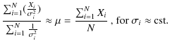
distributed according to a well-known distribution. However, the squared amplitude,
related to S2, should be distributed according to a
80% probability that the measurements are drawn from a normally -distributed
sample), the amplitudes of variability, being directly related to S, cannot be
distributed according to a well-known distribution. However, the squared amplitude,
related to S2, should be distributed according to a ![]() distribution with N-1 degrees
of freedom, which asymptotically approaches a normal distribution for large N (N being
typically 122 in our sample).
distribution with N-1 degrees
of freedom, which asymptotically approaches a normal distribution for large N (N being
typically 122 in our sample).
|
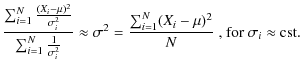
Figure 3:
Comparison
between the distribution in bins of magnitude and the
simulated results for the whole sample of OB stars superimposed in black
with the 3 intrinsic categories from Sect. 5. Bins are for Hp=[5, 5.5] ( left),
and Hp [9, 9.25] ( right). From top to bottom, the filled histograms
represent the number of OBMS, OBe and OBSG stars in the above-mentioned magnitude bins.
Note that there are a few points with a squared-amplitude that is off-scale in these diagrams;
these have not been shown for reasons of clarity. The solid line represents |
| Open with DEXTER | |
![\begin{figure}
\par\includegraphics[width=12cm,clip]{12304fg9.ps}
\end{figure}](/articles/aa/full_html/2009/44/aa12304-09/img37.png)
|
Figure 4:
Variability threshold calculated for our sample. |
| Open with DEXTER | |
To be more exact, we simulated bins with 10 000 stars (the actual number of stars in each
magnitude bin is actually closer to 100, but we chose 10 000 for greater reliability),
with 100 transits each and compared the outcome to the actual distribution of the squared
amplitude (
![]() )
in each magnitude bin. Magnitudes for a constant star
should be distributed according to a Gaussian centered on the mean magnitude, so the
simulation represents what the distribution inside a given bin of magnitude should look
like, if all the stars were constant. This is exactly what we are looking for, since
variable stars should be located outside this simulated squared-amplitude
distribution. We then adjusted the simulated squared-amplitude distribution to the real
distribution and placed the variability limit (
)
in each magnitude bin. Magnitudes for a constant star
should be distributed according to a Gaussian centered on the mean magnitude, so the
simulation represents what the distribution inside a given bin of magnitude should look
like, if all the stars were constant. This is exactly what we are looking for, since
variable stars should be located outside this simulated squared-amplitude
distribution. We then adjusted the simulated squared-amplitude distribution to the real
distribution and placed the variability limit (![]() ,
m for middle) at the point
where the simulated distribution reaches 0.1% of the maximum. The error on this limit is
represented by the
,
m for middle) at the point
where the simulated distribution reaches 0.1% of the maximum. The error on this limit is
represented by the
![]() (
(![]() Gaussian because
Gaussian because
![]() )
of the adjusted simulated distribution. The errors on the calculated
)
of the adjusted simulated distribution. The errors on the calculated
![]() are transformed to
are transformed to ![]() and
and ![]() with
with
![]() .
Sample-simulated and real distributions of the
squared-amplitude are represented in Fig. 3, where the distributions for the 3 different classes of intrinsic variability presented in Sect. 5 have been
overplotted. The error err on
.
Sample-simulated and real distributions of the
squared-amplitude are represented in Fig. 3, where the distributions for the 3 different classes of intrinsic variability presented in Sect. 5 have been
overplotted. The error err on ![]() is then transformed into the error on
is then transformed into the error on ![]() (
(
![]() )
to be representable in a more classical way in Fig. 4.
Note that err becomes err- and err+ in the
)
to be representable in a more classical way in Fig. 4.
Note that err becomes err- and err+ in the
![]() domain, i.e. the error
is asymmetrical.
domain, i.e. the error
is asymmetrical.
A fourth order polynomial is adjusted to the points in each bin of magnitude to
obtain the resulting thresholds presented in Fig. 4, where the 3 lines
represent the threshold ![]() minus the error to the lower side (
minus the error to the lower side (![]() ,
lower dash-dotted line), the threshold
,
lower dash-dotted line), the threshold ![]() itself (solid line) and
itself (solid line) and ![]() plus
the error to the higher side (
plus
the error to the higher side (![]() ,
upper dash-dotted line). We chose
,
upper dash-dotted line). We chose ![]() as
a conservative measure of the variability threshold, i.e. the 751 stars above
as
a conservative measure of the variability threshold, i.e. the 751 stars above
![]() are assumed to be variable. Between
are assumed to be variable. Between ![]() and
and ![]() lie ``possibly
variable stars'', while supposedly ``non variable'' stars are located below
lie ``possibly
variable stars'', while supposedly ``non variable'' stars are located below ![]() .
Table 1 presents the results in a general manner. As one can see, there is
a negligible fraction (<0.5%) of known periodic or variable stars below the
established lower limit (
.
Table 1 presents the results in a general manner. As one can see, there is
a negligible fraction (<0.5%) of known periodic or variable stars below the
established lower limit (![]() ). Moreover, no stars deemed as constant by the
HIPPARCOS consortium appear above the highest threshold
). Moreover, no stars deemed as constant by the
HIPPARCOS consortium appear above the highest threshold ![]() ,
thus validating ``a
posteriori'' our calculations. Most of the ``M'' stars are located in the ``possibly
variable'' zone which is normal, considering the small amplitude of their variations.
``D'' stars are mostly classified as ``non-variable'', a result that is also
encouraging, i.e. the number of stars wrongly classified as variable is minimal. In
addition, less than 2% of the total number of stars which could not be classified
lie above the threshold
,
thus validating ``a
posteriori'' our calculations. Most of the ``M'' stars are located in the ``possibly
variable'' zone which is normal, considering the small amplitude of their variations.
``D'' stars are mostly classified as ``non-variable'', a result that is also
encouraging, i.e. the number of stars wrongly classified as variable is minimal. In
addition, less than 2% of the total number of stars which could not be classified
lie above the threshold ![]() .
.
We assume all stars above ![]() to be variable,
hence (per our choice of
to be variable,
hence (per our choice of ![]() )
the probability of having a non-variable star
among the candidates is less than 0.1% as confirmed by the statistics (cf. Table 1). The probability of finding a variable star (with amplitude Amp.
)
the probability of having a non-variable star
among the candidates is less than 0.1% as confirmed by the statistics (cf. Table 1). The probability of finding a variable star (with amplitude Amp. ![]() 0.03 mag) below
0.03 mag) below ![]() is
is ![]() 1%, as indicated by the quasi absence of ``U'' or
``P'' stars, while it is around 15% for stars with a relatively low amplitude
(Amp.
1%, as indicated by the quasi absence of ``U'' or
``P'' stars, while it is around 15% for stars with a relatively low amplitude
(Amp. ![]() 0.03 mag). On the other hand, when considering stars below
0.03 mag). On the other hand, when considering stars below ![]() ,
the probability of finding a variable star rises to
,
the probability of finding a variable star rises to ![]() 10% for Amp.
10% for Amp. ![]() 0.03mag and
0.03mag and ![]() 70% for Amp.
70% for Amp. ![]() 0.03 mag. That is the reason why stars
located in this particular region have been classified as ``possibly variable
stars''. It comprises more than 80% of the microvariable stars and about 15% of
the ``U'' and ``P'' stars (cf. Table 1). The error on the magnitude is
0.03 mag. That is the reason why stars
located in this particular region have been classified as ``possibly variable
stars''. It comprises more than 80% of the microvariable stars and about 15% of
the ``U'' and ``P'' stars (cf. Table 1). The error on the magnitude is ![]() 0.002 mag on average and depends on the number of points for each star and on the
variability level. Some shifts in magnitude in Fig. 4 could modify the
distribution around the threshold by a few percent (
0.002 mag on average and depends on the number of points for each star and on the
variability level. Some shifts in magnitude in Fig. 4 could modify the
distribution around the threshold by a few percent (![]() 5%), below the limiting
magnitude (
5%), below the limiting
magnitude (
![]() mag) and more above it, but this is within the error margins in
the statistics of Table 2, which are quite large.
mag) and more above it, but this is within the error margins in
the statistics of Table 2, which are quite large.
It is important to stress
that the ``S/I'' method from Duquennoy et al. (1991) also provides us with the means to
verify a posteriori the accuracy of the calculated threshold, i.e. the
distribution of stars above and below the threshold. Indeed, the introduction of a
variable
![]() (Duquennoy et al. 1991) allows us to
calculate a threshold (TS/I) which does not depend on the magnitude. Applying a
false probability detection of 0.1% for this threshold, we find that the
distribution of stars above and below TS/I is similar to the distribution
above and below
(Duquennoy et al. 1991) allows us to
calculate a threshold (TS/I) which does not depend on the magnitude. Applying a
false probability detection of 0.1% for this threshold, we find that the
distribution of stars above and below TS/I is similar to the distribution
above and below ![]() within less than 5%. Of course, this is not surprising
considering the fact that we established that the internal error I was correctly
estimated and thus the shape of the internal error seen in Fig. 2 is
the same (
within less than 5%. Of course, this is not surprising
considering the fact that we established that the internal error I was correctly
estimated and thus the shape of the internal error seen in Fig. 2 is
the same (![]() 3.289) as that of
3.289) as that of ![]() (cf. Figs. 2 and 4).
(cf. Figs. 2 and 4).
4 Analysis of the variability
The 751 stars selected as ``variable'' thanks to our determined threshold were then analyzed with the CLEAN algorithm (Scargle 1982; Roberts 1987) followed by a Phase Dispersion Minimization technique (Stellingwerf 1978, PDM). For the CLEAN program we used a gain of 0.2 and a maximum number of 250 iterations. We calculated a false alarm probability (fap) threshold for each star and kept the three biggest power peaks of the CLEAN spectrum, only if they were above a 99% fap threshold. We then used the PDM around each of those peaks to locate the position more precisely.
5 Results and discussion
![\begin{figure}
\par\includegraphics[angle=-90,width=13cm,clip]{12304fg10.ps}
\end{figure}](/articles/aa/full_html/2009/44/aa12304-09/img48.png)
|
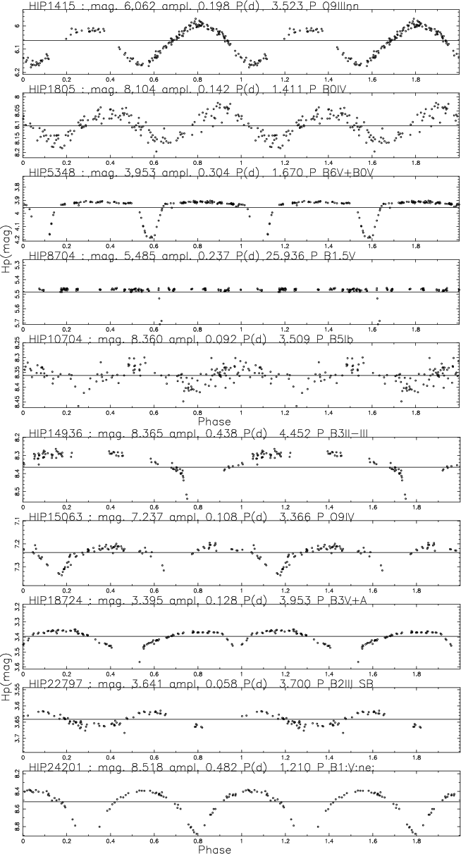
Figure 5:
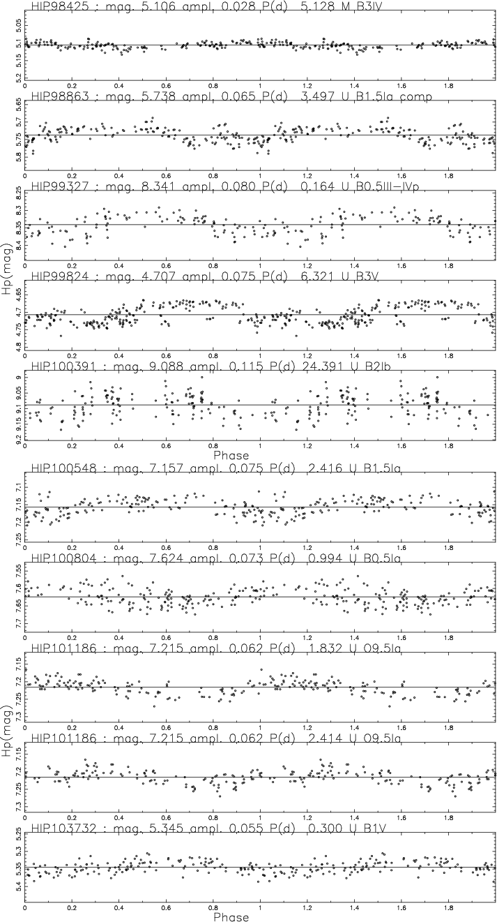
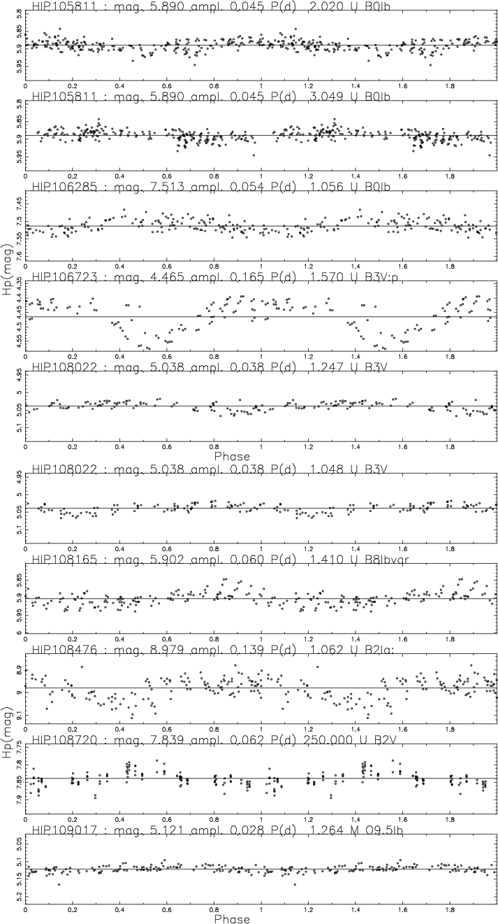
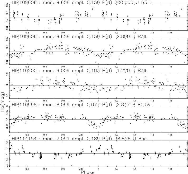
This figure is a representative extraction of our ``catalog of New
Periodic stars'' given in Appendix B2.
It plots Hp mag. vs. Phase. The epoch is arbitrarily taken as JD-2 440 000
=7800, which is the beginning of the HIPPARCOS observations. On top of each lightcurve are the HIPPARCOS
number, the Hp magnitude and mean amplitude calculated in this study, the period, variability flag and spectral
type from the HIPPARCOS data (periods can also be new ones). The Hp magnitude, mean amplitude and periods
are accurate to |
| Open with DEXTER | |
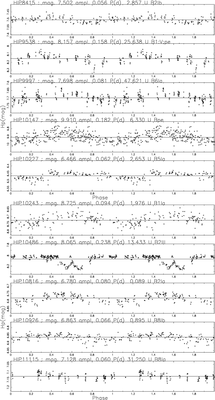
Of the 227 previously known periodically varying stars (flagged ``P''), about 90% were found to be periodic in this study, some with revised periods. The 10% discrepancy between HIPPARCOS and this study most probably comes from the difference in the number of points in the analysis. The HIPPARCOS consortium excluded all the flagged points while we kept some of them, hence the difference.
We chose to classify the supposedly variable stars in 4 broad categories. These include, first under intrinsic variables: OB stars of luminosity classes I and II (OBSG), Main sequence (III to V) stars with no emission (OBMS) and OB stars in luminosity classes III to V with emission (OBe stars) and then under extrinsic variables: eclipsing binaries (E). Some eclipsers may reveal other types of variability but the eclipse phenomenon usually dominates, so we will retain them only in the E category. As for types of variability, we follow the definition in the General catalog of Variable Stars (GCVS, Samus et al. 2004) and of Gautschy & Saio (1996). The principal variability types used are listed in Appendix A. Note that stars for which the lightcurve is not precise enough to decide between an ellipsoidal variable and an eclipsing binary, were given preference as eclipsing binaries.
We found 169 stars with new periods, of which ![]() 50% were also found by
Koen & Eyer (2002). Included in these new periodically varying stars, are 5 new
eclipsing binaries of which 1 was also in Koen & Eyer (2002) and 2 were found by
Otero (2003). The phase plots of stars with new periodicities are given in
Appendix B (see Fig. 5). When classifying the variability types, all of
the probable periods have been taken into account; we made no assumptions on the
veracity of those periods. However, periods of
50% were also found by
Koen & Eyer (2002). Included in these new periodically varying stars, are 5 new
eclipsing binaries of which 1 was also in Koen & Eyer (2002) and 2 were found by
Otero (2003). The phase plots of stars with new periodicities are given in
Appendix B (see Fig. 5). When classifying the variability types, all of
the probable periods have been taken into account; we made no assumptions on the
veracity of those periods. However, periods of
![]() d are probably
related to the orbital period of the HIPPARCOS satellite as discussed in
Koen & Eyer (2002), so they have not been taken into account when classifying the
types of variability. To indicate any ``unsure'' status of the new periods, we added
question marks to the variability types (Appendix A tables).
d are probably
related to the orbital period of the HIPPARCOS satellite as discussed in
Koen & Eyer (2002), so they have not been taken into account when classifying the
types of variability. To indicate any ``unsure'' status of the new periods, we added
question marks to the variability types (Appendix A tables).
Our complete sample of OB stars consists of 127 eclipsing (or supposed as eclipsing)
binaries, 229 OBe stars, 1482 OBMS stars and 577 OBSG stars. The statistics for all
the categories are presented in Tables 2 (intrinsic categories) and 3 (eclipsing binaries), while the details are presented in a separate
table in Appendix A. The errors on the proportions in Tables 2 and 3 are based on the assumption that the numbers of stars in a given
category (Ni compared to
![]() )
arise from a Binomial distribution (which
tends towards a Poisson distribution for
)
arise from a Binomial distribution (which
tends towards a Poisson distribution for
![]() ), hence
), hence
![]() ,
which gives an estimated error
margin with a confidence interval of 99% of
,
which gives an estimated error
margin with a confidence interval of 99% of
![]() ,
and an error in percent of
,
and an error in percent of
![]() ,
where
,
where
![]() is the proportion and
is the proportion and
![]() the number of stars
in the chosen sub-sample.
the number of stars
in the chosen sub-sample.
Moreover, we recalculated the proportions taking the 7 previously known periodically varying stars that were deleted because of too many flagged points and concluded that their influence is negligible, as can be seen from the row labeled ``Not included'' in Table 2. Note that the HIPPARCOS satellite scans along an axis with a ``scan-data angle'' depending on the time of observation. Thus, the more a source is extended, the more the variation of this angle can induce false variability. This angle is mainly sensitive to extended sources and nebulosities. This will be discussed in Sect. 5.2.
Table 2: OB Stars in the 3 OB categories and corresponding statistics.
Table 3: OB eclipsing Stars in the 3 OB categories and corresponding statistics.
One can see from Table 2 that OBe stars are much more variable
intrinsically than OBSG or OBMS stars, and also more variable than the complete
sample (line labeled ``OBi,v vs. tot. OBi''). On the other hand, OBMS stars are
below ![]() in 83% of cases, which means they are mostly non variable (53% are
classified as non-variable, against 11% for the OBe stars and 34% for the OBSG
stars). Figure 6 also shows these aspects in a different way. One can
see in that figure that OBe stars are over-represented above the threshold
in 83% of cases, which means they are mostly non variable (53% are
classified as non-variable, against 11% for the OBe stars and 34% for the OBSG
stars). Figure 6 also shows these aspects in a different way. One can
see in that figure that OBe stars are over-represented above the threshold ![]() .
This will be developed in Sects. 5.1 and 5.2.
.
This will be developed in Sects. 5.1 and 5.2.
|
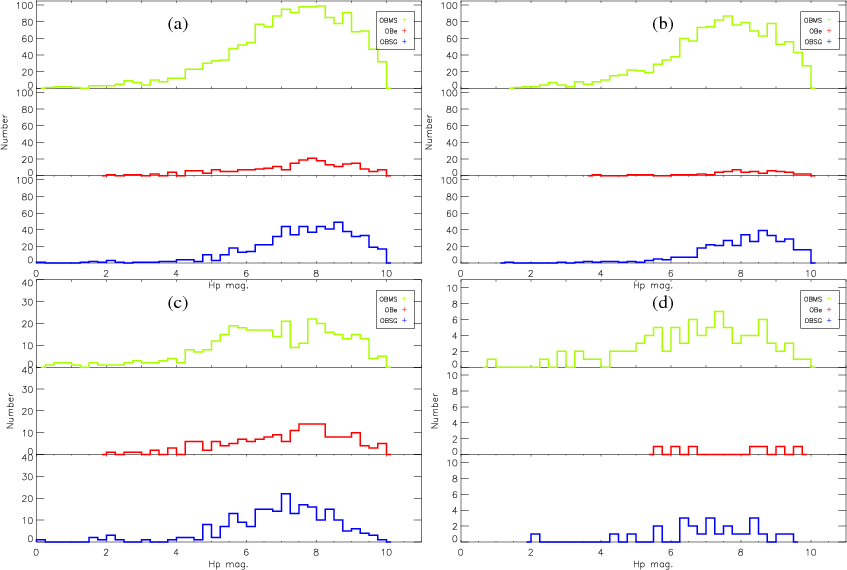
Figure 6:
The four panels of this figure represent the distribution in magnitude for
the 3 intrinsic variability classes in 4 different situations. From top to bottom, OBMS stars, OBe stars and OBSG stars. a) The whole
sample of 2407 stars, b) the 1656 stars below |
| Open with DEXTER | |
5.1 Extrinsic variability: eclipsing binaries
All the eclipsing binary lightcurves are presented in Appendix B, an extraction of which is presented here in Fig. 7. They are also summarized, along with their variability types, in Appendix A, of which Table 4 is the beginning. When taking into account only the stars down to Hp=8, the statistics from Table 3 do not vary significantly (i.e., the proportions are identical).
![\begin{figure}
\par\includegraphics[angle=-90,width=15cm,clip]{12304fg15.ps}
\end{figure}](/articles/aa/full_html/2009/44/aa12304-09/img109.png)
|
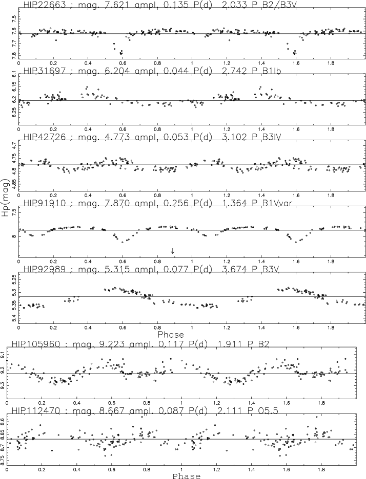
Figure 7:
This figure is the beginning of our ``catalog of Eclipsing Binaries''
given in Appendix B1. It contains 122 candidates; the remaining 5 are in
Appendix B3 and B4.
It plots Hp mag. vs. Phase. The epoch is arbitrarily taken as JD-2 440 000
=7800, which is the beginning of the HIPPARCOS observations. On top of each lightcurve are the HIPPARCOS
number, the Hp magnitude and mean amplitude calculated in this study, the period, variability flag and
spectral type from the
HIPPARCOS data (periods can also be new ones). The Hp magnitude, mean amplitude and periods
are accurate to |
| Open with DEXTER | |
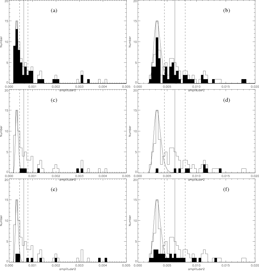
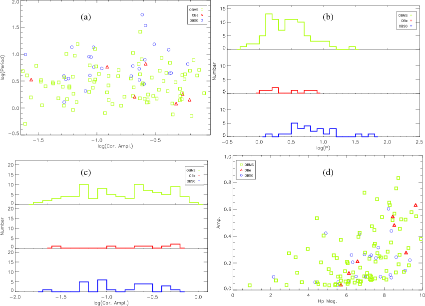
Figure 8 presents the periods and amplitudes of variation for the eclipsing binaries in the 3 classes of intrinsic variability. The amplitude of Fig. 8 is representative of the depths of the eclipses, but not as precisely as for other types of variability. Indeed, the estimation of the peak-to-peak amplitude works better the more the lightcurve approaches a sinusoid. In the case of a detached system, where the primary and the secondary minima are very different, the accuracy of the estimation of the amplitude strongly depends on the number of points during the eclipses versus those between.
|
Figure 8: Eclipsing binaries: the upper left panel a) presents the log of the period (days) versus the log of the amplitude of the variations, while the upper right panel b) presents the histograms of the periods in the 3 intrinsic variability classes OBMS, OBe and OBSG. Squares represent OBMS stars, triangles OBe stars and circles OBSG stars. The lower left panel c) presents the histograms of the amplitude in the 3 intrinsic variability classes. The lower right panel d) presents the amplitude vs. Hp magnitude. |
| Open with DEXTER | |
Table 4 also shows that there are twice as many contact (EB) systems
as detached (EA) among the OBMS stars, while there are about as many contact as
detached systems among OBSG stars. This will be discussed in Sect. 5.2
in their respective categories although this is not an intrinsic variability. Note the
difference in the peaks of the period histograms between the OBSG and the OBMS
stars. The orbital periods seem to be larger for OBSG stars on average. This
difference is highly significant (![]() )
according to the Wilcoxson criterion (Wilcoxon 1945).
It is also seen when considering the sample to the limit of completeness (i.e. below Hp=8 mag).
)
according to the Wilcoxson criterion (Wilcoxon 1945).
It is also seen when considering the sample to the limit of completeness (i.e. below Hp=8 mag).
Table 4: OB eclipsing binaries of the HIPPARCOS catalog.
5.2 Intrinsic variability
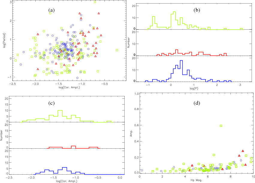
Figure 9 presents the periods and amplitudes of variation in the 3 classes of intrinsic variability. Periods in the 3 classes appear equally distributed in this figure, although if we consider only the periods already found by HIPPARCOS (allowing for the fact that our periods might not be reliable) the peak from the OBSG class seems to occur at a slightly longer period than the OBMS-class peak (8d compared to 3d). This could be easily explained by the well-known period-mass relation: the greater the mass of the star, the larger its radius, the lower its mean density, and therefore the longer its pulsation period. This relation should basically apply to all the OB stars studied here. Moreover, there seems to be a gap in Fig. 9a and b between P=0.3d and P=1d, whose origin remains unknown.
|
Figure 9:
Variable stars: from top to bottom, left to right. Colors and symbols are the same as in
Fig. 8. The first panel a) presents the
log of the period (days) versus the amplitude of the variations, while the second panel b) presents
the histograms of the periods in the 3 intrinsic variability classes
of OBMS, OBe and OBSG stars ( from bottom to top). The third panel c) presents the amplitude histograms
of the same 3 classes of variability, and the fourth d) is the same as Fig. 4
for the periodic stars above |
| Open with DEXTER | |
Note that the first and second panels of Fig. 9 take the new periods into
account, while the third and fourth do not. This is because some of the stars have several
periods which are associated with identical amplitudes and magnitudes. The total numbers
of stars are 56, 7 and 29 for the OBMS, OBe and OBSG categories, respectively, in the
amplitude histogram (lower left panel), while they reach 108, 39 and 121 in the period
histogram (upper right panel), because they include all the possible new periods. It is
interesting in this case to note that the total number of OBe periods is more than five
times higher if we add the new periods (number of
![]() ). On the other hand, the
total number of OBSG periods (including new periods) is about 4 times the initial number
of OBSG periods, while the number of new periods found in the OBMS stars class is modest
(
). On the other hand, the
total number of OBSG periods (including new periods) is about 4 times the initial number
of OBSG periods, while the number of new periods found in the OBMS stars class is modest
(
![]() ).
).
5.2.1 OB Main Sequence stars
Not surprisingly, OBMS stars represent the greater part of our OB sample of stars
(65%). Their variability classification is presented in Table 5. As
can be seen in Table 2, less than 20% of them are classified as variable
in this study, which is rather low compared to the percentage of variable OBe and
OBSG stars (OBe: 75%, OBSG: 35%). In fact, about 30% of all the stars in the
sample are supposedly variable, and the proportion of variable OBMS stars is below
that average. This is easily explained when one considers the fact that main
sequence stars are much more stable than the two other categories involved here.
There also seem to be more eclipsing systems among this class (cf. Table 3). It is not impossible that this is due to the fact that the stability
of these stars prevents them from merging as often as the stars in the other
categories, hence the higher number of non-merged eclipsing binaries
(Podsiadlowski 2006). Moreover, despite the limited sample, there is a trend
towards more EB (contact) systems than EA (detached). Indeed there are
![]() 60% EB eclipsing binaries compared to
60% EB eclipsing binaries compared to ![]() 30% EA eclipsing binaries
(the rest are classified as E or EW). The statistics stay the same if we consider
only the stars with
30% EA eclipsing binaries
(the rest are classified as E or EW). The statistics stay the same if we consider
only the stars with
![]() mag. This might be related to the fact that OBMS
stars in binary systems are closer together than the stars in our other categories, and thus
easier to detect (i.e., the inclination angle can deviate more from 90
mag. This might be related to the fact that OBMS
stars in binary systems are closer together than the stars in our other categories, and thus
easier to detect (i.e., the inclination angle can deviate more from 90![]() ,
because the components are closer).
,
because the components are closer).
5.2.2 OBe stars
Table 5:
OBMS stars above the threshold ![]() .
.
The variability classification of OBe stars is presented in Table 6. We mention that the OBe stars we defined here are in fact Oe and Be stars. Oe stars were first introduced by Conti & Leep (1974), and usually fall inside the range O9-B0. However, Negueruela et al. (2004) mention that some published spectral types are too early most likely due to filling in of HeI lines. That is why we also included spectral types earlier than O9. Although Oe stars do not show the presence of a disk as in Be stars they are considered to be the extension of the Be stars to the O type stars.
As noted earlier, OBe stars seem to be by far the most variable class
in our 3
intrinsic categories. Indeed the incidence of rapid rotation and
pulsations and their possible interactions could explain this high
level
of variability. These hypotheses are strengthened by the apparent
correlation found between pulsations and
an outburst in the COROT observations of the B0e star HD 49330 (Huat 2009).
Moreover, OBe stars are nearly absent below the threshold ![]() and the cause may be that even if the variability is not periodic,
a few outbursts might have been picked up by HIPPARCOS observations and lead to high amplitude variability. As
for the variability of the ``scan-data angle'' noted earlier,
Quirrenbach et al. (1997) note that the disks, if present, have negligible (for the
HIPPARCOS satellite optics) extensions in the optical of a few milli-arcseconds. So
this cannot account for variations seen in OBe stars. It does not apply, though, to
any flux variations due to the instabilities in the disks which can augment the
variability of the star.
and the cause may be that even if the variability is not periodic,
a few outbursts might have been picked up by HIPPARCOS observations and lead to high amplitude variability. As
for the variability of the ``scan-data angle'' noted earlier,
Quirrenbach et al. (1997) note that the disks, if present, have negligible (for the
HIPPARCOS satellite optics) extensions in the optical of a few milli-arcseconds. So
this cannot account for variations seen in OBe stars. It does not apply, though, to
any flux variations due to the instabilities in the disks which can augment the
variability of the star.
In addition, a good fraction (20-60%) of OBe stars are supposed to be in a post mass-transfer phase of a close binary system (Pols et al. 1991). The upper right panel of Figure 8 seems to indicate that OBe star periods do not reach as high as OBMS star periods. However, when taking into account the actual numbers with a Wilcoxon test (7-OBe against 89-OBMS EB Periods), the difference between both distributions is significant only to a level of 60% (Wilcoxon 1945; Mann & Whitney 1947). It would be of considerable interest to see if this tendency is confirmed in a larger sample of OBe binary systems.
5.2.3 OB supergiants stars
Table 6:
OBe stars above the threshold ![]() .
.
Table 7:
OBSG stars above the threshold ![]() .
.
OB supergiants are usually thought to be more prone to variability, mainly because
of their large radii, thus weaker surface gravity, and subsequent tendency to be
unstable. When we take the total sample of stars, we find that about 30% of the
variable stars (above ![]() )
are OBSGs, while only about 20% of the non-variables
(below
)
are OBSGs, while only about 20% of the non-variables
(below ![]() )
are OBSGs. A finer analysis with different bins in magnitude
confirms this tendency. Below Hp=8 mag, OBSG stars are about twice as often above
)
are OBSGs. A finer analysis with different bins in magnitude
confirms this tendency. Below Hp=8 mag, OBSG stars are about twice as often above
![]() than below (Hp<6: 11% below
than below (Hp<6: 11% below ![]() ,
,
![]() 23% above
23% above ![]() ;
6 <
Hp < 8, <18% below
;
6 <
Hp < 8, <18% below ![]() ,
,
![]() 32% above
32% above ![]() ). This would tend to
indicate that OBSG stars are globally more variable than OB stars in general.
Fainter than Hp=8 mag, on the other hand, there is no real difference between the
percentage of OBSGs above and below
). This would tend to
indicate that OBSG stars are globally more variable than OB stars in general.
Fainter than Hp=8 mag, on the other hand, there is no real difference between the
percentage of OBSGs above and below ![]() (OBSGs
(OBSGs ![]() 25% of OB above and
below
25% of OB above and
below ![]() ,
cf. Table 8) but this is probably due to the incompleteness
of the sample, thus the increased scatter of the instrumental error fainter than Hp=8 mag.
,
cf. Table 8) but this is probably due to the incompleteness
of the sample, thus the increased scatter of the instrumental error fainter than Hp=8 mag.
![\begin{figure}
\par\includegraphics[width=8.8cm,clip]{12304fg24.ps}
\end{figure}](/articles/aa/full_html/2009/44/aa12304-09/img119.png)
|
Figure 10: Periodicities as a function of spectral type and luminosity class (cf. de Jager 1980). The tracks have been plotted according to the values of Vanbeveren et al. (1998). Symbol size is proportional to the amplitude of the variation. |
| Open with DEXTER | |
We also studied the distribution of periods in OBSGs to see if the trends seen in
de Jager (1980, p.343) appear with our much larger sample of OBSG stars. As
can be seen in Fig. 10, there is a tendency for longer periods
(
![]() )
to be located near the upper right corner of the diagram, while
shorter periods (
)
to be located near the upper right corner of the diagram, while
shorter periods (
![]() )
are located nearer to the lower left corner of the
diagram. Intermediate periods (
)
are located nearer to the lower left corner of the
diagram. Intermediate periods (
![]() )
are mostly located between the above two
groups. Short periods (
)
are mostly located between the above two
groups. Short periods (
![]() )
are more scattered across the diagram (although still
more to the lower left), but this tendency also appears when the new periods (some
of them are not reliable) are not taken into account. Longer periods (
)
are more scattered across the diagram (although still
more to the lower left), but this tendency also appears when the new periods (some
of them are not reliable) are not taken into account. Longer periods (
![]() )
are
too few to conclude anything. Nevertheless, we confirm the effect shown in
de Jager (1980) for a bigger sample with greater spread in spectral
types. All the ``variable'' OBSG stars and their parameters are presented in Table 7.
)
are
too few to conclude anything. Nevertheless, we confirm the effect shown in
de Jager (1980) for a bigger sample with greater spread in spectral
types. All the ``variable'' OBSG stars and their parameters are presented in Table 7.
Figure 8 also shows that there is a tendency for OBSG systems to have longer periods. This might be attributed in part to the larger size of the components (Söderhjelm & Dischler 2005).
Finally, we note that the number of detached (EA) versus contact (EB) binary systems in this category is about equal, compared to a higher fraction of contact binaries among OBMS stars. Considering that surviving supergiant systems would have to have been farther apart than those that merged (Podsiadlowski 2006), this explains a greater relative number of detached systems among OBSGs.
Table 8: OBSG star proportions in 3 mag bins.
5.3 Special cases
Table 9:
Periodic stars not included
because of too many flagged points or below ![]() .
.
All the previously known periodically varying stars that were deleted because of a
significant number of flagged points or were located below ![]() ,
are presented in
Table 9 and their lightcurves are presented in Appendix B3 and B4. As
indicated by their number (
,
are presented in
Table 9 and their lightcurves are presented in Appendix B3 and B4. As
indicated by their number (![]() 1%), their effect on the threshold
calculations is negligible. Moreover, the distribution of their periodicities and
amplitudes does not visibly differ from the above results, and the 4 periodic OBSG
stars that were deleted or located below the threshold
1%), their effect on the threshold
calculations is negligible. Moreover, the distribution of their periodicities and
amplitudes does not visibly differ from the above results, and the 4 periodic OBSG
stars that were deleted or located below the threshold ![]() have periods in the
range P<5 days and would not influence the interpretation of Fig. 10.
have periods in the
range P<5 days and would not influence the interpretation of Fig. 10.
As mentioned earlier, LBV stars HR Car, AG Car and P Cyg (B2evar, B2:pe and B2pe, respectively) have been included in the OBe category. They represent 1% of the OBe stars and considering the error of 4% (cf. Table 2) on the level of variability of this class, it is not significant. Moreover, their HIPPARCOS data do not show any periodic variations and thus do not influence the results of the analysis of the periodic components. There are also a few unconfirmed LBV candidates according to Clark et al. (2005) within our sample but we cannot exclude them from this analysis without further evidence of their true status.
Star HIP34646 (HD55173, B3/5V(p)) was flagged under category 2 (corresponding to FAST data only) part of the time, hence the origin of the scatter. The unflagged points correspond to the ``seemingly perfect'' eclipsing binary lightcurve. However the value of the peak-to-peak amplitude indicated in the table in Appendix A represents the real amplitude of the variations due to binarity because the errors (significantly larger on the flagged points in this case) were taken into account.
Stars HIP65474 and HIP81305 have been classified as binaries (with ``?'') because of the shape of the dips seen in the lightcurves and the position of the lack of points about 0.5 phase later than the ``first'' dip. Of course, our choice can be discussed as stressed by ``?'' added to their variability type, but in this case, those two stars do not affect the statistics.
Star HIP10486 is definitely variable, almost certainly periodic but we do not have the definitive period. It might be an eclipsing binary but changing the period might affect the shape of our light curve to a large extent. Stars HIP31593 and HIP78526 belong to the eclipsing binary group as shown in Table 4. They have also been represented in the ``New periodic variables'' group because they were not detected as variable before this study (HIP31593) or before the article by Otero et al. (2003, HIP78526).
Some Be stars show typical outbursts (e.g. HIP32947, HIP35933, HIP74147, HIP88149). There are 3 studied Oe stars in the sample (HIP27941, HIP37074 and HIP30722) and their spectral types have been estimated to be too early (Negueruela et al. 2004), they are rather O8.5Ve, B0IVe and O9.5IVe, respectively. Rauw et al. (2007) find long term spectroscopic variations for HIP30722 (HD45314) and HIP37074 (HD60848), and our study points toward a new shorter period of 2.983 days for HIP37074, that remains to be studied in more detail.
6 Conclusions
First of all, we note that although this analysis is presented for ![]() mag,
the sample is complete only down to Hp=8 mag. All the figures and statistics have
also been calculated when limiting the sample to Hp=8 mag, and no major difference
was noted. Thus the conclusions are not affected by our choice of limiting
magnitude.
mag,
the sample is complete only down to Hp=8 mag. All the figures and statistics have
also been calculated when limiting the sample to Hp=8 mag, and no major difference
was noted. Thus the conclusions are not affected by our choice of limiting
magnitude.
In our sample, there are about ![]() % intrinsically variable stars, which
compares to the statistics given in Marchenko et al. (1998) for the WR-stars of
% intrinsically variable stars, which
compares to the statistics given in Marchenko et al. (1998) for the WR-stars of
![]()
![]() %. These results are similar, with a possibly higher variability
among WR stars probably induced by the presence of the dense stellar winds (e.g.,
rotational modulation: WR6, dust formation episodes or blobs: WR137).
%. These results are similar, with a possibly higher variability
among WR stars probably induced by the presence of the dense stellar winds (e.g.,
rotational modulation: WR6, dust formation episodes or blobs: WR137).
This analysis has enabled us to constrain the differences of variability among three classes of intrinsic variability (OBMS, OBe and OBSG stars). Indeed, OBe stars are much more variable than the two other intrinsic classes (75% compared to 17 and 35% for OBMS ans OBSG stars, respectively). The large physical sizes of the OBSG stars may explain the longer periods, compared to the OBMS sample, of the eclipsing binaries with an OBSG component. On the other hand, we note that there are more eclipsing binaries among OBMS stars, probably because those stars are more stable. Moreover, the proportion of contact systems is twice that of detached systems among OBMS stars. This might be an observational bias related to the closeness of the components in OBMS systems (i.e., contact systems are more variable and thus easier to observe).
The unique photometric data base of the HIPPARCOS program archive has enabled us to find a number of useful trends in variability among OB stars. It is expected that large, uniform photometric programs, space or ground-based, will provide even more impressive quantities of data of even higher quality. It is already the case for space missions such as the Canadian satellite MOST, the European COROT and the newly launched KEPLER mission. Large quantities of extremely precise data will soon enable one to enlarge this kind of statistical analysis of the variability of OB stars on other timescales.
AcknowledgementsWe would like to thank the referee for very useful comments on this work. LL's work is supported by the CNES. A.F.J.M. is grateful for financial support from NSERC (Canada) and FQRNT (Québec).
References
- Clark, J. S., Larionov, V. M., & Arkharov, A. 2005, A&A, 435, 239 [EDP Sciences] [CrossRef] [NASA ADS]
- Conti, P. S., & Leep, E. M. 1974, ApJ, 193, 113 [CrossRef] [NASA ADS]
- de Jager, C. 1980, Geophys. Astrophys. Monographs, 19
- Duquennoy, A., Mayor, M., & Halbwachs, J.-L. 1991, A&AS, 88, 281 [NASA ADS]
- ESA 1997, VizieR Online Data Catalog, 1
- Gautschy, A., & Saio, H. 1996, ARA&A, 34, 551 [CrossRef] [NASA ADS]
- Huat, A.-L. 2009, A&A, 0, 0
- Koen, C., & Eyer, L. 2002, MNRAS, 331, 45 [CrossRef] [NASA ADS]
- Mann, H., & Whitney, D. 1947, Annals Math. Stat., 18, 50 [CrossRef]
- Marchenko, S. V., Moffat, A. F. J., van der Hucht, K. A., et al. 1998, A&A, 331, 1022 [NASA ADS]
- Negueruela, I., Steele, I. A., & Bernabeu, G. 2004, Astron. Nachr., 325, 749 [CrossRef] [NASA ADS]
- Otero, S. A. 2003, Informational Bulletin on Variable Stars, 5480, 1
- Podsiadlowski, P. 2006, in Sacacomie Workshop: Massive Stars in Interacting Binaries
- Pols, O. R., Cote, J., Waters, L. B. F. M., & Heise, J. 1991, A&A, 241, 419 [NASA ADS]
- Quirrenbach, A., Bjorkman, K. S., Bjorkman, J. E., et al. 1997, ApJ, 479, 477 [CrossRef] [NASA ADS]
- Rauw, G., Naze, Y., Marique, P. X., et al. 2007, Information Bulletin on Variable Stars, 5773, 1
- Samus, N. N., Durlevich, O. V., et al. 2004, VizieR Online Data Catalog, 2250, 0
- Söderhjelm, S., & Dischler, J. 2005, A&A, 442, 1003 [EDP Sciences] [CrossRef] [NASA ADS]
- Vanbeveren, D., van Rensbergen, W., & de Loore, C. 1998, The brightest binaries, ed. D. Vanbeveren, W. van Rensbergen, & C. De Loore (Boston: Kluwer Academic), Ap&SS library, 232
- Walborn, N. R., & Fitzpatrick, E. L. 1990, PASP, 102, 379 [CrossRef] [NASA ADS]
- Wilcoxon, F. 1945, Biometrics Bull., 1, 80 [CrossRef]
Appendix A: Variable OB stars in the HIPPARCOS catalog according to this study
This appendix presents tables of the stars classified as ``variable'' in this study. The variability types used here are described in the ``general catalog of variable stars'' (Samus et al. 2004) and in Gautschy & Saio (1996). The main types are I, IA, L, SDOR et GCAS for irregular variations; ACYG, BCEP, SPB, ACV, PVTEL, SR, SXARI for pulsating stars; and E, EA, EB for eclipsing binaries.Table A.1: OB eclipsing binaries of the HIPPARCOS catalog.
Table A.2:
OBMS stars above the threshold ![]() .
.
Table A.3:
OBe stars above the threshold ![]() .
.
Table A.4:
OBSG stars above the threshold ![]() .
.
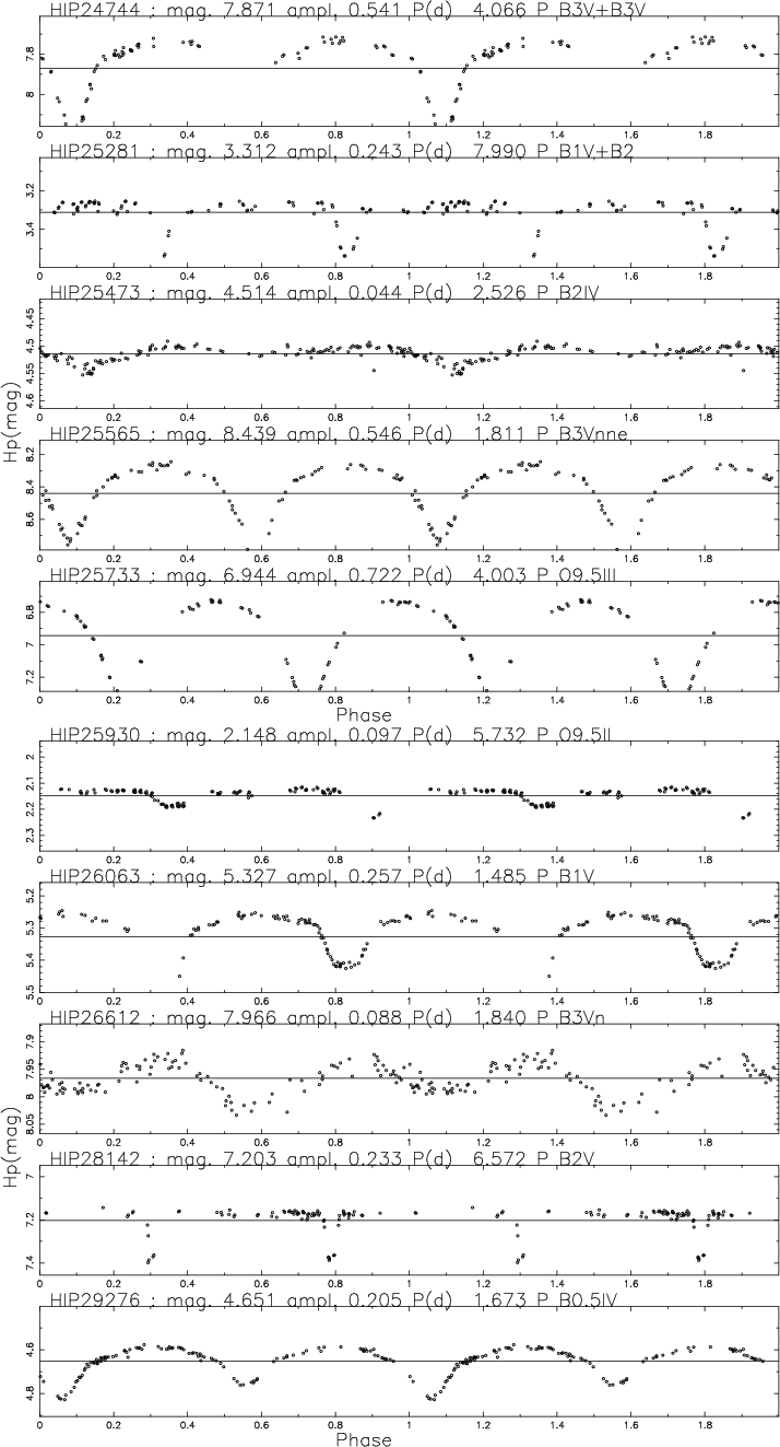
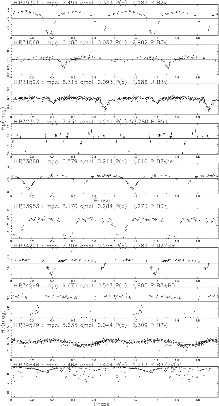
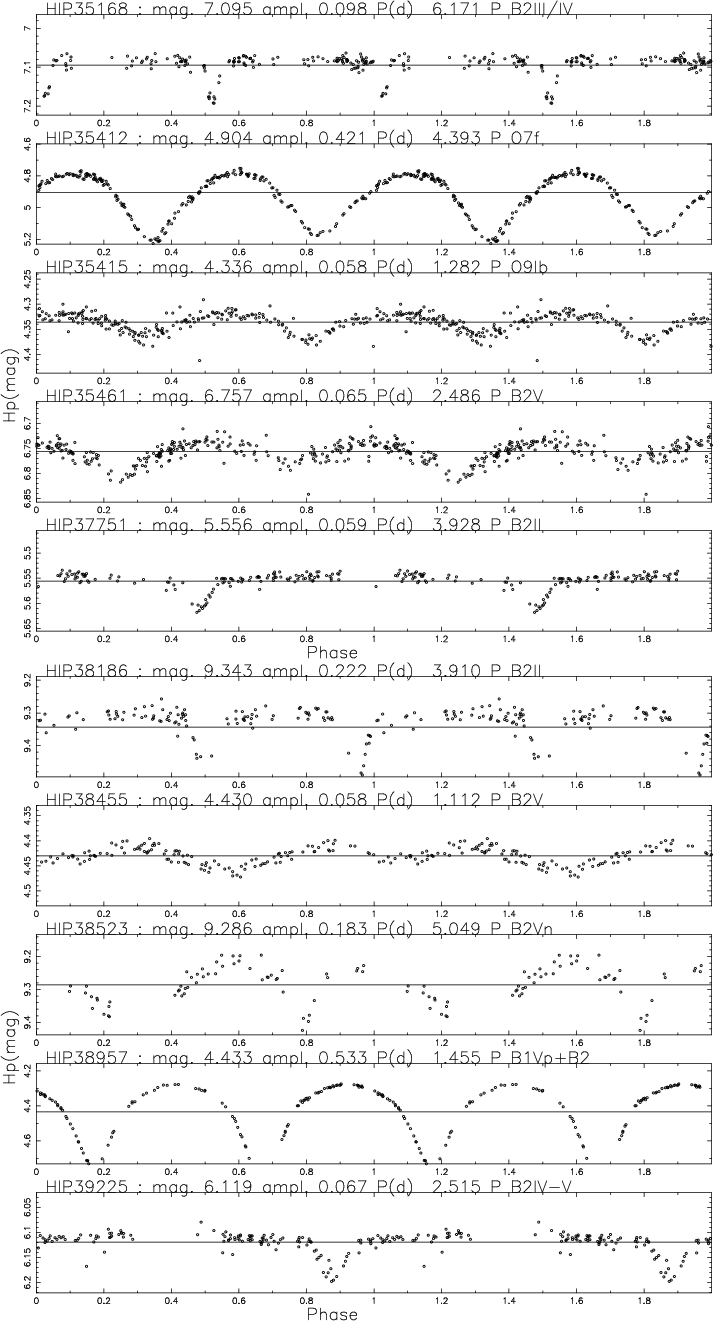
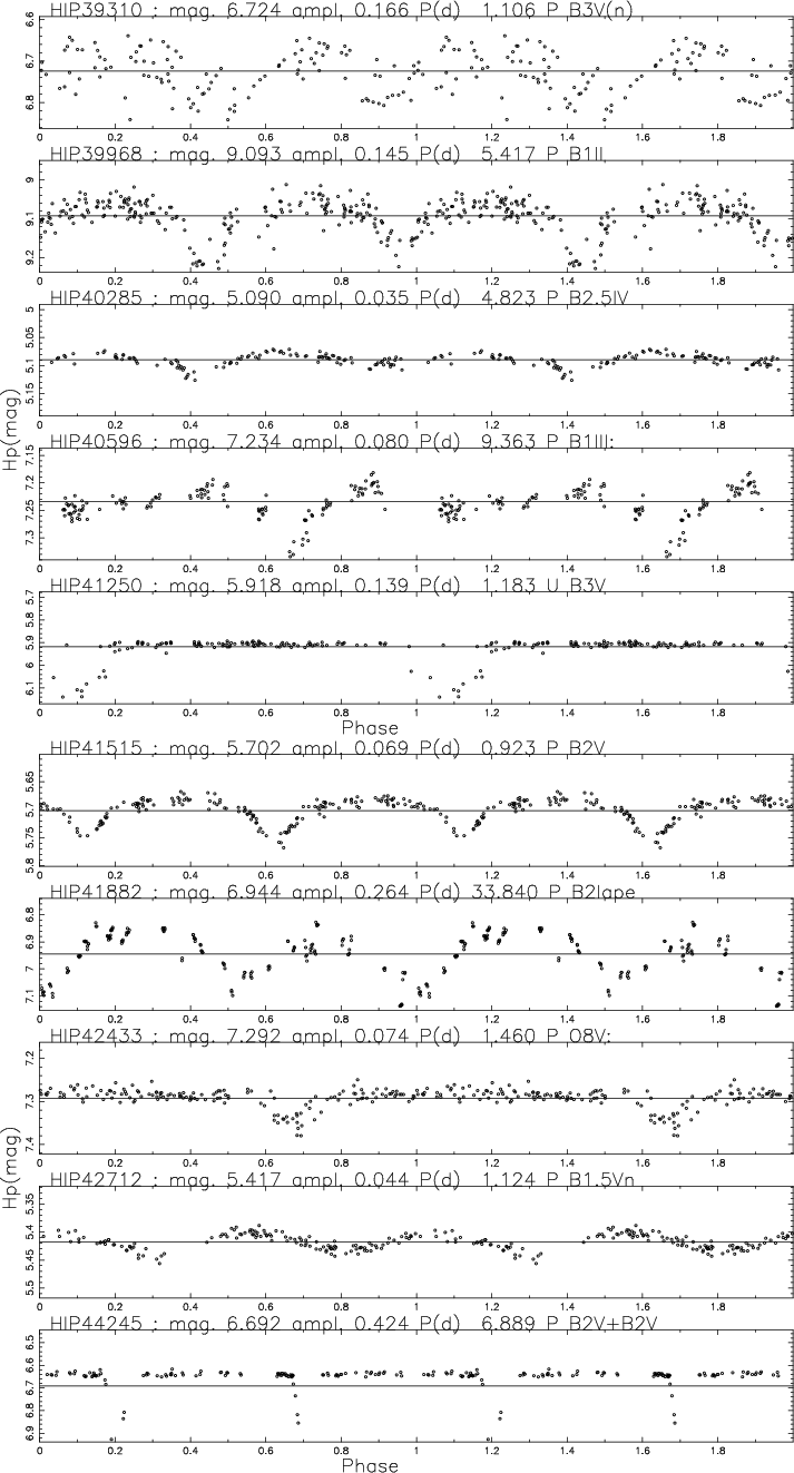
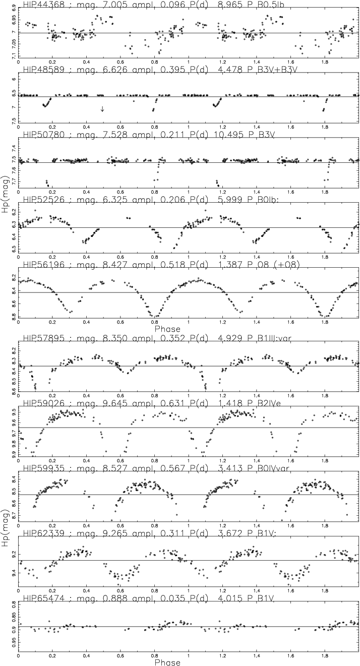
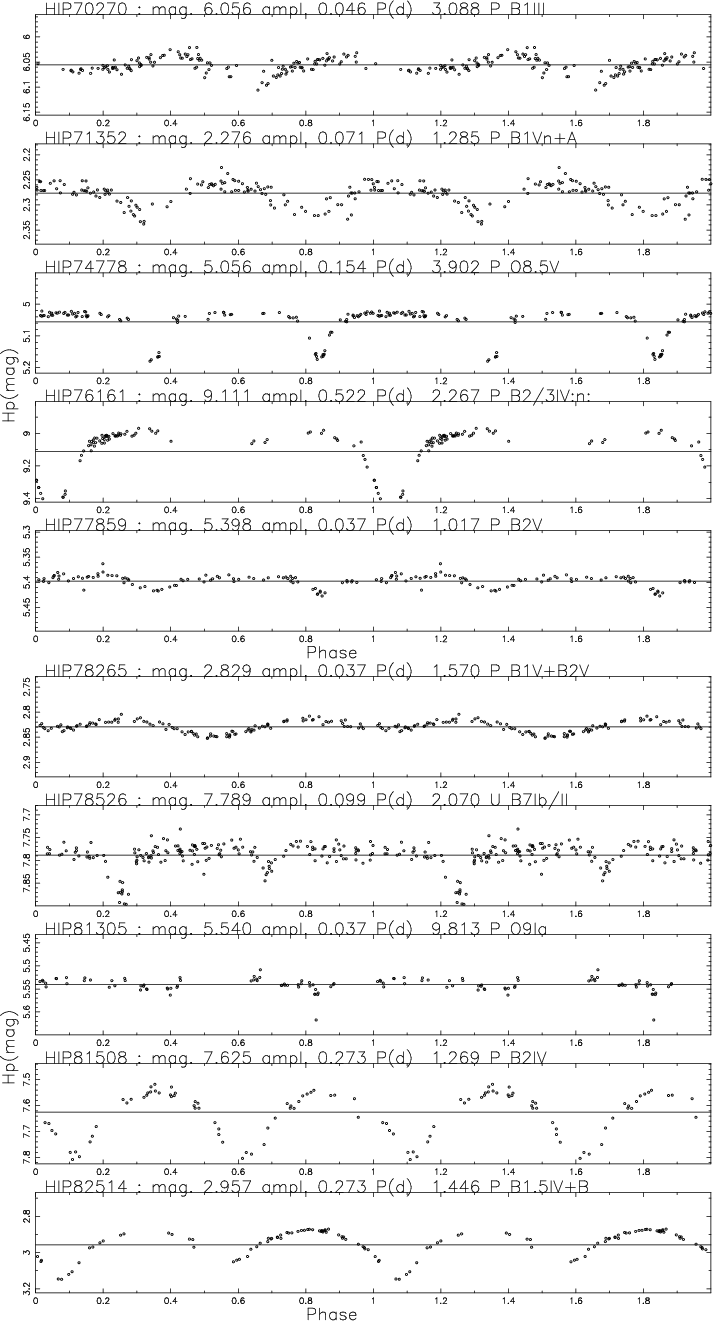
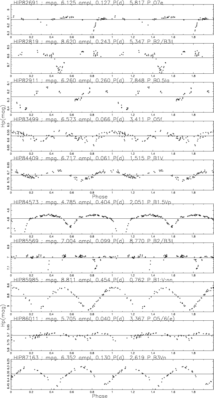
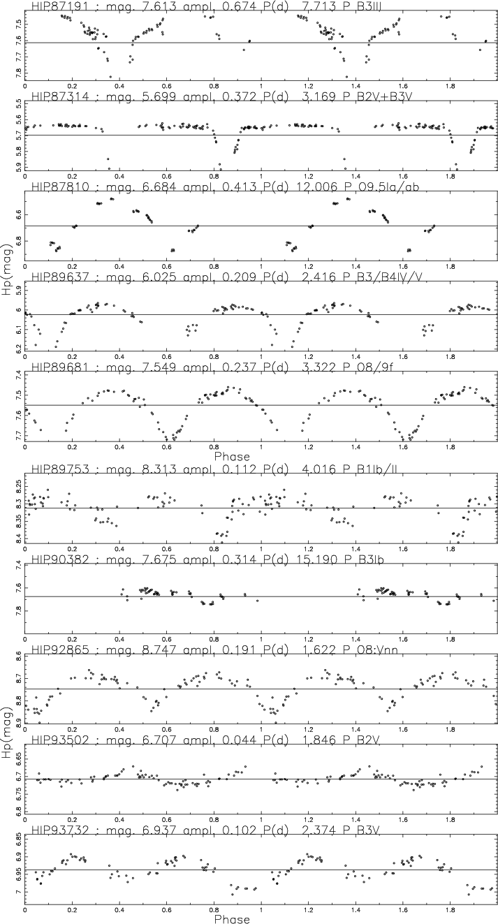
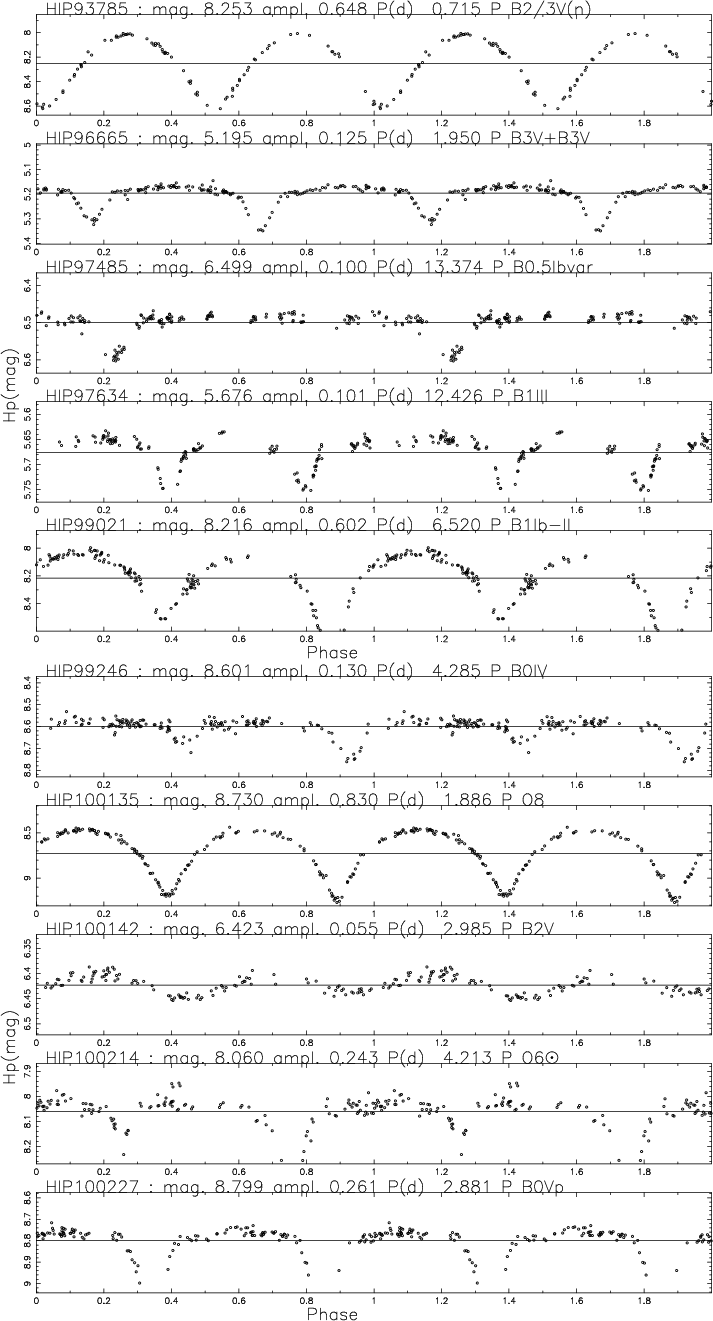
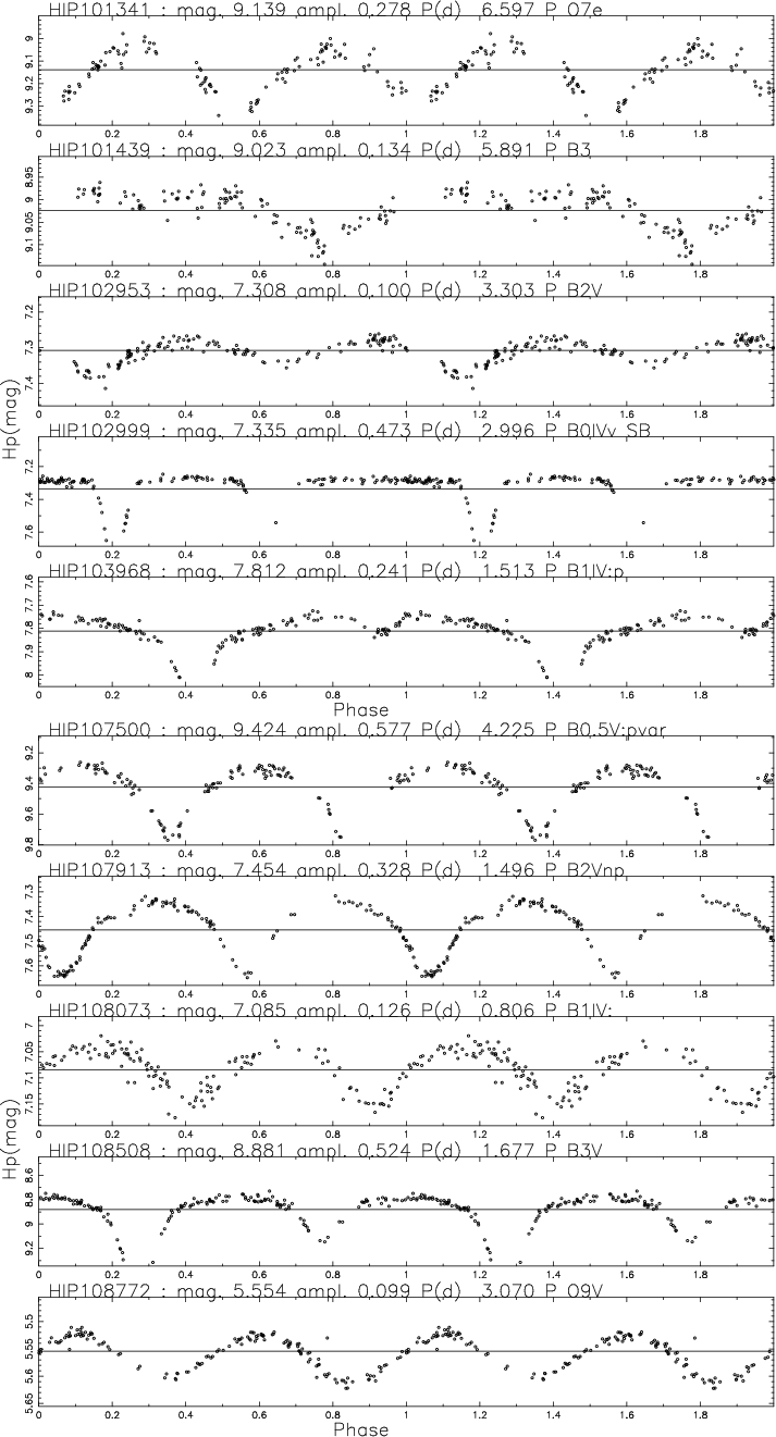
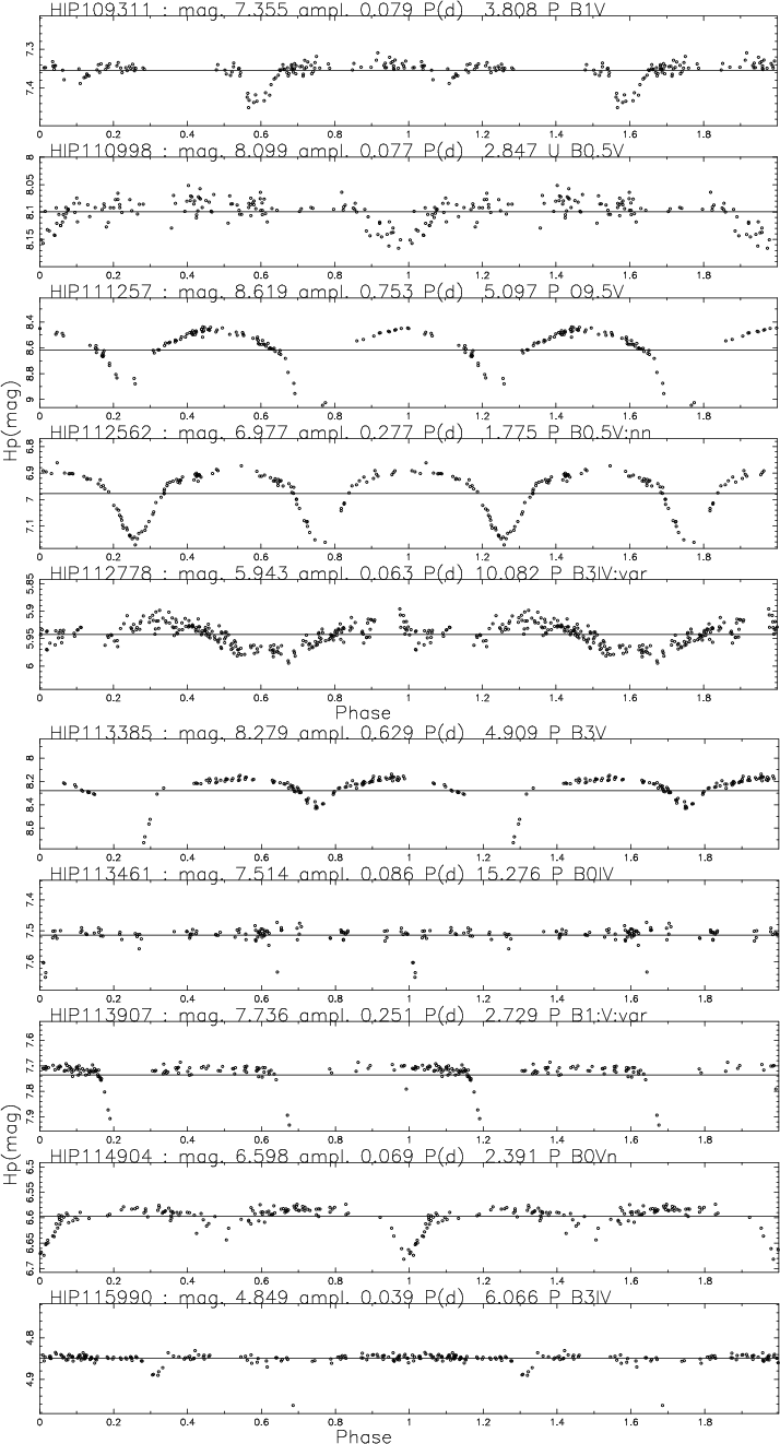
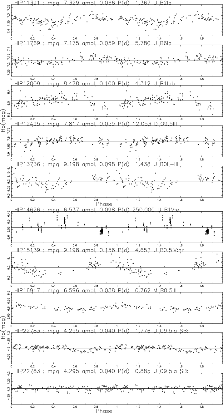
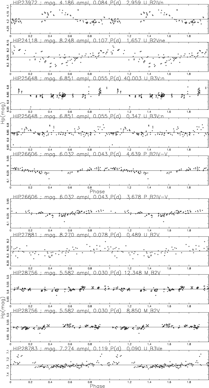
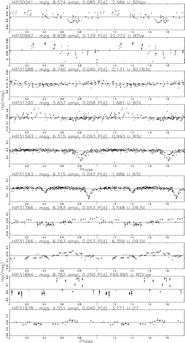
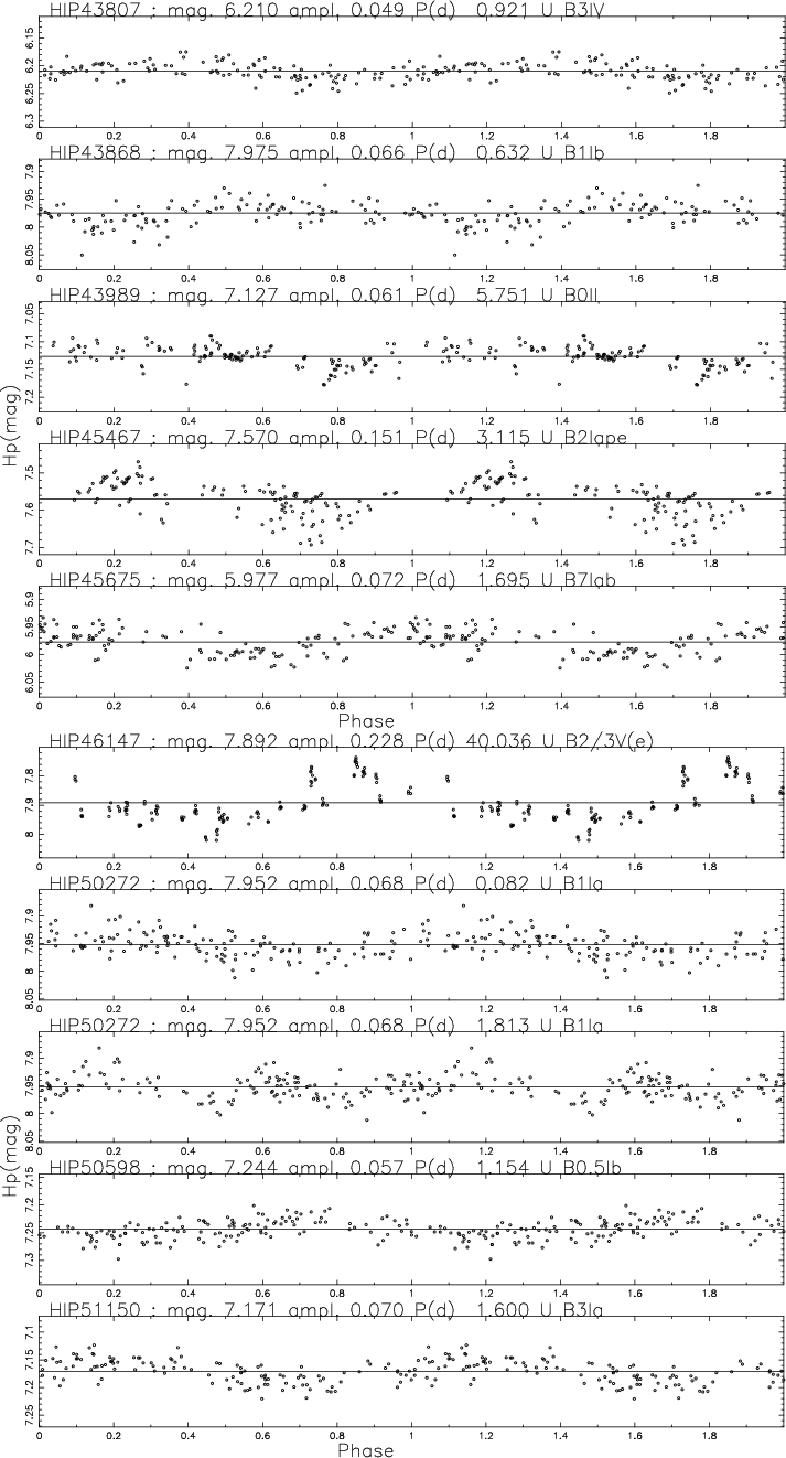
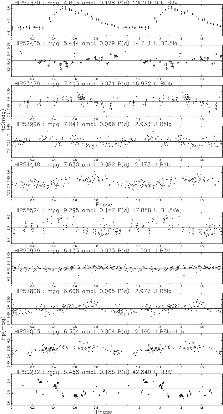
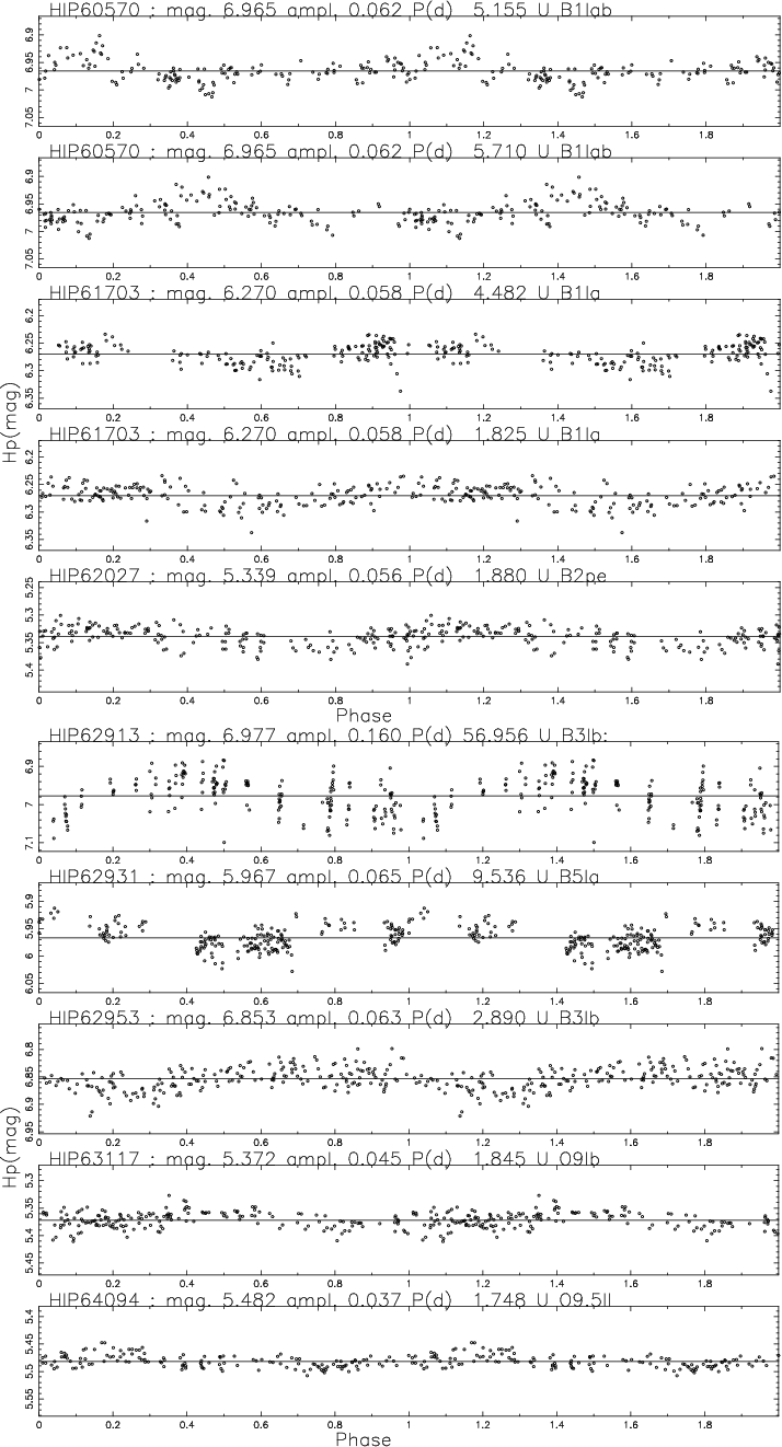
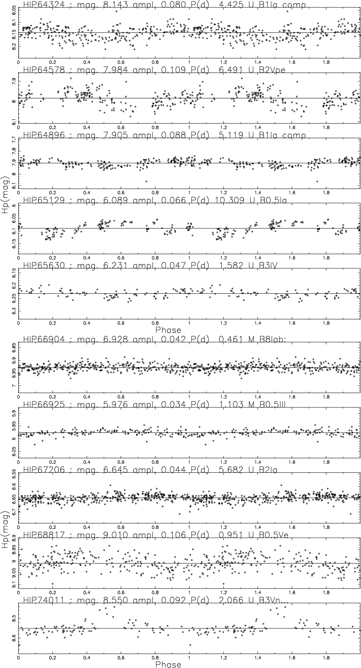
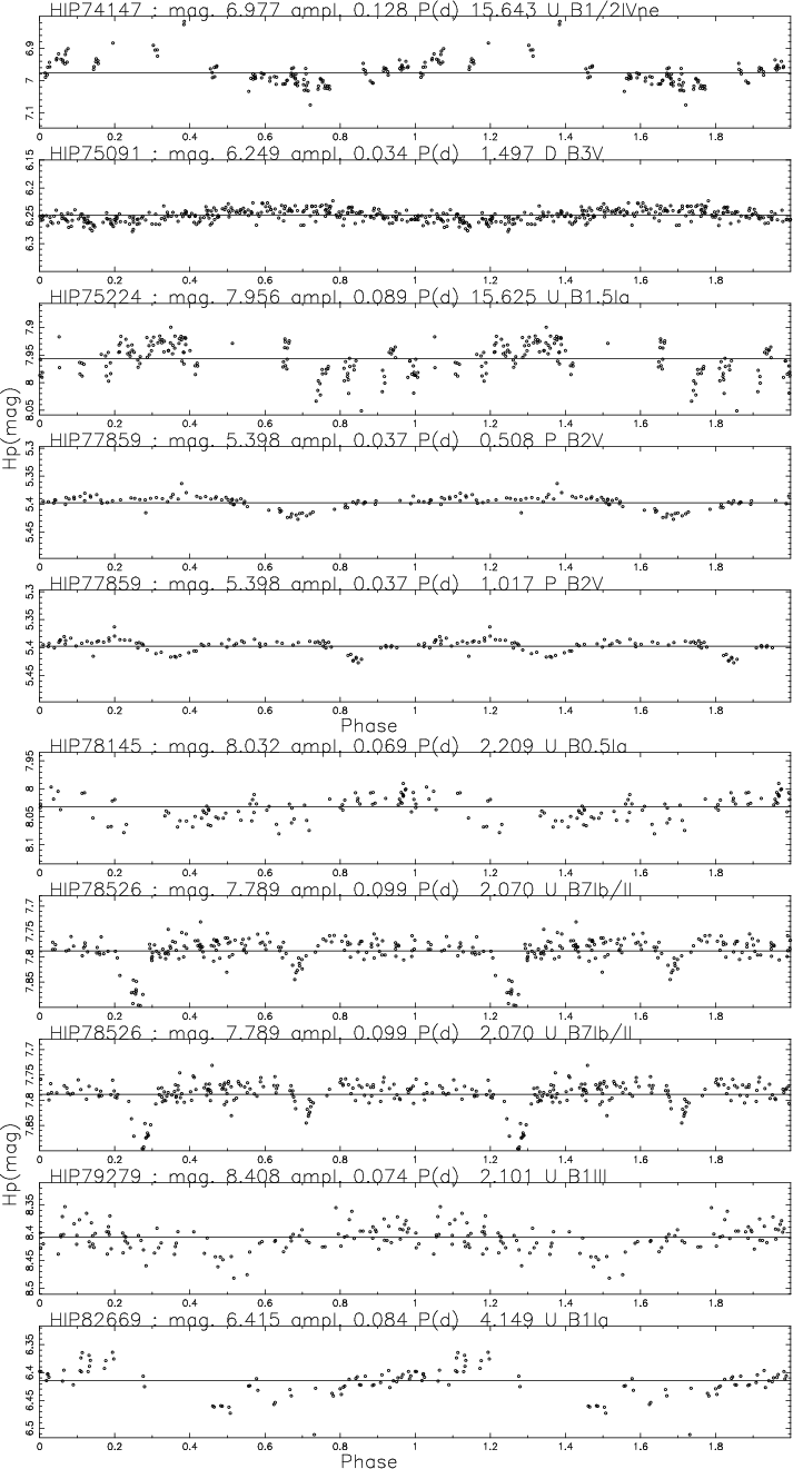
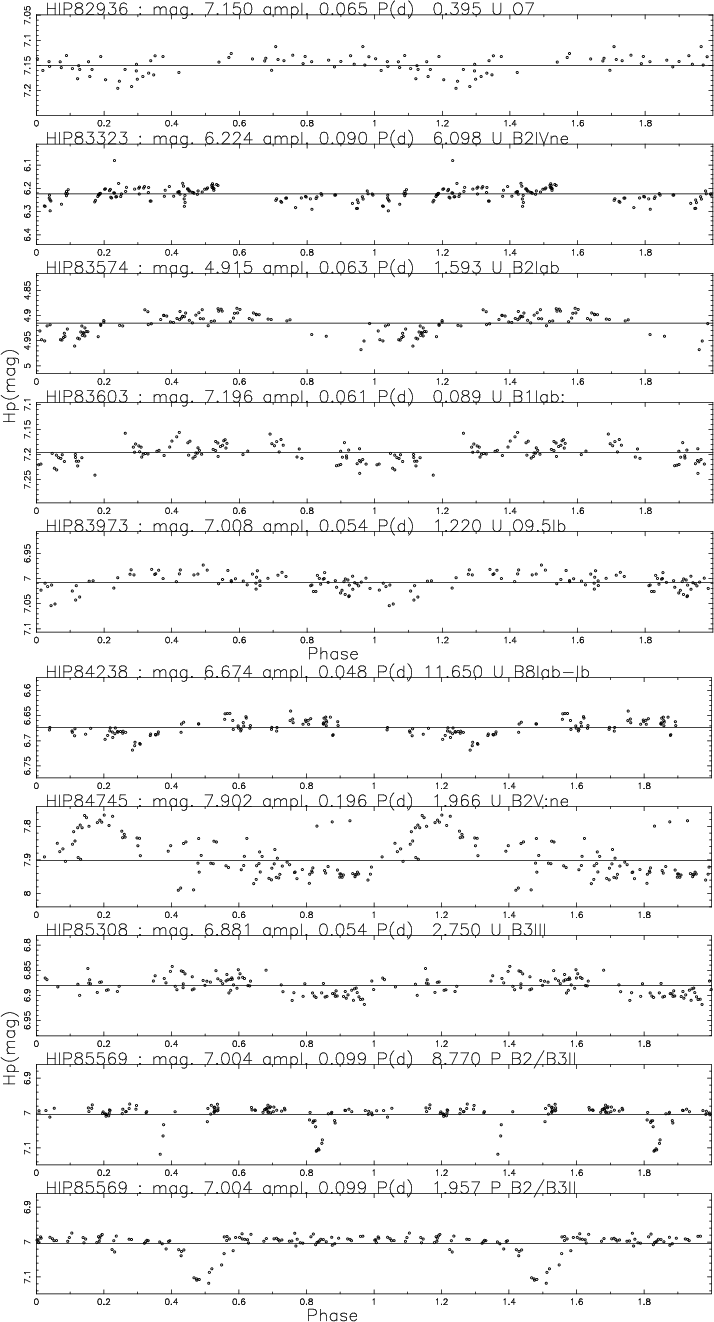
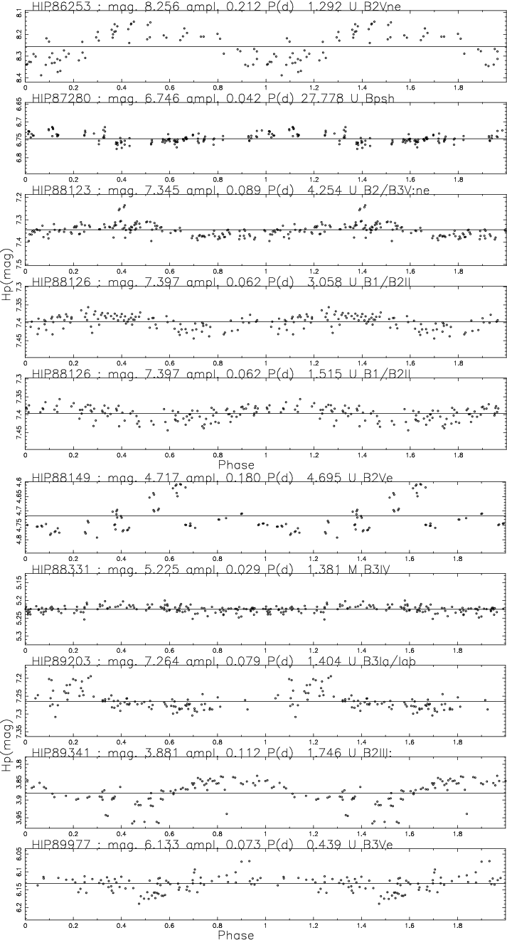
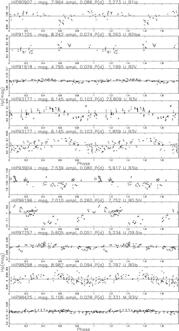
Appendix B: Lightcurves of variable OB stars from the Hipparcos catalog
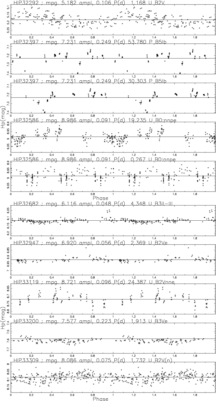
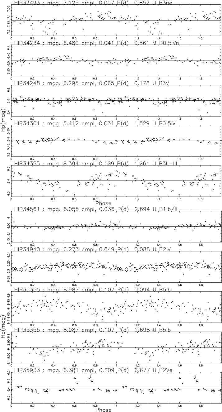
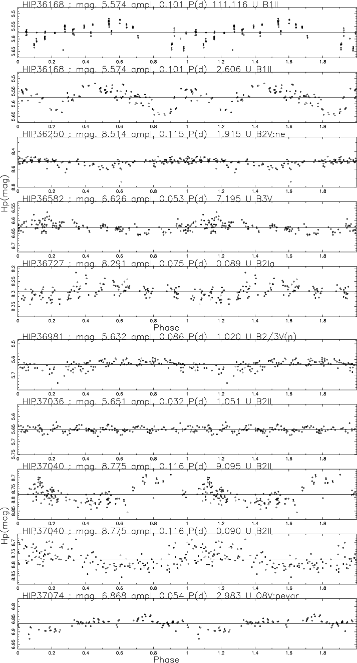
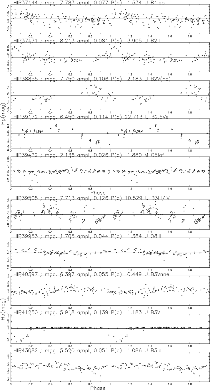
Above each lightcurve are found the HIPPARCOS number the ![]() magnitude, the mean amplitude (derived from this study) the phased period,
and the spectral type.
magnitude, the mean amplitude (derived from this study) the phased period,
and the spectral type.
B.1 Catalog of eclipsing binaries
|
Figure B.1:
This figure plots Hp mag. vs. Phase. Epoch is arbitrarily
JD-2 440 000=7800, which is the beginning of the HIPPARCOS observations. The Hp magnitude, mean amplitude and periods
are accurate to |
| Open with DEXTER | |
![]()
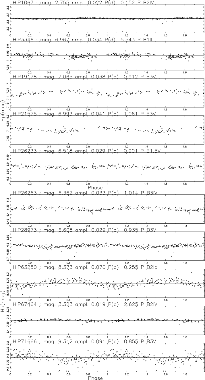
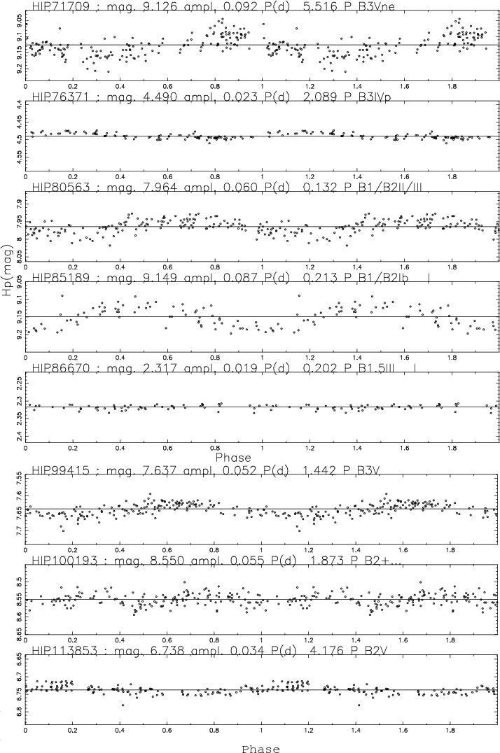
B.2 Catalog of new periodic variable stars
|
Figure B.2:
This figure plots Hp mag. vs. Phase. Epoch is arbitrarily
JD-2 440 000 = 7800, which is the beginning of the HIPPARCOS observations. The Hp magnitude, mean amplitude and periods
are accurate to |
| Open with DEXTER | |
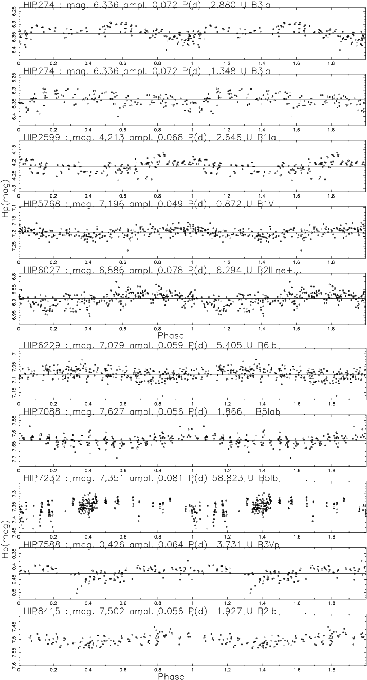
B.3 Catalog of non-included periodic variable stars
|
Figure B.3:
This figure plots Hp mag. vs. Phase. Epoch is arbitrarily
JD-2 440 000=7800, which is the beginning of the HIPPARCOS observations. The Hp magnitude, mean amplitude and periods
are accurate to |
| Open with DEXTER | |
B.4 Catalog of periodic stars below

|
Figure B.4:
This figure plots Hp mag. vs. Phase. Epoch is arbitrarily
JD-2 440 000=7800, which is the beginning of the HIPPARCOS observations. The Hp magnitude, mean amplitude and periods
are accurate to |
| Open with DEXTER | |
All Tables
Table 1: Selected stars.
Table 2: OB Stars in the 3 OB categories and corresponding statistics.
Table 3: OB eclipsing Stars in the 3 OB categories and corresponding statistics.
Table 4: OB eclipsing binaries of the HIPPARCOS catalog.
Table 5:
OBMS stars above the threshold ![]() .
.
Table 6:
OBe stars above the threshold ![]() .
.
Table 7:
OBSG stars above the threshold ![]() .
.
Table 8: OBSG star proportions in 3 mag bins.
Table 9:
Periodic stars not included
because of too many flagged points or below ![]() .
.
Table A.1: OB eclipsing binaries of the HIPPARCOS catalog.
Table A.2:
OBMS stars above the threshold ![]() .
.
Table A.3:
OBe stars above the threshold ![]() .
.
Table A.4:
OBSG stars above the threshold ![]() .
.
All Figures
|
|
Figure 1: Histogram of the magnitude of the stars in our sample. The cutoff near Hp=10 mag is completely artificial as it corresponds to the limit we chose for our sample. Note the steep decrease of the histogram above Hp=8 mag, where the sample is not complete. |
| Open with DEXTER | |
| In the text | |
|
|
Figure 2:
Distribution of the
internal error in our sample in the 3 intrinsic categories of stars from
Sect. 5. Squares represent OBMS stars, triangles OBe stars and circles OBSG stars. Overplotted in black is the calculated threshold |
| Open with DEXTER | |
| In the text | |
|
|
Figure 3:
Comparison
between the distribution in bins of magnitude and the
simulated results for the whole sample of OB stars superimposed in black
with the 3 intrinsic categories from Sect. 5. Bins are for Hp=[5, 5.5] ( left),
and Hp [9, 9.25] ( right). From top to bottom, the filled histograms
represent the number of OBMS, OBe and OBSG stars in the above-mentioned magnitude bins.
Note that there are a few points with a squared-amplitude that is off-scale in these diagrams;
these have not been shown for reasons of clarity. The solid line represents |
| Open with DEXTER | |
| In the text | |
|
|
Figure 4:
Variability threshold calculated for our sample. |
| Open with DEXTER | |
| In the text | |
|
|
Figure 5:
This figure is a representative extraction of our ``catalog of New
Periodic stars'' given in Appendix B2.
It plots Hp mag. vs. Phase. The epoch is arbitrarily taken as JD-2 440 000
=7800, which is the beginning of the HIPPARCOS observations. On top of each lightcurve are the HIPPARCOS
number, the Hp magnitude and mean amplitude calculated in this study, the period, variability flag and spectral
type from the HIPPARCOS data (periods can also be new ones). The Hp magnitude, mean amplitude and periods
are accurate to |
| Open with DEXTER | |
| In the text | |
|
|
Figure 6:
The four panels of this figure represent the distribution in magnitude for
the 3 intrinsic variability classes in 4 different situations. From top to bottom, OBMS stars, OBe stars and OBSG stars. a) The whole
sample of 2407 stars, b) the 1656 stars below |
| Open with DEXTER | |
| In the text | |
|
|
Figure 7:
This figure is the beginning of our ``catalog of Eclipsing Binaries''
given in Appendix B1. It contains 122 candidates; the remaining 5 are in
Appendix B3 and B4.
It plots Hp mag. vs. Phase. The epoch is arbitrarily taken as JD-2 440 000
=7800, which is the beginning of the HIPPARCOS observations. On top of each lightcurve are the HIPPARCOS
number, the Hp magnitude and mean amplitude calculated in this study, the period, variability flag and
spectral type from the
HIPPARCOS data (periods can also be new ones). The Hp magnitude, mean amplitude and periods
are accurate to |
| Open with DEXTER | |
| In the text | |
|
|
Figure 8: Eclipsing binaries: the upper left panel a) presents the log of the period (days) versus the log of the amplitude of the variations, while the upper right panel b) presents the histograms of the periods in the 3 intrinsic variability classes OBMS, OBe and OBSG. Squares represent OBMS stars, triangles OBe stars and circles OBSG stars. The lower left panel c) presents the histograms of the amplitude in the 3 intrinsic variability classes. The lower right panel d) presents the amplitude vs. Hp magnitude. |
| Open with DEXTER | |
| In the text | |
|
|
Figure 9:
Variable stars: from top to bottom, left to right. Colors and symbols are the same as in
Fig. 8. The first panel a) presents the
log of the period (days) versus the amplitude of the variations, while the second panel b) presents
the histograms of the periods in the 3 intrinsic variability classes
of OBMS, OBe and OBSG stars ( from bottom to top). The third panel c) presents the amplitude histograms
of the same 3 classes of variability, and the fourth d) is the same as Fig. 4
for the periodic stars above |
| Open with DEXTER | |
| In the text | |
|
|
Figure 10: Periodicities as a function of spectral type and luminosity class (cf. de Jager 1980). The tracks have been plotted according to the values of Vanbeveren et al. (1998). Symbol size is proportional to the amplitude of the variation. |
| Open with DEXTER | |
| In the text | |
|
|
Figure B.1:
This figure plots Hp mag. vs. Phase. Epoch is arbitrarily
JD-2 440 000=7800, which is the beginning of the HIPPARCOS observations. The Hp magnitude, mean amplitude and periods
are accurate to |
| Open with DEXTER | |
| In the text | |
![]()
|
|
Figure B.2:
This figure plots Hp mag. vs. Phase. Epoch is arbitrarily
JD-2 440 000 = 7800, which is the beginning of the HIPPARCOS observations. The Hp magnitude, mean amplitude and periods
are accurate to |
| Open with DEXTER | |
| In the text | |
|
|
Figure B.3:
This figure plots Hp mag. vs. Phase. Epoch is arbitrarily
JD-2 440 000=7800, which is the beginning of the HIPPARCOS observations. The Hp magnitude, mean amplitude and periods
are accurate to |
| Open with DEXTER | |
| In the text | |
|
|
Figure B.4:
This figure plots Hp mag. vs. Phase. Epoch is arbitrarily
JD-2 440 000=7800, which is the beginning of the HIPPARCOS observations. The Hp magnitude, mean amplitude and periods
are accurate to |
| Open with DEXTER | |
| In the text | |
Copyright ESO 2009
Current usage metrics show cumulative count of Article Views (full-text article views including HTML views, PDF and ePub downloads, according to the available data) and Abstracts Views on Vision4Press platform.
Data correspond to usage on the plateform after 2015. The current usage metrics is available 48-96 hours after online publication and is updated daily on week days.
Initial download of the metrics may take a while.