| Issue |
A&A
Volume 507, Number 2, November IV 2009
|
|
|---|---|---|
| Page(s) | 1107 - 1115 | |
| Section | Astronomical instrumentation | |
| DOI | https://doi.org/10.1051/0004-6361/200911875 | |
| Published online | 15 September 2009 | |
A&A 507, 1107-1115 (2009)
Double star orbits with semi-definite programming and alternatives
R. L. Branham, Jr.
Ianigla-CCT, Mendoza, C.C. 330, Mendoza, Argentina
Received 19 February 2009 / Accepted 7 September 2009
Abstract
Many methods have been proposed to calculate the apparent orbit of
a double star. Semi-definite programming (SDP) offers numerous
advantages, but is mathematically and computationally demanding. Aitken
suggested seventy years ago a simpler method that uses ordinary least
squares to calculate the coefficients of a conic section to represent
the apparent ellipse. But although simpler, this approach obfuscates
what is being minimized geometrically, and the calculated ellipse
appears inferior to that found from SDP. An alternative, proposed in
various investigations, uses nonlinear least squares to minimize the
square of the deviations in distance
and position angle. This method can suffer from divergence or
convergence, if it occurs, to a local rather than to a global minimum.
All three methods are applied to three binary
systems RST 4816, Wolf 424, and HR 466.
Key words: binaries: visual - methods: numerical
1 Introduction
The importance of double, or binary, stars to astronomy hardly needs
to be emphasized. A study of their orbits permits the calculation
of the sum of the masses of the components if we also have the parallax
of the system. The first stage of orbit computation consists of the
calculation of the apparent orbit of the secondary with respect to the
primary, usually the brighter of the two components. For visual
observations a measurement comprises: the separation between the
components, ![]() ;
the position angle
;
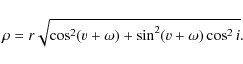
the position angle ![]() of the secondary with respect to the primary; and the time t of the observation.
of the secondary with respect to the primary; and the time t of the observation. ![]() and
and ![]() can be converted to rectangular coordinates
can be converted to rectangular coordinates
![]() and
and
![]() .
Then the equation for the apparent orbit, which the laws of dynamics specify as a conic section, generally an ellipse, becomes
.
Then the equation for the apparent orbit, which the laws of dynamics specify as a conic section, generally an ellipse, becomes
or in more symmetric notation
Several comments are in order. Equation (1) is homogeneous and has the trivial solution
I have developed a method, based on the new discipline of
semi-definite programming (SDP), that uses Eq. (2) to calculate a
non-trivial solution by maximizing the determinant of
proportional to the area of the ellipse, and guarantees that the solution be an ellipse by enforcing the condition that M be positive definite. The reduction algorithm also includes the calculation of the constant of areal velocity and can handle situations where radial velocities of the components are also available. SDP offers the advantages that: 1) it always converges when the data are reduced with the robust L1 criterion (minimize the sum of the absolute values of the residuals); 2) it converges to a global minimum of the reduction criterion; 3) the calculated apparent orbit is unique; and 4) when mixing astrometric with radial velocity data it is unnecessary to use the same norm with both classes of data. Although L1 is always advisable for the astrometric data, which usually show considerable scatter, it is sometimes preferable to use least squares with the radial velocities, frequently of higher quality than the astrometric data. I have used SDP to calculate the orbit of 24 Aquarii with only astrometric data (Branham 2006), to the same star with both astrometric and radial velocity data (radial velocities reduced with least squares) (Branham 2007), and to both interferometric and radial velocity data (radial velocities reduced with the L1 criterion) of Capella (
Despite the advantages of SDP, the method suffers from the drawbacks that it is complicated and demands considerable computational resources. Although I believe it should be the preferred method for orbit computation, many may prefer something simpler or something more closely related to what is observed directly, distance and position angle.
2 Alternatives to SDP: the Aitken method
A simple way to calculate an apparent orbit, mentioned in Aitken's
classic text on binary stars (1964, pp. 75-76), converts
Eq. (1) to a non-homogeneous equation by dividing through by l to obtain
This equation is easily solved by least squares for the coefficients A,B,H,G,F that can then be used in a standard method such as Kowalsky's (Smart 1962, Sect. 191) to calculate the true orbit. Several drawbacks, however, attend this simple application.
Let ![]() represent the matrix of the equations of condition in a least squares problem,
represent the matrix of the equations of condition in a least squares problem, ![]() the vector of the right-hand-side, and
the vector of the right-hand-side, and ![]() the vector of the solution. We seek a solution
the vector of the solution. We seek a solution
where ``
Although Eq. (4) is non-homogeneous, there is no guarantee that the solution must be an ellipse. One merely calculates the coefficients and hopes that they in fact represent an ellipse.
Then there arises the question of, exactly what is being minimized? The residuals from Eq. (5),
when minimized in the least squares sense,
But whatever criterion is used for the minimization, the constant of
areal velocity cannot be overlooked. This constant, denoted by C, is given by

Equation (4) can be amended to include the areal velocity, but one must be careful with the dimensions because Eq. (4) is dimensionless whereas Eq. (7) has dimensions of inverse time and must be multiplied by a time to assure compatibility. The amended equation can be written as
where t is a time. Equation (8) remains linear, permitting a quick solution for the variables A,B,H,G,F,C.
3 Alternatives to SDP: nonlinear least squares
Späth (1997) proposes an algorithm to minimize the perpendicular distance between the data point and the fitted ellipse. This differs from SDP's use of a line segment from the center to the data point, which will only be perpendicular to the ellipse when the eccentricity becomes zero. His algorithm allows for error in both x and y, but is nonlinear, requires numerous iterations, and takes no account of the constant of radial velocity. (To be fair to Späth, he considers only the problem of fitting ellipses to data, not the calculation of the apparent orbit of a double star.)
SDP's use of a line segment directed from the center of the
ellipse may seem somewhat artificial. With ellipses it seems more
natural to use the focus rather than the center of the ellipse. Both ![]() and
and ![]() can be referred to elliptical orbital elements of the true, not the apparent,
ellipse. These elements are: the period of revolution P; the time of periastron passage T; the eccentricity e; the semi-major axis
can be referred to elliptical orbital elements of the true, not the apparent,
ellipse. These elements are: the period of revolution P; the time of periastron passage T; the eccentricity e; the semi-major axis
![]() ;
the node
;
the node ![]() ;
the inclination i; and the perihelion
;
the inclination i; and the perihelion ![]() .
See Aitken (1964, pp. 75-80) for more discussion of the elements and the relation between the apparent and the true orbit. If v is the true anomaly, calculated from the eccentric anomaly that in turn is found from Kepler's equation,
.
See Aitken (1964, pp. 75-80) for more discussion of the elements and the relation between the apparent and the true orbit. If v is the true anomaly, calculated from the eccentric anomaly that in turn is found from Kepler's equation, ![]() and
and ![]() are related to the orbital elements by
are related to the orbital elements by
Many prefer to minimize the deviations in
Table 1: Observational data for double star RS 4816.
Should one wish to perform a differential correction, equations for calculating the partial derivatives of ![]() and
and ![]() with respect to the orbital elements are given in, among other sources, Aitken (1964, p. 111) and Plummer (1960, p. 112). When using these partial derivatives one
must avoid two pitfalls. Regarding the first consider the partial
with respect to the orbital elements are given in, among other sources, Aitken (1964, p. 111) and Plummer (1960, p. 112). When using these partial derivatives one
must avoid two pitfalls. Regarding the first consider the partial
![]() .
One should use the theoretically calculated
.
One should use the theoretically calculated ![]() from Eq. (9) rather than the observed
from Eq. (9) rather than the observed ![]() .
This is also true for
.
This is also true for ![]() .
The observed
.
The observed ![]() can
involve substantial error, which will propagate into the partial
derivative. For the example of the next section there is a
27% difference in the norms of the vectors of the partial
derivatives of
can
involve substantial error, which will propagate into the partial
derivative. For the example of the next section there is a
27% difference in the norms of the vectors of the partial
derivatives of ![]() .
As for the second, depending on the quadrant of
.
As for the second, depending on the quadrant of ![]() and
and
![]() ,
,
![]() can become negative. If this
happens, it should be made positive, and also in the partials where it
appears. Otherwise, the observed minus calculated value, (O-C), becomes
large, so large as to possibly destroy convergence. Alternatively,
one could combine the
can become negative. If this
happens, it should be made positive, and also in the partials where it
appears. Otherwise, the observed minus calculated value, (O-C), becomes
large, so large as to possibly destroy convergence. Alternatively,
one could combine the ![]() of Eq. (9) with a companion equation,
of Eq. (9) with a companion equation,
![]() ,
into a single expression
,
into a single expression
The problem of a negative
Rather than use ![]() and
and ![]() independently and minimize (
independently and minimize (
![]() ,
one might feel that the two should be combined into a single expression,
,
one might feel that the two should be combined into a single expression,
and F2 minimized. The partial derivatives of F with respect to the orbital elements can be calculated with Maple. Minimization of F2, however, fails because the matrix of equations of condition derived from Eq. (11) is singular, as a singular value decomposition shows.
4 Examples
I will study three systems, RST 4816, Wolf 424, and HR 466, to show how the SDP approach works, and seems to work well, when applied to binary systems. The first system, RST 4816, was chosen because, although there are few observations of the system, they cover the entire orbit. The second, Wolf 424, because there has been evidence that the two components may be brown dwarfs, and one should, if possible, confirm or reject the possibility. The third because Pourbaix (1996) has published an orbit for this system that also includes radial velocities. Because Pourbaix's method, unlike most nonlinear least squares techniques, almost guarantees convergence to a global minimum, one can compare it with what SDP gives, also a global minimum albeit in the L1 norm.
The first system, WDS 06362-3608 (RST 4816, HIP 31547), was discovered by Rossiter in 1942 (Rossiter 1944), who gave visual magnitudes of 7.9 for each component. The Washington Double Star Catalog (http://ad.usno.navy.mil/wds) provides data for this binary:
![]() ,
,
![]() ,
magnitude and spectral type of primary 7.77 G2 V, and
for the secondary 8.61 G3 V. According to Van Leeuwen's
reduction of the Hipparcos data, the parallax
,
magnitude and spectral type of primary 7.77 G2 V, and
for the secondary 8.61 G3 V. According to Van Leeuwen's
reduction of the Hipparcos data, the parallax ![]() of the system is 25.39
of the system is 25.39 ![]() 0.43 mas (Van Leeuwen 2007).
The small number of observations, which nevertheless cover the entire
orbit, assure that differences between the different reduction methods
to be employed will not be minimized because of the law of large
numbers. Table 1 shows the relevant data for RST 4816, including the
type of observation, the t needed in Eq. (8) and
0.43 mas (Van Leeuwen 2007).
The small number of observations, which nevertheless cover the entire
orbit, assure that differences between the different reduction methods
to be employed will not be minimized because of the law of large
numbers. Table 1 shows the relevant data for RST 4816, including the
type of observation, the t needed in Eq. (8) and
![]() ;
the former is taken as time in days from the mean time of the observations and the latter as radians per day. To find
;
the former is taken as time in days from the mean time of the observations and the latter as radians per day. To find
![]() I graph year versus
I graph year versus ![]() ,
adding or subtracting multiples of 360
,
adding or subtracting multiples of 360![]() from
from ![]() to produce a continuous curve, pass a polynomial through the data points, and then differentiate the polynomial.
to produce a continuous curve, pass a polynomial through the data points, and then differentiate the polynomial.
Upon examining Fig. 2 it appears as if there may be greater scatter in the observations for 1964-1996. The position angle ![]() in particular seems erratic and varies between 33
in particular seems erratic and varies between 33
![]() 7 and 111
7 and 111
![]() 8. Given the closeness in magnitude of the two components, could this be an instance of assigning
8. Given the closeness in magnitude of the two components, could this be an instance of assigning ![]() to the wrong quadrant? Perhaps, but this variation is statistically
insignificant. From the SDP solution in the next section if we look at
the residuals in position angle, the mean of the absolute values of the
other than 1964-1966 residuals is 0.288 rad, the mean of the
1964-1966 residuals is 0.357 rad. The respective standard
deviations are 0.288 and 0.442. At the 95% confidence level
we must reject the hypothesis that the two means are statistically
different.
to the wrong quadrant? Perhaps, but this variation is statistically
insignificant. From the SDP solution in the next section if we look at
the residuals in position angle, the mean of the absolute values of the
other than 1964-1966 residuals is 0.288 rad, the mean of the
1964-1966 residuals is 0.357 rad. The respective standard
deviations are 0.288 and 0.442. At the 95% confidence level
we must reject the hypothesis that the two means are statistically
different.
From the data in Table 1 I calculate two solutions using OLS, one with and one without the areal velocity constant. Figure 1 shows the data points and the calculated ellipses. One sees that the two ellipses differ and that including or not including the areal velocity constant makes a significant difference. Given this, no further mention will be made of calculating the apparent ellipse without the constant of areal velocity.
![\begin{figure}
\par\includegraphics[height=7.1cm,width=8cm,clip]{Fig1.eps}
\end{figure}](/articles/aa/full_html/2009/44/aa11875-09/img45.png)
|
Figure 1: OLS solution with (solid line) and without (dash-dot line) areal velocity constant. |
| Open with DEXTER | |
5 SDP, OLS, and TLS solutions
To calculate an SDP solution one needs
![]() .
This has already been given in Table 1 and is obtained by plotting year versus
.
This has already been given in Table 1 and is obtained by plotting year versus ![]() ,
Fig. 2. Then multiples of 360
,
Fig. 2. Then multiples of 360![]() are added or subtracted to produce a more or less continuous curve, Fig. 3. A cubic polynomial gives a good fit to this curve, which is differentiated to produce a curve of year versus
are added or subtracted to produce a more or less continuous curve, Fig. 3. A cubic polynomial gives a good fit to this curve, which is differentiated to produce a curve of year versus
![]() ,
Fig. 4. With these data my SDP algorithm calculates a solution for the apparent ellipse, shown in Table 2,
along with the orbital elements found from Kowalsky's method. The
period and time of periastron passage as well as the mean errors for
the orbital elements are calculated in the
manner outlined in Branham (2007).
,
Fig. 4. With these data my SDP algorithm calculates a solution for the apparent ellipse, shown in Table 2,
along with the orbital elements found from Kowalsky's method. The
period and time of periastron passage as well as the mean errors for
the orbital elements are calculated in the
manner outlined in Branham (2007).
![\begin{figure}
\par\includegraphics[height=7.4cm,width=8cm,clip]{Fig2.eps}
\end{figure}](/articles/aa/full_html/2009/44/aa11875-09/img46.png)
|
Figure 2: Year versus theta. |
| Open with DEXTER | |
![\begin{figure}
\par\includegraphics[height=7.2cm,width=8cm,clip]{Fig3.eps}
\end{figure}](/articles/aa/full_html/2009/44/aa11875-09/img47.png)
|
Figure 3: Year versus theta after adding/substracting multiples of 360 degrees. |
| Open with DEXTER | |
![\begin{figure}
\par\includegraphics[height=7.4cm,width=8cm,clip]{Fig4.eps}
\vspace*{5mm}
\end{figure}](/articles/aa/full_html/2009/44/aa11875-09/img48.png)
|
Figure 4: Year versus thetadot in radians/day. |
| Open with DEXTER | |
The OLS solution in Table 3 uses Eq. (8), with the mean errors calculated in the usual way. Table 4's TLS solution follows the prescription given in Branham (2001), with all of the columns of P and the vector ![]() containing error. Should one wish to use, for whatever reason,
Eq. (4) in lieu of Eq. (8), then one must make a significant
modification. Seeing as the right-hand-side is error-free, account must
be taken of this. Van Huffel & Vandewalle (1991, Sect. 3.6.2) recommend estimating the absolute sizes of the errors in
containing error. Should one wish to use, for whatever reason,
Eq. (4) in lieu of Eq. (8), then one must make a significant
modification. Seeing as the right-hand-side is error-free, account must
be taken of this. Van Huffel & Vandewalle (1991, Sect. 3.6.2) recommend estimating the absolute sizes of the errors in ![]() and
and ![]() scaling so that the estimates are as equal as possible. I have found that in practice scaling each column of
scaling so that the estimates are as equal as possible. I have found that in practice scaling each column of ![]() and
and ![]() to have unit Euclidean norm works well. With an error-free
to have unit Euclidean norm works well. With an error-free ![]() ,
one merely omits the scaling of this vector. The calculation of the
mean errors is somewhat more complicated. I have discussed how to
estimate TLS mean errors (Branham 1999). In Eq. (8) of that publication set the column of the covariance matrix corresponding to the vector
,
one merely omits the scaling of this vector. The calculation of the
mean errors is somewhat more complicated. I have discussed how to
estimate TLS mean errors (Branham 1999). In Eq. (8) of that publication set the column of the covariance matrix corresponding to the vector
![]() to zero.
to zero.
I also tried to calculate a nonlinear least squares solution using a
differential correction with partial derivatives taken from Plummer (1960)
and first approximation taken from the OLS solution. The iterates,
however, failed to converge. Nor did they converge if I used the TLS or
the SDP solution as the first approximation. Zadunaisky &
Pereya (1965) have proven that
lack of convergence in differential corrections is caused by:
1) a poor initial approximation to the solution;
2) a poorly conditioned matrix of equations of condition;
3) the presence of large residuals. Here the initial
approximations are good, nor is the condition number of the matrix,
4.6 ![]() 103,
high. The problem, therefore, must be caused by one or more large
residuals. The median of the absolute values of the residuals in
103,
high. The problem, therefore, must be caused by one or more large
residuals. The median of the absolute values of the residuals in ![]() is 0
is 0
![]() 040 versus a median
040 versus a median ![]() of 0
of 0
![]() 137; for
137; for ![]() the corresponding numbers are 37
the corresponding numbers are 37
![]() 08 and 111
08 and 111
![]() 80. The residuals, therefore, are large, and this must be the cause of the divergence of the iterates.
80. The residuals, therefore, are large, and this must be the cause of the divergence of the iterates.
Table 2: SDP solution for RST 4816.
Table 3: OLS solution.
Table 4: TLS solution.
Table 2 shows the solution from SDP and Tables 3 and 4 the two least squares solutions, one from OLS, and one from TLS. For all three of these the solution was iterated once. The weighting factors come from the biweight, the same weighting used in Branham (2007, 2008): scale the post-fit residuals by the median of the absolute values of the residuals and calculate weighting factors wi by:
The advantages of the biweight are: it is impersonal, no subjective impressions affect the weighting; it also recognizes an important fact from the central limit theorem of statistics, that smaller residuals are more probable than larger ones and assigns higher weight to small residuals. Figure 5 graphs the ellipses from the two least squares solutions and Fig. 6 shows the SDP solution compared with the OLS solution. Figure 7 graphs the weights calculated from the SDP solution and Eq. (12) versus the year.
![\begin{figure}
\par\includegraphics[height=7.1cm,width=8cm,clip]{Fig5.eps}
\end{figure}](/articles/aa/full_html/2009/44/aa11875-09/img65.png)
|
Figure 5: Ellipses from OLS (solid line) and TLS (dash-dot line). |
| Open with DEXTER | |
![\begin{figure}
\par\includegraphics[height=7.2cm,width=8cm,clip]{Fig6.eps}
\end{figure}](/articles/aa/full_html/2009/44/aa11875-09/img66.png)
|
Figure 6: Ellipses from SDP ( lower) and OLS ( upper). |
| Open with DEXTER | |
If MA and MB represent the masses of the components in units of the solar mass ![]() ,
from Kepler's third law their sum M is
,
from Kepler's third law their sum M is
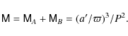
To find a mean error for the sum of the masses we need a covariance matrix, which can be calculated from:
From Eqs. (13) and (14) we calculate for the SDP solution
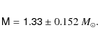
Because we have no fractional mass available, it is impossible to calculate the individual masses. One can say that the sum of the masses is consistent with what one would expect from G dwarfs.
6 Wolf 424 and HR 466
Having given a detailed presentation for RST 4816, I will confine myself to summary results for Wolf 424 and HR 466. These systems, moreover, have already been studied in detail by others, using techniques different from SDP. Torres et al. (1999), among others, have studied Wolf 424, but since 1999 additional observations have been made, including five high quality observations sent me by Dr. Sergi Hildebrandt of the Instituto de Astrofísica de las Canarias (personal communication). Given the high eccentricity of the apparent orbit, 0.99, this binary will be a good test of the applicability of the SDP method to high eccentricity systems. Whether the components are brown dwarfs, as some suspect, should also be investigated. Jorge Prieto, also of the Instituto, is planning a more detailed study of this particular binary (personal communication).
![\begin{figure}
\par\includegraphics[height=7.3cm,width=8cm,clip]{Fig7.eps}
\end{figure}](/articles/aa/full_html/2009/44/aa11875-09/img73.png)
|
Figure 7: Weights for SDP solution. |
| Open with DEXTER | |
For Wolf 424 (Gliese 473, WDS 12335+0901) there are
65 observations available, from 1938 to 2009, of which 60 come
from the Washington Double Star Catalog (http://ad.usno.navy.mil/wds), which gives this data for the binary:
![]() ,
,
![]() ,
with magnitudes of 12.6 for both the primary and the secondary. According to Torres et al. (1999) both components are late-type M dwarfs, combined spectral type M5.5 Ve, with parallax
,
with magnitudes of 12.6 for both the primary and the secondary. According to Torres et al. (1999) both components are late-type M dwarfs, combined spectral type M5.5 Ve, with parallax
![]()
![]() 0.46 mas. Dr. Hildebrandt adds five FastCam observations:
0.46 mas. Dr. Hildebrandt adds five FastCam observations:
Table 5: FastCam observations of Wolf 424.
Using the same methodology as applied to RST 4816 for the SDP solution, I calculate an orbit for Wolf 424, given in Table 6 and shown graphically in Fig. 8. For the sake of comparison the Torres et al. (1999) orbit is also shown in Table 6. Equation (12) calculates the weights, which vary from a minimum of 0.200 to a maximum of 1.000 with a median of 0.911.
Table 6: SDP solution for Wolf 424.
![\begin{figure}
\par\includegraphics[height=7.4cm,width=8cm,clip]{Fig8.eps}
\end{figure}](/articles/aa/full_html/2009/44/aa11875-09/img85.png)
|
Figure 8: Ellipse for Wolf 424: SDP. |
| Open with DEXTER | |
The sum of the masses comes from Eq. (12) and the individual masses from multiplying the sum by the mass fraction ![]() .
If we take Torres et al.'s (1999) value for the parallax and the mass fraction, 0.477
.
If we take Torres et al.'s (1999) value for the parallax and the mass fraction, 0.477 ![]() 0.008, the masses become:
0.008, the masses become:
![]()
![]() 0.070
0.070
![]() ;
;
![]()
![]() 0.078
0.078
![]() .
These masses are far above the substellar limit of 0.08
.
These masses are far above the substellar limit of 0.08
![]() and
thus give no indication that either of the components is a brown dwarf.
The corresponding masses from Torres et al. are
and
thus give no indication that either of the components is a brown dwarf.
The corresponding masses from Torres et al. are
![]()
![]() 0.011
0.011
![]() and
and
![]()
![]() 0.010
0.010
![]() ,
lower but still above the substellar limit.
,
lower but still above the substellar limit.
The residuals show a good distribution about the orbit,
34 positive residuals and 31 negative, although with
18 runs out of an expected 33 there are obviously systematic
errors present. But interestingly, the Torres et al. (1999) solution also shows a deficiency of runs, 17 runs out of an expected 26 in ![]() and 15 runs out of an expected 28 in
and 15 runs out of an expected 28 in ![]() .
It thus appears as if the weighting function of Eq. (12)
works as well as assigning higher weight to certain classes of
observation, such as the speckle interferometric data, the procedure
followed by Torres et al.
(1999). One can even aver that the high weight assigned to some classes of observation distorts the solution. Figure 9
shows, on the upper portion, the fit to the visual and photographic
observations and on the lower portion the fit to the speckle and
Hipparcos Fine Guidance Sensor observations. It is evident that
high weight of the latter forces the solution to pass close to these
observations and displace the entire ellipse away from the visual and
photographic observations. This example also shows that the SDP
approach works well even with systems of high eccentricity of the
apparent orbit, 0.9899
.
It thus appears as if the weighting function of Eq. (12)
works as well as assigning higher weight to certain classes of
observation, such as the speckle interferometric data, the procedure
followed by Torres et al.
(1999). One can even aver that the high weight assigned to some classes of observation distorts the solution. Figure 9
shows, on the upper portion, the fit to the visual and photographic
observations and on the lower portion the fit to the speckle and
Hipparcos Fine Guidance Sensor observations. It is evident that
high weight of the latter forces the solution to pass close to these
observations and displace the entire ellipse away from the visual and
photographic observations. This example also shows that the SDP
approach works well even with systems of high eccentricity of the
apparent orbit, 0.9899 ![]() 0.0029 for Wolf 424.
0.0029 for Wolf 424.
![\begin{figure}
\par\includegraphics[height=7.2cm,width=8cm,clip]{Fig9.eps}
\end{figure}](/articles/aa/full_html/2009/44/aa11875-09/img92.png)
|
Figure 9: Ellipses from Torres et al. solution. |
| Open with DEXTER | |
An OLS solution for this system, including the areal velocity constant as an unknown, once again, as with RST 4816, becomes inferior, giving only 11 positive residuals, 54 negative residuals, and 10 runs out of an expected 33. Figure 10 graphs the ellipse. And, once again, differential corrections fail to converge, most likely for the same reason: the presence of large residuals. One can, of course, use nonlinear least squares, what Torres et al. (1999) do, but then one must demonstrate that the minimum calculated corresponds to a global minimum. For the SDP solution given here there is no doubt about the minimum being global, albeit in the L1 norm.
![\begin{figure}
\par\includegraphics[height=7.2cm,width=8cm,clip]{Fig10.eps}
\end{figure}](/articles/aa/full_html/2009/44/aa11875-09/img93.png)
|
Figure 10: Ellipse for Wolf 424: OLS. |
| Open with DEXTER | |
My final example, HR 466 (WDS 1376-0924, ![]() =
=
![]() ,
,
![]() =
=
![]() ,
with magnitudes of 6.8 for the primary and 7.2 for the secondary), was
selected because Pourbaix (1998)
has published an orbit for this binary that includes radial velocities.
His method, moreover, because it is based on simulated annealing,
converges with high probability to a global minimum, although in the
least squares norm. Poubaix uses 28 high quality
CHARA interferometric observations and eight double line radial
velocities. I requested all of the observations,
80 altogether, taken from, once again, the Washington Double Star
Catalog (http://ad.usno.navy.mil/wds)
and covering the years 1934 to 2007. For the final solution,
however, for reasons explained shortly, only 44 speckle
observations made between 1976 and 2007 were used.
Equation (12) calculated the weights for the interferometric
observations, which vary from 0 for three of the observation
to 1.000 with a median of 0.991, and also for separate
weights, which vary from 0.823 to 0.996 with a median
of 0.911, for the radial velocities. Table 7 shows this solution, and for comparison, Pourbaix's. Figure 11 plots the solution for the interferometric observations and Fig. 12
for the radial velocities. The interferometric observations are
distributed well about the ellipse, with 21 positive residuals and
23 negative. There are 18 runs out of an expected 22,
slightly on the low side but still fairly random. To be precise,
from a strictly statistical point of view there is a 22.6% chance
that the residuals are random. The fit to the radial velocities is less
satisfactory, with four runs out of an expected eight. The parallax of
the system agrees fairly well with van Leeuwen's 24.77
,
with magnitudes of 6.8 for the primary and 7.2 for the secondary), was
selected because Pourbaix (1998)
has published an orbit for this binary that includes radial velocities.
His method, moreover, because it is based on simulated annealing,
converges with high probability to a global minimum, although in the
least squares norm. Poubaix uses 28 high quality
CHARA interferometric observations and eight double line radial
velocities. I requested all of the observations,
80 altogether, taken from, once again, the Washington Double Star
Catalog (http://ad.usno.navy.mil/wds)
and covering the years 1934 to 2007. For the final solution,
however, for reasons explained shortly, only 44 speckle
observations made between 1976 and 2007 were used.
Equation (12) calculated the weights for the interferometric
observations, which vary from 0 for three of the observation
to 1.000 with a median of 0.991, and also for separate
weights, which vary from 0.823 to 0.996 with a median
of 0.911, for the radial velocities. Table 7 shows this solution, and for comparison, Pourbaix's. Figure 11 plots the solution for the interferometric observations and Fig. 12
for the radial velocities. The interferometric observations are
distributed well about the ellipse, with 21 positive residuals and
23 negative. There are 18 runs out of an expected 22,
slightly on the low side but still fairly random. To be precise,
from a strictly statistical point of view there is a 22.6% chance
that the residuals are random. The fit to the radial velocities is less
satisfactory, with four runs out of an expected eight. The parallax of
the system agrees fairly well with van Leeuwen's 24.77 ![]() 0.71 mas (2007).
0.71 mas (2007).
Table 7: SDP solution for HR466.
![\begin{figure}
\par\includegraphics[height=7.1cm,width=8cm,clip]{Fig11.eps}
\end{figure}](/articles/aa/full_html/2009/44/aa11875-09/img116.png)
|
Figure 11: Ellipse for HR466. |
| Open with DEXTER | |
![\begin{figure}
\par\includegraphics[height=7.2cm,width=8cm,clip]{Fig12.eps}
\end{figure}](/articles/aa/full_html/2009/44/aa11875-09/img117.png)
|
Figure 12: Radial velocities for HR466: observed (asterisk), calculated (dot). |
| Open with DEXTER | |
An OLS solution yields less than satisfactory results: 18 postive residuals and 26 negative with 12 runs out of an expected 22. It appears as if, once again, a linear least squares solution as recommended by Aitken just does not work well. For this reason no differential correction was attempted.
Now I may address the question why the solution from the
speckle observations should be accepted rather than one based on all of
the observations. The latter finds on orbit less eccentric,
eccentricity of the true orbit of 0.678, and with considerably
smaller semi-major axis, 0
![]() 225.
Although statistics seem to confirm a good fit, 40 positive
residuals and 40 negative, there is a noticeable deficiency of
runs, 24 out of an expected 40. When one calculates the
parallax of the
system,
225.
Although statistics seem to confirm a good fit, 40 positive
residuals and 40 negative, there is a noticeable deficiency of
runs, 24 out of an expected 40. When one calculates the
parallax of the
system,
![]()
![]() 1.88 mas, a discrepancy with the van Leeuwen parallax emerges.
It seems difficult to reconcile such a small parallax with van
Leeuwen's 24.77 mas. The parallax is also discrepant with regard
to what Pourbaix and others have found for this system. Given this
external evidence it appears as if systematic errors in the non-speckle
observations have
compromised the orbit.
1.88 mas, a discrepancy with the van Leeuwen parallax emerges.
It seems difficult to reconcile such a small parallax with van
Leeuwen's 24.77 mas. The parallax is also discrepant with regard
to what Pourbaix and others have found for this system. Given this
external evidence it appears as if systematic errors in the non-speckle
observations have
compromised the orbit.
7 Discussion
To confine our attention first to RST 4816, the divergence of the
nonlinear least squares solution is disquieting. Although one has some
control over the initial approximation and the condition number of the
matrix of the equations of condition, which can usually be lowered by
an adequate scaling strategy such as reducing each column of the matrix
to unit Euclidean norm, one has little control over the residuals. The
nonlinear least squares method has been used successfully,
as Barlow et al. (1993)
demonstrate. The fact, however, that it can fail, versus SDP's
guaranteed convergence, should give one pause, even though minimizing
deviations in ![]() and
and ![]() may seem intuitively more appealing than minimizing a line segment from the center of the ellipse to the data point.
may seem intuitively more appealing than minimizing a line segment from the center of the ellipse to the data point.
Several facts emerge from a study of Tables 2-4 and Figs. 5 and 6. The two least squares solution do not differ greatly from one another, although the TLS mean errors are in general higher than those from OLS. This is true in general; see Branham (1999). But given the greater complexity of a TLS solution, especially should one opt for an error-free right-hand-side, it hardly appears worthwhile to go to the extra effort to calculate a TLS solution versus the relatively easy OLS solution.
Both least squares solutions give an ellipse with a long semi-major axis, but significantly less eccentric than the SDP solution. The distribution of the observations about the ellipse is superior with the SDP solution, seven observations outside of the ellipse, six within. Least squares, on the other hand, gives four observations outside of the ellipse, nine within, despite what a runs test indicates for the randomness of the residuals. With thirteen observations we would expect 6 or 7 runs with a standard deviation of 1.8. Applied to the three solutions the runs test gives for OLS nine runs, for TLS seven runs, and for SDP six. The SDP runs agree well with what is observed in Fig. 6 but are far off the mark for the OLS runs. This, however, is a consequence of how we define the residuals. With SDP the residuals have a clear geometric interpretation whereas with least squares they arise from the solution of a linear system where the relationship between the fitted ellipse and the minimization criterion is highly convoluted. With OLS, for example, the residuals given by Eq. (6) bear no obvious relation to the ellipses shown in Fig. 5.
In addition to the runs test, it may be instructive to see how the
SDP solution fares with a comparison between the calculated orbit
and what is actually observed in the x and y coordinates and in ![]() and
and ![]() .
Although the SDP residuals are minimized with respect to what is
called in differential geometry the ``metric distance'', which depends
on the geometry of the ellipse, one would not like to see discordance
with observables. Table 8 shows the comparisons.
.
Although the SDP residuals are minimized with respect to what is
called in differential geometry the ``metric distance'', which depends
on the geometry of the ellipse, one would not like to see discordance
with observables. Table 8 shows the comparisons.
Table 8:
Residuals in
![]() .
.
In general the concordance seems good. Except for ![]() there are fewer runs than with the metric residuals, but seeing as the
minimization is not performed with respect to the entities in the
table, the runs cannot be considered discordant. The first two
residuals in
there are fewer runs than with the metric residuals, but seeing as the
minimization is not performed with respect to the entities in the
table, the runs cannot be considered discordant. The first two
residuals in ![]() and
and ![]() are larger than the remaining residuals, but they also receive lower weight: see Fig. 7.
are larger than the remaining residuals, but they also receive lower weight: see Fig. 7.
Regarding Wolf 424 and HR 466 several comments are in order. OLS calculates inferior orbits for both stars. Differential corrections fail for Wolf 424 and were not tried for HR 466 because of the poor quality of the initial approximation given by OLS. For differential corrections to work large residuals must be avoided, but they are next to impossible to avoid with binary star orbits. Nonlinear least squares work for both binaries as shown by the successful orbits calculated by others, but one must nevertheless take into consideration the possible lack of convergence or convergence to a local minimum, avoided in Pourbaix's method.
Whether one should use all of the observations or just the best observations is a vexing question. My study of Capella (Branham 2008) showed that use of all of the observations calculated a better orbit. Likewise for Wolf 424 all of the observations produce a good orbit. HR 466's orbit, however, is better calculated by use of only the speckle observations as judged by an external criterion, the parallax of the system as found in Van Leeuwen's re-reduction of the Hipparcos catalog (2007), the same external criterion that shows that Capella's orbit is better found from all of the data. One should probably calculate an orbit both ways and use criteria, both internal such as statistical, and external, if available, such as the parallax as found by other means to judge which orbit is better. One can also use the amounts by which certain parameters differ between the two classes of solution. Between my solution for Wolf 424 with all of the data and the Torres et al. solution with the best data, the two determinations of the semi-major axis differ by 13%. For HR 466, however, use of all of the observations calculates a semi major axis of 0.224, which differs by 55% from the value given by the best observations. Such a large discrepancy induces distrust in one of the solutions, most likely the solution with poorer data. But it does seem important to not overweight the better observations, as Fig. 9 shows. Equation (12) seems to work well in most instances, as it did for 24 Aquarii, Capella, RST 4816, and Wolf 424; it only performed less well for HR 466.
8 Conclusions
The conclusions become clear. A nonlinear least squares solution minimizes deviations in quantities actually observed, but nevertheless suffers from possible problems of convergence. Although an OLS solution to Eq. (1) is easy to calculate, statistical tests indicate that the resulting ellipse seems inferior to that calculated from SDP. Despite what Aitken (1964), and others, have stated, it seems worthwhile to pay the computational price for a method such as SDP, where the minimization criterion bears a strict relationship to the fitted ellipse and convergence, unlike what may occur with nonlinear least squares, is guaranteed.
AcknowledgementsI would like to thank Dr. Z. Cvetkovic of the Astronomical Observatory of Belgrade for providing me with the observations of RST 4816 and Dr. Sergi Hildebradt of the Instituto de Astrofisica de las canarias for FastCam observations of Wolf 424. Dr. Brian Mason of the US Naval Observatory double star group sent me the remaining observations of Wolf 424 and the observations of HR466. He also sent them in an efficient manner, the same day they were requested.
References
- Aitken, R. G. 1964, The Binary Stars (New York: Dover)
- Barlow, D. J., Fekel, F. C., & Scarfe, C. D. 1993, PASP, 105, 476 [CrossRef] [NASA ADS]
- Branham, R. L., Jr. 1999, AJ, 117, 1942 [CrossRef] [NASA ADS]
- Branham, R. L., Jr. 2001, New Astron. Rev., 45, 649 [CrossRef] [NASA ADS]
- Branham, R. L., Jr. 2006, ApJ, 622, 613 [CrossRef] [NASA ADS]
- Branham, R. L., Jr. 2007, AJ, 134, 274 [CrossRef] [NASA ADS]
- Branham, R. L., Jr. 2008, AJ, 136, 963 [CrossRef] [NASA ADS]
- Plummer, H. C. 1960, An Introductory Treatise on Dynamical Astronomy (New York: Dover)
- Pourbaix, D. 1998, A&AS, 131, 377 [EDP Sciences] [CrossRef] [NASA ADS]
- Rossiter, R. A. 1944, Publ. Obs. U. Mich, 9, 1 [NASA ADS]
- Smart, W. M. 1962, Textbook on Spherical Astronomy, 5th edn. (Cambridge: University Press)
- Späth, H. 1997, Orthogonal Least Squares Fitting by Conic Sections, in Recent Advances in Total Least Squares Techniques and Errors-in-Variables Modeling, ed. S. Van Huffel (Philadelphia: SIAM), 259
- Torres, G., Henry, T. J., Franz, O. G., & Wasserman, L. H. 1999, AJ, 117, 562 [CrossRef] [NASA ADS]
- van Huffel, F., & Vandewalle, J. 1991, The Total Least Squares Problem: Computational Aspects and Analysis (Philadelphia: SIAM)
- van Leeuwen, F. 2007, Hipparcos, the New Reduction of the Raw Data (New York: Springer)
- Zadunaisky, P., & Peryera, V. 1965, On the convergence and precision of a process of successive differential corrections, in Proc. Inter. Fed. Info. Proc. Symposium, Inter. Fed. Info. Proc., New York, 488
All Tables
Table 1: Observational data for double star RS 4816.
Table 2: SDP solution for RST 4816.
Table 3: OLS solution.
Table 4: TLS solution.
Table 5: FastCam observations of Wolf 424.
Table 6: SDP solution for Wolf 424.
Table 7: SDP solution for HR466.
Table 8:
Residuals in
![]() .
.
All Figures
|
|
Figure 1: OLS solution with (solid line) and without (dash-dot line) areal velocity constant. |
| Open with DEXTER | |
| In the text | |
|
|
Figure 2: Year versus theta. |
| Open with DEXTER | |
| In the text | |
|
|
Figure 3: Year versus theta after adding/substracting multiples of 360 degrees. |
| Open with DEXTER | |
| In the text | |
|
|
Figure 4: Year versus thetadot in radians/day. |
| Open with DEXTER | |
| In the text | |
|
|
Figure 5: Ellipses from OLS (solid line) and TLS (dash-dot line). |
| Open with DEXTER | |
| In the text | |
|
|
Figure 6: Ellipses from SDP ( lower) and OLS ( upper). |
| Open with DEXTER | |
| In the text | |
|
|
Figure 7: Weights for SDP solution. |
| Open with DEXTER | |
| In the text | |
|
|
Figure 8: Ellipse for Wolf 424: SDP. |
| Open with DEXTER | |
| In the text | |
|
|
Figure 9: Ellipses from Torres et al. solution. |
| Open with DEXTER | |
| In the text | |
|
|
Figure 10: Ellipse for Wolf 424: OLS. |
| Open with DEXTER | |
| In the text | |
|
|
Figure 11: Ellipse for HR466. |
| Open with DEXTER | |
| In the text | |
|
|
Figure 12: Radial velocities for HR466: observed (asterisk), calculated (dot). |
| Open with DEXTER | |
| In the text | |
Copyright ESO 2009
Current usage metrics show cumulative count of Article Views (full-text article views including HTML views, PDF and ePub downloads, according to the available data) and Abstracts Views on Vision4Press platform.
Data correspond to usage on the plateform after 2015. The current usage metrics is available 48-96 hours after online publication and is updated daily on week days.
Initial download of the metrics may take a while.