| Issue |
A&A
Volume 507, Number 1, November III 2009
|
|
|---|---|---|
| Page(s) | 171 - 182 | |
| Section | Extragalactic astronomy | |
| DOI | https://doi.org/10.1051/0004-6361/200810892 | |
| Published online | 08 September 2009 | |
A&A 507, 171-182 (2009)
Magnetic fields of AGNs and standard accretion disk model: testing by optical polarimetry
N. A. Silant'ev1 - M. Yu. Piotrovich2 - Yu. N. Gnedin2 - T. M. Natsvlishvili2
1 - Instituto Nacional de Astrofísica, Óptica y
Electrónica, Luis Enrique Erro 1, Apartado Postal 51 y 216, 72840,
Tonantzintla, Puebla, México
2 - Central Astronomical Observatory
at Pulkovo of Russian Academy of Sciences, 196140, Saint-Petersburg,
Pulkovskoe shosse 65, Russia
Received 1 September 2008 / Accepted 15 July 2009
Abstract
We have developed the method that allows us to estimate the
magnetic field strength at the horizon of a supermassive black
hole (SMBH) through the observed polarization of optical emission of
the accreting disk surrounding SMBH. The known asymptotic formulae for
the Stokes parameters of outgoing radiation are azimuthal averaged,
which
corresponds to an observation of the disk as a whole. We consider two
models of the embedding 3D-magnetic field, the regular field, and
the regular field with an additional chaotic (turbulent) component.
It is shown that the second model is preferable for estimating the
magnetic field in NGC 4258. For estimations we used the
standard
accretion disk model assuming that the same power-law dependence of the
magnetic field follows from the range of the optical emission down to
the horizon. The observed optical polarization from NGC 4258
allowed us to
find the values 103-104 Gauss
at the horizon, depending on
the particular choice of the model parameters. We also discuss the
wavelength dependencies of the light polarization, and possibly
applying them for a more realistic choice of accretion disk parameters.
Key words: black hole physics - magnetic fields - accretion, accretion disks - polarization
1 Introduction
It is now commonly accepted that active galactic nuclei (AGNs) and quasars (QSOs) frequently possess the magnetized accretion disks (see, for example, the reviews of Blaes 2003; Moran 2008 on NGC 4258). There are many models of the accretion disk structures (see Pariew et al. 2003, and references therein). The best known and most frequently used is the standard model of Shakura & Sunyaev (1973). The polarimetric observations frequently demonstrate that AGNs and QSOs have polarized emission in different wavelength ranges, from ultraviolet to radio waves, in continuum and in the line emission (see Martin et al. 1983; Webb et al. 1993; Impey et al. 1995; Wilkes et al. 1995; Barth et al. 1999; Smith et al. 2002; Modjaz et al. 2005). These papers discuss the different mechanisms for the origin of the observed polarization: the light scattering in accretion disks, which happens on both free and bound electrons, synchrotron radiation of charged particles. These mechanisms can work in different structures such as the plane and warped accretion disks and toroidal clumpy rings, surrounding the accretion disks and jets. Frequently different models are proposed to explain the same source. There are a lot of papers devoted to different aspects of the structure and emission of AGNs and QSOs. Many theoretical papers propose the possible behavior of a magnetic field in these objects.
In this paper we develop the technique of estimating the magnetic
fields in
different parts of plasma accretion disks. Especially interesting is
the estimation
of magnetic field in the horizon of the supermassive black holes in
AGNs.
The main idea is to use the observed
integral polarization from magnetized plasma accretion disks.
We use the known fact that the Faraday rotation of polarization plane
changes both
the values of integral polarization degree p and
position angle ![]() .
The observed spectra
.
The observed spectra ![]() and
and ![]() acquire very specific forms
due to Faraday rotation.
The detailed discussion and calculations of these effects are presented
in Silant'ev (1994),
Dolginov et al. (1995),
Gnedin & Silant'ev (1997),
Agol & Blaes (1996), etc.
The observed polarization possesses the information about
the magnetic field in magnetized electron atmospheres and can serve for
estimating the field.
In Gnedin et al. (2006) the
method was considered for pure vertical
magnetic field
acquire very specific forms
due to Faraday rotation.
The detailed discussion and calculations of these effects are presented
in Silant'ev (1994),
Dolginov et al. (1995),
Gnedin & Silant'ev (1997),
Agol & Blaes (1996), etc.
The observed polarization possesses the information about
the magnetic field in magnetized electron atmospheres and can serve for
estimating the field.
In Gnedin et al. (2006) the
method was considered for pure vertical
magnetic field ![]() and without the correct azimuthal averaging of
the asymptotic formulae (4).
and without the correct azimuthal averaging of
the asymptotic formulae (4).
For estimating the magnetic field we use the simple approximate formulae (Silant'ev 2002) that represent solutions to a number of ``standard'' problems of the radiative transfer theory in magnetized electron atmospheres, namely, the Milne problem and the cases when the sources of thermal radiation are distributed homogeneously, linearly, and exponentially in an optically thick atmosphere. These ``standard'' solutions allow us to approximate the solution of problem with a more complex distribution of thermal sources inside the atmosphere, because the latter can be presented as a superposition of ``standard" sources.
For the optically thick accretion disks, the solution of the Milne
problem is used, i.e. the case where the sources of thermal radiation
are located far from
the surface.
The polarization and angular intensity distribution of outgoing
radiation for non-magnetized
electron atmosphere is presented in the known Chandrasekhar's book (see
Chandrasekhar 1950).
The numerical solution to Milne's problem for a magnetized electron
atmosphere with
the magnetic field ![]() parallel to the normal
parallel to the normal ![]() to an atmosphere
is presented in Agol & Blaes (1996), and
Shternin et al. (2003).
The numerical solution
to this problem for the turbulent magnetized atmosphere is given in
Silant'ev (2007).
In this paper the approximate formulae for Milne's problem are also
generalized for
the case of a turbulent atmosphere. It is very important that the
approximate formulae
of Silant'ev (2002,
2007)
are valid for arbitrary directed magnetic field.
to an atmosphere
is presented in Agol & Blaes (1996), and
Shternin et al. (2003).
The numerical solution
to this problem for the turbulent magnetized atmosphere is given in
Silant'ev (2007).
In this paper the approximate formulae for Milne's problem are also
generalized for
the case of a turbulent atmosphere. It is very important that the
approximate formulae
of Silant'ev (2002,
2007)
are valid for arbitrary directed magnetic field.
Some words would be useful here about the simplifications in our method. First of all, we consider the optically thick plane plasma accretion disk neglecting the possible warps. Using the Milne problem we neglect the reflection of radiation from possibly existing central outflows (frequently this radiation lies far from observed optical wavelength bands). In all models of magnetized accretion disks, the solutions within the framework of the power-law dependence of magnetic field are sought inside the disk (see, for example, Pariev et al. 2003). Physically this assumption seems fairly natural if we remember that far from the sources the magnetic fields tend to dipole, quadrupole etc. forms, i.e. acquire the power-law dependence. We also assume that the radial dependence of the disk's magnetic field follows the same power-law in the range from the optical polarized emission down to the horizon. These simplifications now are commonly accepted, and can be considered as important assumptions of our theory.
The Milne problem in terms of vertical Thomson depth includes the possible vertical inhomogeneities of the atmosphere, so we do not include only possible horizontal inhomogeneities of the atmosphere. But if these inhomogeneities are smooth (with the characteristic length of many Thomson free lengths), the corrections should be neglected. In our paper we do not include the true absorption effects, considering the Milne problem in the limit of conservative atmosphere. Certainly, some our simplifications, such as the latter one, can easily be taken into account in the proposed method. We stress that this method can be generalized to more complex situations; in particular, it may be considered together with the other sources of polarized radiation (polar outflows, toroidal clumpy disks, etc.).
It should be mentioned that many AGNs models postulate the existence of a dusty geometrically thick obscuring region ``the torus,'' which is placed far from the center of AGN (see Chang et al. 2007, and many references therein). This region give additional infrared radiation, as compared to the usual radiation of the interstellar medium. The spectrum of linear polarization from dusty media is characterized by Serkowski's formula (see Serkowski 1973; Martin 1989). If the spectrum of polarization of an AGN differs strongly (as in the source NGC 4258) from Serkowski's distribution, then the probability that the polarization comes from multiple scattering in plasma disk increases.
Our goal in this paper is to present the method of estimating of magnetic fields for fairly simple models. For this reason, in particular calculations we restrict ourselves to the most popular standard disk model of Shakura & Sunyaev (1973).
2 Basic equations
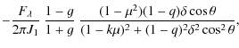
We begin with the known expression for the Faraday rotation
angle ![]() at the
Thomson optical path
at the
Thomson optical path ![]() that is frequently used below:
that is frequently used below:
where
Here
Silant'ev (2002)
derived the asymptotical
analytical formulae for the Stokes parameters of the radiation
emitted from a magnetized, optically thick, plane-parallel
atmosphere. For the Milne problem they are
where
![\begin{figure}
\par\includegraphics[width=7.8cm,clip]{10892_f1.eps}
\end{figure}](/articles/aa/full_html/2009/43/aa10892-08/img53.png)
|
Figure 1:
Main notions of accretion
disk surface, geometry of magnetic field |
| Open with DEXTER | |
Formulae (3, 4) for polarization consider the last
scattering
of radiation before escaping from a semi-infinite magnetized
atmosphere.
For a high value of parameter ![]() ,
the contribution of the secondary
scattered photons is small because of the large Faraday depolarization.
Even
in the absence of a magnetic field, the main contribution to the
polarization
of emitted radiation comes from the last scattered photons. For this
reason,
Eqs. (3), (4) at the absence of magnetic field
practically represent
the classical Chandrasekhar-Sobolev polarization in the Milne problem
(see, for example, Chandrasekhar 1950).
,
the contribution of the secondary
scattered photons is small because of the large Faraday depolarization.
Even
in the absence of a magnetic field, the main contribution to the
polarization
of emitted radiation comes from the last scattered photons. For this
reason,
Eqs. (3), (4) at the absence of magnetic field
practically represent
the classical Chandrasekhar-Sobolev polarization in the Milne problem
(see, for example, Chandrasekhar 1950).
As far as the intensity
of radiation ![]() is concerned, one can remember (see Chandrasekhar 1950)
that
the polarization weakly influences the intensity. For Milne's problem
without
the true absorption (q=0), we have
is concerned, one can remember (see Chandrasekhar 1950)
that
the polarization weakly influences the intensity. For Milne's problem
without
the true absorption (q=0), we have ![]() ,
whereas the separate
transfer equation with the Rayleigh phase function gives
,
whereas the separate
transfer equation with the Rayleigh phase function gives ![]() .
For high
values of
.
For high
values of ![]() ,
the terms with Stokes parameters Q
and U in the full system
of transfer equations for parameters I, Q
and U become very small
,
the terms with Stokes parameters Q
and U in the full system
of transfer equations for parameters I, Q
and U become very small ![]()
![]() ,
and they are negligible in the equation for intensity I.
As a result,
the radiation intensity obeys the separate transfer
equation with the Rayleigh phase function (see, Silant'ev 1994 for
more detail).
Expression (3) presents the solution to this equation. For
large
,
and they are negligible in the equation for intensity I.
As a result,
the radiation intensity obeys the separate transfer
equation with the Rayleigh phase function (see, Silant'ev 1994 for
more detail).
Expression (3) presents the solution to this equation. For
large ![]() the
main contribution to polarization comes from to intensity term.
Formulae (4) were
obtained in this way.
the
main contribution to polarization comes from to intensity term.
Formulae (4) were
obtained in this way.
Equations (2)-(4) allow us to derive the following approximate
expressions for polarization degree ![]() and
the position angle
and
the position angle ![]() of radiation for an accreting magnetized disk:
of radiation for an accreting magnetized disk:
where
The existence of a magnetic field, hence Faraday rotation,
only increases the depolarization process. It means that the
polarization of outgoing radiation acquires a peak-like angular
dependence with its maximum for perpendicular propagation. The
sharpness of the peak increases with increasing magnetic field
magnitude. The main region of allowed angles appears to be ![]()
![]() .
.
Another very important feature of the polarized
radiation is the wavelength dependence of polarization degree pand
position angle ![]() which is very different from
the case of classical electron
scattering. This effect is briefly considered in Sect. 5.
We consider the case where the Thomson
cross-section does not depend on the radiation wavelength.
which is very different from
the case of classical electron
scattering. This effect is briefly considered in Sect. 5.
We consider the case where the Thomson
cross-section does not depend on the radiation wavelength.
2.1 Integral polarization from the accretion disk
The axially symmetric accretion disks frequently are observed
as
a whole. The observed integral Stokes parameters ![]() and
and ![]() are described by the azimuthally averaged
formulae (3) and (4). To derive these expressions we introduce
the
following notions:
are described by the azimuthally averaged
formulae (3) and (4). To derive these expressions we introduce
the
following notions:
where
Using the axial symmetry of an accretion disk, we obtain (remember that

The observed degree of the light polarization and the position angle are derived from parameters (8) in the usual way. For particular cases of pure normal (
For perpendicular magnetic field are there the formulae
For a pure perpendicular magnetic field, the position angle
It is seen from Eqs. (8) that the
relative degree of polarization ![]() and position angle
and position angle ![]() only
depend on
dimensionless parameters a and b,
which are the functions of wavelength
only
depend on
dimensionless parameters a and b,
which are the functions of wavelength ![]() ,
magnetic fields
,
magnetic fields ![]() or
or ![]() ,
and inclination angle i (
,
and inclination angle i (
![]() ).
First we discuss the behavior of the relative degree of polarization
and
position angle on these two parameters. Remember that we consider
conservative atmosphere with
q=0, hence k=0. It is
interesting to investigate how the
polarization changes if we include the perpendicular magnetic field
).
First we discuss the behavior of the relative degree of polarization
and
position angle on these two parameters. Remember that we consider
conservative atmosphere with
q=0, hence k=0. It is
interesting to investigate how the
polarization changes if we include the perpendicular magnetic field ![]() in the
existing parallel magnetic field
in the
existing parallel magnetic field ![]() .
.
The average process takes the disk regions with the very
different angles ![]() into account between the magnetic field
into account between the magnetic field ![]() and the
line of sight
and the
line of sight ![]() ,
and the integral polarization and position
angle can acquire very different values. The numerical calculations
show that position angle
,
and the integral polarization and position
angle can acquire very different values. The numerical calculations
show that position angle ![]() not only depends on parameter
not only depends on parameter
![]() but also on the b - parameter
(
but also on the b - parameter
(
![]() ).
The existence of perpendicular magnetic
field
).
The existence of perpendicular magnetic
field ![]() diminishes the value of
diminishes the value of ![]() compared to the case
of pure parallel magnetic field. This decrease is especially large if b>aand
the parameters a and b
are close to unity. For
compared to the case
of pure parallel magnetic field. This decrease is especially large if b>aand
the parameters a and b
are close to unity. For ![]() and
b<a the decrease of
and
b<a the decrease of ![]() is small and practically
is small and practically ![]() .
But for
.
But for ![]() ,
the position angle
,
the position angle ![]() .
The
special case is
.
The
special case is ![]() .
In this case the position angle
.
In this case the position angle ![]() rapidly decreases from the
limiting value
rapidly decreases from the
limiting value ![]() for
for
![]() to value
to value ![]() at b=a, and then tends to zero
for
at b=a, and then tends to zero
for ![]() ,
so for large a the intermediate values of
,
so for large a the intermediate values of ![]() can only
occur in a rather narrow interval
can only
occur in a rather narrow interval ![]() ,
i.e. at
,
i.e. at
![]() .
.
The degree of linear polarization p depends on
parameters a and bin a
more complex form.
For ![]() the addition of the perpendicular magnetic
field (parameter b) lowers the integral
polarization. For a>1there is the region of b
(b<a) where the
polarization increases
compared with the case of pure parallel magnetic field. The maximum
polarization occurs at
the addition of the perpendicular magnetic
field (parameter b) lowers the integral
polarization. For a>1there is the region of b
(b<a) where the
polarization increases
compared with the case of pure parallel magnetic field. The maximum
polarization occurs at ![]() ,
and then the polarization decreases with
the increase in parameter b. The increase in
polarization at b=a can
be rather large. As a result, for value a=b=5,10,20,
and 50 the relative polarization
increase, as compared to purely parallel magnetic field, is equal to
160%, 224%,
317%, and 504%, respectively.
It seems this effect stems some ``resonant'' regions in
an accretion disk where the Faraday rotation from parallel magnetic
field
is balanced by opposite rotation from a perpendicular magnetic field.
Of course,
the magnitude of polarization decreases with the increase in a
and b.
The numerical calculations demonstrate that the relative polarization
degree
,
and then the polarization decreases with
the increase in parameter b. The increase in
polarization at b=a can
be rather large. As a result, for value a=b=5,10,20,
and 50 the relative polarization
increase, as compared to purely parallel magnetic field, is equal to
160%, 224%,
317%, and 504%, respectively.
It seems this effect stems some ``resonant'' regions in
an accretion disk where the Faraday rotation from parallel magnetic
field
is balanced by opposite rotation from a perpendicular magnetic field.
Of course,
the magnitude of polarization decreases with the increase in a
and b.
The numerical calculations demonstrate that the relative polarization
degree
![]() is a symmetric function of parameters aand b.
The position angle
is a symmetric function of parameters aand b.
The position angle ![]() does not possess this symmetry.
does not possess this symmetry.
Now we shortly discuss the wavelength dependence of polarization degree
![]() and
and ![]() ,
which follows from general formulae (8). More detailed
discussion is
presented in Sect. 5. For high values
of parameters a and (or) b the
spectra diminish
,
which follows from general formulae (8). More detailed
discussion is
presented in Sect. 5. For high values
of parameters a and (or) b the
spectra diminish ![]()
![]() .
But for the case a=b mentioned
above, the spectra diminish as
.
But for the case a=b mentioned
above, the spectra diminish as ![]()
![]() .
Thus, the ``resonant'' effect also changes the asymptotic behavior of
spectra.
Note once more that this effect disappears beyond the interval
.
Thus, the ``resonant'' effect also changes the asymptotic behavior of
spectra.
Note once more that this effect disappears beyond the interval ![]() .
The spectra
.
The spectra ![]() depend strongly on the relative value of
the perpendicular magnetic field
depend strongly on the relative value of
the perpendicular magnetic field ![]() as compared to vertical
component
as compared to vertical
component ![]() .
If parameter
.
If parameter ![]() and
and ![]() the position angle
the position angle ![]() ;
i.e., it becomes independent of wavelength. For the ``resonant'' case a=b,
this limiting value
is equal to
;
i.e., it becomes independent of wavelength. For the ``resonant'' case a=b,
this limiting value
is equal to ![]() .
.
The characteristic spectra of polarization and position
angle as a function of inclination angle i and
magnetic fields ![]() and
and
![]() are
presented in Fig. 2
(
are
presented in Fig. 2
(
![]() ). The mentioned case a=b
corresponds
to
). The mentioned case a=b
corresponds
to ![]() ;
i.e., at
;
i.e., at ![]() it exists at
it exists at
![]() .
For every
.
For every ![]() there exists its own value
there exists its own value
![]() ,
so, for
,
so, for ![]() m and
m and ![]() G,
this value is
a=b=2.828.
In this figure we present the relative polarization degree
G,
this value is
a=b=2.828.
In this figure we present the relative polarization degree
![]() for
the inclination angles
for
the inclination angles ![]() ,
and
,
and
![]() .
The values of the polarization degree
.
The values of the polarization degree
![]() for these
angles are equal to
for these
angles are equal to ![]() ,
2.25%, 1.08%,
and
,
2.25%, 1.08%,
and ![]() ,
respectively (see Chandrasekhar 1950).
The presented
spectra can help readers recognize general tendencies of polarization
as a function of the basic system parameters.
,
respectively (see Chandrasekhar 1950).
The presented
spectra can help readers recognize general tendencies of polarization
as a function of the basic system parameters.
![\begin{figure}
\par\includegraphics[width=14.5cm,clip]{10892_f2.eps}
\end{figure}](/articles/aa/full_html/2009/43/aa10892-08/img131.png)
|
Figure 2:
Spectra of relative
polarization degree |
| Open with DEXTER | |
We see that the
higher magnetic field, the larger depolarization. For
![]() and pure parallel magnetic field (
and pure parallel magnetic field (
![]() ),
the polarization degree tends to the Thomson value of polarization
),
the polarization degree tends to the Thomson value of polarization ![]() .
This is quite natural because in these cases the magnetic field is
practically perpendicular to the line of sight
.
This is quite natural because in these cases the magnetic field is
practically perpendicular to the line of sight ![]() ,
and the Faraday
rotation is low. The position angle
,
and the Faraday
rotation is low. The position angle ![]() is more sensitive to Faraday
rotation, and tends to Thomson value (
is more sensitive to Faraday
rotation, and tends to Thomson value (![]() )
slower than the polarization
degree tends to the Thomson polarization. It is interesting that for
this case
the relative polarization degrees
)
slower than the polarization
degree tends to the Thomson polarization. It is interesting that for
this case
the relative polarization degrees ![]() and
position angles
and
position angles ![]() practically coincide
for inclination angles
practically coincide
for inclination angles ![]() and
and ![]() ,
if the
magnetic fields differ 10 times (for example,
,
if the
magnetic fields differ 10 times (for example, ![]() and 50, or
and 50, or
![]() and
100, etc.). This happens because the corresponding values
of
and
100, etc.). This happens because the corresponding values
of ![]() ,
0.08715 and 0.86602, differ approximately 10 times.
,
0.08715 and 0.86602, differ approximately 10 times.
Comparing formulae (9) with (10), we find that the relative
polarization
degrees for perpendicular magnetic field (![]() can be taken from
the results drawn in Fig. 2a, if one uses
the substitution
can be taken from
the results drawn in Fig. 2a, if one uses
the substitution
![]() there. The case
there. The case ![]() G and
G and ![]() therefore
coincides with the case
therefore
coincides with the case ![]() G and
G and ![]() .
Of course, the
position angle
.
Of course, the
position angle ![]() for perpendicular magnetic field.
for perpendicular magnetic field.
For the case ![]() (see Fig. 2b)
the most depolarization
occurs at
(see Fig. 2b)
the most depolarization
occurs at ![]() ,
in contrast to the pure parallel
magnetic field. It is interesting that the
relative degrees of polarization are the same for the inclinations
i and
,
in contrast to the pure parallel
magnetic field. It is interesting that the
relative degrees of polarization are the same for the inclinations
i and ![]() .
But the position angles are different in these
cases. The relative polarization degree is higher for
.
But the position angles are different in these
cases. The relative polarization degree is higher for ![]() than for
than for ![]() ,
i.e. the change in this value is not monotonic.
The case
,
i.e. the change in this value is not monotonic.
The case ![]() corresponds to equality
corresponds to equality ![]() .
As
mentioned above, in this case
.
As
mentioned above, in this case ![]() .
The righthand side
of Fig. 2b
confirms this.
.
The righthand side
of Fig. 2b
confirms this.
Figure 2c
presents the spectra of the relative polarization degree and position
angle for ![]() G
and
G
and ![]() G (the curves
denoted by the usual
numbers) and the opposite case
G (the curves
denoted by the usual
numbers) and the opposite case ![]() G and
G and ![]() G
(the curves
denoted by numbers in brackets). The symmetry of
relative polarization degree as a function of parameters a
and b gives rise
to the coincidence of spectra in the first case with those in the
second case if
the angle
G
(the curves
denoted by numbers in brackets). The symmetry of
relative polarization degree as a function of parameters a
and b gives rise
to the coincidence of spectra in the first case with those in the
second case if
the angle ![]() ,
so the relative polarization degree spectra
at
,
so the relative polarization degree spectra
at ![]() and
and
![]() coincide with
the spectra denoted as
coincide with
the spectra denoted as ![]() and
and
![]() ,
respectively. But the position-angle spectra are different for
these two cases.
,
respectively. But the position-angle spectra are different for
these two cases.
The spectra, presented in Fig. 2, demonstrate a large variability of values and forms for polarization degrees and position angles in the integral radiation escaping from the magnetized accretion disks.
2.2 Some results from accretion disk models
Models of a magnetic accretion disk with externally imposed, large- scale vertical magnetic field and anomalous magnetic field diffusion due to enhanced turbulent diffusion have been considered by Campbell (2000), Ogilvie & Livio (2001), and Pariev et al. (2003).
We calculate the value of Faraday depolarization parameter
![]() for the model
of an accreting disk suggesting the
power-law radial dependence of the magnetic field:
for the model
of an accreting disk suggesting the
power-law radial dependence of the magnetic field:
where B(r) is the magnetic field inside an accretion disk, and
where
Pariev et al. (2003) have
developed the detailed description of magnetized
accretion disks with the different values for parameter n
(denoted as ![]() in
their paper). The radial effective temperature dependence
in
their paper). The radial effective temperature dependence ![]() in
their model is the same as in the Shakura-Sunyaev model. They find
that, in the case
of equipartition of magnetic pressure with radiation or thermal
pressures, their
results are close to Shakura-Sunyaev model with the viscosity parameter
in
their model is the same as in the Shakura-Sunyaev model. They find
that, in the case
of equipartition of magnetic pressure with radiation or thermal
pressures, their
results are close to Shakura-Sunyaev model with the viscosity parameter
![]() .
As a most
physically significant model, they investigate the case n=5/4
in more detail.
Parameter n must be greater than unity if we
consider the disks
with the diminishing gas density far from the black hole. It should
also be noted
that dependence (11) with n=5/4 takes place at the
equipartition of magnetic
energy with thermal and gravitational ones in the spherical accretion
(see, for
example, Melia 1992).
Following to Pariev et al. (2003), we
use mostly
the case n=5/4.
.
As a most
physically significant model, they investigate the case n=5/4
in more detail.
Parameter n must be greater than unity if we
consider the disks
with the diminishing gas density far from the black hole. It should
also be noted
that dependence (11) with n=5/4 takes place at the
equipartition of magnetic
energy with thermal and gravitational ones in the spherical accretion
(see, for
example, Melia 1992).
Following to Pariev et al. (2003), we
use mostly
the case n=5/4.
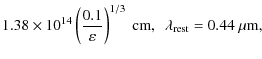
The central problem is to derive the characteristic scale
![]() that corresponds to the effective wavelength of
polarimetric observations. At first glance, we can estimate the
radius
that corresponds to the effective wavelength of
polarimetric observations. At first glance, we can estimate the
radius ![]() ,
suggesting that
,
suggesting that ![]() corresponds
to the value of rest-frame wavelength of the black body
spectrum maximum,
corresponds
to the value of rest-frame wavelength of the black body
spectrum maximum,
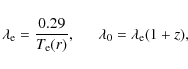
where
In a standard thin disk model (Shakura &
Sunyaev 1973),
there are a black body radiation with an effective
temperature profile of ![]() and the scale
length
and the scale
length ![]() defined by the point in the disk where the disk temperature
matches the rest-frame wavelength of the monitoring band.
defined by the point in the disk where the disk temperature
matches the rest-frame wavelength of the monitoring band.
There is the series of papers where the semi-empirical method of
determining of the accretion disk scale ![]() has been developed (see
Kochanek et al. 2006;
Poindexter et al. 2008;
Morgan et al. 2007, 2008).
The authors used microlensing variability observed for
gravitationally lensed quasars to find the accretion disk size and
the observed (or rest-frame) wavelength relation. It is very
important that the scaling appeared to be consistent with what is
expected from the thin accretion disk theory of Shakura &
Sunyaev (1973).
has been developed (see
Kochanek et al. 2006;
Poindexter et al. 2008;
Morgan et al. 2007, 2008).
The authors used microlensing variability observed for
gravitationally lensed quasars to find the accretion disk size and
the observed (or rest-frame) wavelength relation. It is very
important that the scaling appeared to be consistent with what is
expected from the thin accretion disk theory of Shakura &
Sunyaev (1973).
This allows us to have the following size scaling (Poindexter
et al.
2008):
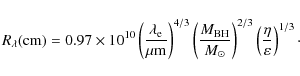
Here

Theoretical calculations of parameter
The strong gravitational field near the black hole influences the Stokes parameters of outgoing radiation when they propagate to an observer. The detailed calculations of this effect have been done by Connors et al. (1980), Karas et al. (2004), and Dovciak et al. (2004). Usually these effects are important when describing X-ray emission from the vicinity of the black hole. The optical radiation arises far from this place, and we neglect these gravitational corrections.
3 Magnetic field strength of NGC 4258
NGC 4258 is a low-luminosity Seyfert II
galaxy at the distance of
about 7.2 Mpc, which harbors water masers (Modjaz
et al.
2005).
This object is usually considered as a very good
laboratory for successfully measuring the magnetic field in accretion
disk
even very close to the central black hole.
The spatial velocity distribution of water mega-maser sources in
NGC 4258 on scales of 0.14-0.28 pc indicates a thin
Keplerian disk
rotating around a black hole with a mass ![]() (Herrnstein et al. 1999).
The
accretion disk has an almost edge-on orientation with the
radiation axis and its inclination angle is
(Herrnstein et al. 1999).
The
accretion disk has an almost edge-on orientation with the
radiation axis and its inclination angle is ![]() (Pringle et al. 1999). A
pc-scale jet closely
aligns in projection on the sky with the rotation axis (Herrnstein
et al. 1997).
(Pringle et al. 1999). A
pc-scale jet closely
aligns in projection on the sky with the rotation axis (Herrnstein
et al. 1997).
Modjaz et al. (2005)
present an analysis of polarimetric
observations at 22 GHz of the water vapor masers in
NGC 4258
obtained with the VLA and the GBT. They do not detect any
circular polarization in the spectrum indicative of Zeeman-induced
splitting of the maser lines of water, and obtained only an upper
limit on the magnetic field strengths. They obtained the
1-![]() upper
limit value of the toroidal component of the
magnetic field at a radius of 0.2 pc the value of
90 mG and
determined a 1-
upper
limit value of the toroidal component of the
magnetic field at a radius of 0.2 pc the value of
90 mG and
determined a 1-![]() upper limit of 30 mG on the radial
component at a radius of 0.14 pc. They also find from their
observations
of magnetic field limits that the geometrically thin disk model and the
jet-disk model are better candidates for accounting for the extremely
low-luminosity of NGC 4258.
upper limit of 30 mG on the radial
component at a radius of 0.14 pc. They also find from their
observations
of magnetic field limits that the geometrically thin disk model and the
jet-disk model are better candidates for accounting for the extremely
low-luminosity of NGC 4258.
More recently, Reynolds et al. (2008)
have shown from analysis of
SUZAKU and XMM-Newton observational data that the observed iron lines
originate in the surface layers of an warped accretion disk at
the distance ![]() from the black hole.
In contrast to the majority of Seifert 2 galaxies, there was
no
indication of a Compton-thick obscuring torus. The weak iron line and
the lack of a reflection point to circumnuclear environment that is
remarkably clean of cold gas. They note that such a circumnuclear
environment
is only found in two AGNs - NGC 4258 and M81 that contrast to
the
majority of Seifert 2 galaxies.
from the black hole.
In contrast to the majority of Seifert 2 galaxies, there was
no
indication of a Compton-thick obscuring torus. The weak iron line and
the lack of a reflection point to circumnuclear environment that is
remarkably clean of cold gas. They note that such a circumnuclear
environment
is only found in two AGNs - NGC 4258 and M81 that contrast to
the
majority of Seifert 2 galaxies.
This picture coincides with one by Herrnstein et al. (2005)
pointed out earlier. According to them the observing intrinsic
absorption in the X-ray spectrum can arise in
the outer layers of the warped geometrically-thin accretion disk at the
distance ![]() 29 pc
from the black hole, where the molecular-to-atomic transition occurs.
29 pc
from the black hole, where the molecular-to-atomic transition occurs.
This picture allowed us to use our simple model of arising of optical polarized radiation without taking the warp contribution into account. Of course, the power-law dependence of the magnetic field is an important assumption in our derivation. This assumption is now commonly accepted (see Pariev et al. 2003).
The detected of polarized continuum and line emission from the
nucleus of NGC 4258 was by Wilkes et al.
(1995).
After that, Barth et al. (1999)
obtained spectropolarimetric observations of the NGC 4258
nucleus
at the Keck II telescope. The observations were obtained on
1997
April 10 UT at the Keck II telescope with
the LRIS
spectropolarimeter. The results of these observations are
presented in the Table 1
of the paper by Barth et al.
(1999).
For the continuum polarization they obtained the
following results:
We see that the polarization is weakly increasing to the short wavelength range, but the value of a position angle is practically constant. The position angles
3.1 Estimates of magnetic field in the model of nonturbulent accretion disk
For the inclination angle ![]() ,
the
expected polarization should have the value
,
the
expected polarization should have the value ![]() .
From Eqs. (9) and (10)
for degree of polarization
we find that possible parameters
.
From Eqs. (9) and (10)
for degree of polarization
we find that possible parameters ![]() and
and
![]() are near the value 20. The
position angle
are near the value 20. The
position angle ![]() for this value of a is equal to
for this value of a is equal to ![]() ,
which is far from observing values (see Eq. (21)). From the
discussion
in Sect. 2.1 we know that for high values of parameters a
and b,
the possibility of small position angles exists if
,
which is far from observing values (see Eq. (21)). From the
discussion
in Sect. 2.1 we know that for high values of parameters a
and b,
the possibility of small position angles exists if ![]() .
.
The exact formulae (8) give us the values
a=122 and b=122.9, which
correspond to observed values of
polarization degree 0.38% and ![]() at
at ![]() m.
These values correspond to
m.
These values correspond to ![]() (or
(or ![]() G ) and
G ) and
![]() (or
(or ![]() G). The analogous
values of
parameters for the polarization degree 0.35% and
G). The analogous
values of
parameters for the polarization degree 0.35% and ![]() at
at
![]() m are
m are ![]() (or
(or ![]() G) and
G) and
![]() (or
(or ![]() G).
For the case
G).
For the case
![]() m (
m (
![]() ),
the formulae (8)
give
),
the formulae (8)
give ![]() G
and
G
and ![]() G.
We see that in all cases
the normal magnetic field
G.
We see that in all cases
the normal magnetic field ![]() is greater than
is greater than ![]() .
Because
the effective temperature
.
Because
the effective temperature ![]() decreases with the increase in the
distance from the inner radius of an accretion disk, we conclude that
magnetic field also decreases with the growing distance.
decreases with the increase in the
distance from the inner radius of an accretion disk, we conclude that
magnetic field also decreases with the growing distance.
What seems unsatisfactory in these results is their
sensitivity to small variations in parameters a and
b. If these
parameters change their values (
![]() )
slightly the
solution is impossible. For magnetic fields it means that the values
have not to change its values greater than 10 G. This is very
improbable for real situations in accretion disks. For this reason
we have to seek a more satisfactory model where this sensitivity does
not
occur. Such a model really exists. It takes into account that the
magnetic
field can be turbulent.
)
slightly the
solution is impossible. For magnetic fields it means that the values
have not to change its values greater than 10 G. This is very
improbable for real situations in accretion disks. For this reason
we have to seek a more satisfactory model where this sensitivity does
not
occur. Such a model really exists. It takes into account that the
magnetic
field can be turbulent.
3.2 Estimates of magnetic field in the model of turbulent accretion disk
According to Silant'ev (2005, 2007) the
chaotic
component ![]() of the magnetic field (
of the magnetic field (
![]() ),
where
),
where ![]() is a regular part of the magnetic field,
gives rise to additional extinction of the intensity of linearly
polarized
waves (parameters Q and U) due
to small scale chaotic Faraday rotations.
The Gaussian distribution of turbulent velocities was assumed.
Mathematically,
this effect is analogous to the known problem of diffusion of scalar
impurity
in a stochastic velocity field (see, for example, van Kampen 1981). In
our case,
the Faraday rotation angle replaces the role of impurity.
The main part of the effective cross-section
is a regular part of the magnetic field,
gives rise to additional extinction of the intensity of linearly
polarized
waves (parameters Q and U) due
to small scale chaotic Faraday rotations.
The Gaussian distribution of turbulent velocities was assumed.
Mathematically,
this effect is analogous to the known problem of diffusion of scalar
impurity
in a stochastic velocity field (see, for example, van Kampen 1981). In
our case,
the Faraday rotation angle replaces the role of impurity.
The main part of the effective cross-section ![]() corresponding
to this additional extinction, takes a very simple form:
corresponding
to this additional extinction, takes a very simple form:
Here,
The asymptotic formulae taking this effect into account have
the same form
as formulae (3-5) with the substitution ![]() .
(Remember that we consider the conservative atmosphere with q=k=0.)
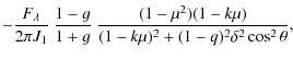
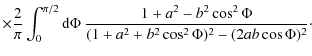
In particular, the formulae (8) acquire the form
.
(Remember that we consider the conservative atmosphere with q=k=0.)
In particular, the formulae (8) acquire the form
![$\displaystyle \quad\times\frac{2}{\pi}\int_{0}^{\pi/2}{\rm d}\Phi
\frac{(1+C)^2+a^2+b^2\cos^2\Phi}{[(1+C)^2+a^2+b^2\cos^2\Phi]^2
-(2ab\cos\Phi)^2}$](/articles/aa/full_html/2009/43/aa10892-08/img214.png)
![$\displaystyle \quad\times
\frac{2}{\pi}\int_{0}^{\pi/2}{\rm d}\Phi\frac{(1+C)^2+a^2-b^2\cos^2\Phi}{[(1+C)^2+a^2+b^2\cos^2\Phi]^2
-(2ab\cos\Phi)^2}\cdot$](/articles/aa/full_html/2009/43/aa10892-08/img216.png)
Here parameters a and b are presented by formulae (7), where
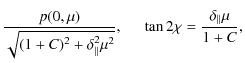
The parameter C is fairly large for our
case, ![]() .
In this
case the term
.
In this
case the term ![]() in denominators of formulae (18) can be
neglected and we obtain the following analytical expressions:
in denominators of formulae (18) can be
neglected and we obtain the following analytical expressions:
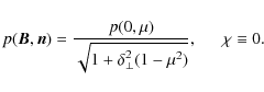
![$\displaystyle \frac{p(0,\mu)}{[(1+C)^2+a^2]\sqrt{(1+d)}}
\sqrt{(1+C)^2+\frac{a^2}{(1+d)^2}}\cdot$](/articles/aa/full_html/2009/43/aa10892-08/img223.png)
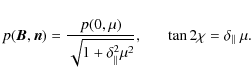
These expressions are fairly exact up to a,b<C. If parameters a or bare equal to zero, formulae (19) are exact. In particular, for the cases of pure normal regular magnetic field
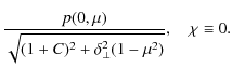
In the limit case of nonturbulent magnetic field (C=0), they coincide with the formulae (9) and (10). If the chaotic magnetic field B' is fairly high (
The existence of
new parameter C describing the level of magnetic
field fluctuations
makes the estimation of mean values of ![]() and
and ![]() difficult.
In our case this problem is simpler because the level of magnetic
fluctuations (parameter C) changes slowly with the
variations in parameters
a and b. Indeed, for the pure
normal magnetic field (b=0) we found
a=7.37,
C=15.5 for
difficult.
In our case this problem is simpler because the level of magnetic
fluctuations (parameter C) changes slowly with the
variations in parameters
a and b. Indeed, for the pure
normal magnetic field (b=0) we found
a=7.37,
C=15.5 for ![]() m;
a=4.77, C=18.13
for
m;
a=4.77, C=18.13
for
![]() ,
and a=6.56,
C=21.88 at
,
and a=6.56,
C=21.88 at ![]() .
In the limiting case of high values of polarization degree (a=b),
these
values are: a=b=8,
C=14; a=b=5,
C=17.5, and a=b=7,
C=21,
respectively; i.e., parameter C is practically the
same for these two cases.
.
In the limiting case of high values of polarization degree (a=b),
these
values are: a=b=8,
C=14; a=b=5,
C=17.5, and a=b=7,
C=21,
respectively; i.e., parameter C is practically the
same for these two cases.
For this reason we calculate the a and b
parameters using the mean
values for parameter C; i.e., C=14.75,
17.81 and 21.44, respectively.
This gives the values a=8, b=6
(
![]() G) for
G) for ![]() m; for
m; for ![]() m - a=5,
b=3.5 (
m - a=5,
b=3.5 (
![]() G);
and for
G);
and for ![]() m - a=7,
b=5.5(
m - a=7,
b=5.5(
![]() G).
These values of magnetic fields are lowere
than those for the case of nonturbulent accretion disk. But important
is that
they were derived without restriction
G).
These values of magnetic fields are lowere
than those for the case of nonturbulent accretion disk. But important
is that
they were derived without restriction ![]() .
.
Let us estimate the
level of magnetic fluctuations taking the mean values for parameter C.
We also assume that fB=1
and ![]() .
We do not know the real distribution
of turbulent eddies in a turbulent accretion disk. The general picture
of turbulence
consists of cascade of eddies with different dimensions. The small
eddies with
.
We do not know the real distribution
of turbulent eddies in a turbulent accretion disk. The general picture
of turbulence
consists of cascade of eddies with different dimensions. The small
eddies with ![]() includes a value propto a parameter C.
The large
eddies do not allow us to describe the considered effect in the range
of radiative
transfer equations. It seems that our value
includes a value propto a parameter C.
The large
eddies do not allow us to describe the considered effect in the range
of radiative
transfer equations. It seems that our value ![]() is fairly natural for
describing the turbulent effects in magnetized plasma. If we increase
is fairly natural for
describing the turbulent effects in magnetized plasma. If we increase ![]() to k-times,
then the level of magnetic fluctuations
to k-times,
then the level of magnetic fluctuations ![]() decreases to k-times.
The real value of parameter
decreases to k-times.
The real value of parameter ![]() can therefore be estimated by independent estimation of
magnetic fluctuations.
After that we obtain the values
can therefore be estimated by independent estimation of
magnetic fluctuations.
After that we obtain the values
![]() G,
and 49 G for the mean square root values of magnetic
fluctuations at places where the thermal radiation
has a maximum for
G,
and 49 G for the mean square root values of magnetic
fluctuations at places where the thermal radiation
has a maximum for ![]() ,
and
,
and ![]() ,
respectively. These values of fluctuations are equal to 31%, 56%, and
44% of
the mean magnetic fields for mentioned wavelengths.
,
respectively. These values of fluctuations are equal to 31%, 56%, and
44% of
the mean magnetic fields for mentioned wavelengths.
3.3 Estimates of the magnetic field at the horizon of the black hole in NGC 4258
We now proceed to the estimation of the magnetic field strength in NGC 4258 using the maser polarimetric data. The magnetic field structures in accretion disks are difficult to observe and remain poorly known. If the disk is penetrated by a dipole field of the central object or by a global field of the surrounding interstellar medium, there may be a net vertical flux. Sano et al. (2004) consider the models of an accretion disk with a uniform magnetic field. The stress forces in accretion disks may be proportional to Bz (Hawley et al. 1995) or to Bz2 (Turner et al. 2003).
Zhang & Dai (2008) have studied the effect of a global magnetic field on viscously rotating and vertically integrated accretion disks around compact objects using a self-similar treatment. They show that the strong magnetic field in the vertical direction prevents the disk from being accreted and decreases the effect of the gas pressure.
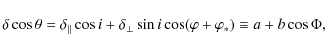
On the other hand, Königl (1989) and Cao (1997)
underline that the inclination of the field lines at the surface
of the disk plays a crucial role in the magnetically
driven outflow. They show that, for the nonrelativistic case, a
centrifugally driven outflow of matter from the disk is only
possible if the poloidal component of the magnetic field makes an
angle less than a critical ![]() with the disk surface.
with the disk surface.
Now let us estimate the value of ![]() for the model of a
standard accretion disk using the observational data of
NGC 4258.
The spatial structure of standard accretion disk have been
calculated by Poindexter et al. (2008).
The size
scaling is determined by Eq. (14). The basic physical
parameters of the central nucleus of NGC 4258 are
for the model of a
standard accretion disk using the observational data of
NGC 4258.
The spatial structure of standard accretion disk have been
calculated by Poindexter et al. (2008).
The size
scaling is determined by Eq. (14). The basic physical
parameters of the central nucleus of NGC 4258 are ![]() and
and ![]() (Satyapal et al. 2005).
We use these
estimations below in numerical calculations.
(Satyapal et al. 2005).
We use these
estimations below in numerical calculations.
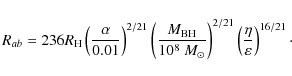
The estimates of the scaleradius ![]() from
Eq. (14) give the following results:
from
Eq. (14) give the following results:
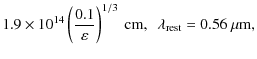
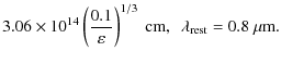
For
The formulae (21) for arbitrary wavelength
These estimates show that
This means that the characteristic spatial radius of an accretion disk
We use the polarimetric data by Modjaz et al. (2005).
These data allow a ![]() upper limit of
upper limit of ![]() mG
on the radial component of the disk magnetic field at the
radius of 0.14 pc. Using the power-law radial dependence of
magnetic field (11), we obtain the following expression:
mG
on the radial component of the disk magnetic field at the
radius of 0.14 pc. Using the power-law radial dependence of
magnetic field (11), we obtain the following expression:
where
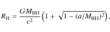
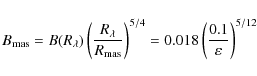
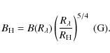
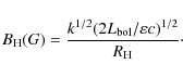
Finally, we can estimate the magnetic field strength ![]() at the
horizon radius of the black hole in NGC 4258 using the data
for
at the
horizon radius of the black hole in NGC 4258 using the data
for ![]() presented in expressions (22),
and for our values
presented in expressions (22),
and for our values ![]() for the
turbulent accretion disk model (see Sect. 3.2).
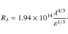
Taking in Eq. (11)
for the
turbulent accretion disk model (see Sect. 3.2).
Taking in Eq. (11) ![]() ,
we obtain the expression:
,
we obtain the expression:
As a result, we obtain for
Our estimates are
slightly different as a result of different error intervals of
polarimetric data (see Eq. (16)). Besides, some
uncertainty exists in the choice of the level of fluctuations
(parameter C).
It seems for ![]() m that this
uncertainty is less than for other
wavelengths. For this reason the estimate
m that this
uncertainty is less than for other
wavelengths. For this reason the estimate ![]() G
seems to be
preferable. As an example, we present the estimates for this effective
wavelength and other various
parameters
G
seems to be
preferable. As an example, we present the estimates for this effective
wavelength and other various
parameters ![]() and
and ![]() in Table 1.
in Table 1.
In the estimations, presented above we take n=5/4
in the basic Eq. (11).
How do we change the estimations for other values of n?
The calculations give
the following values of ![]() at the event horizon of the supermassive black
hole in NGC 4258:
at the event horizon of the supermassive black
hole in NGC 4258: ![]() G
at n=1, and
G
at n=1, and ![]() G
at
n=2. These results indicate that the magnetic field
strength of SMBH in
NGC 4258 at the event horizon should be at the level
G
at
n=2. These results indicate that the magnetic field
strength of SMBH in
NGC 4258 at the event horizon should be at the level ![]() 103-104 G.
103-104 G.
It should be noted that our estimations do not use the values of
viscosity parameter ![]() .
It was only shown that, for
.
It was only shown that, for ![]() ,
the radius
,
the radius
![]() lies inside zone (a). Of course, our estimations depend
on parameters
lies inside zone (a). Of course, our estimations depend
on parameters ![]() and the power-law index n, which, in
principle,
are to be found in a detailed model of an accretion disk.
and the power-law index n, which, in
principle,
are to be found in a detailed model of an accretion disk.
The data in Pariev et al. (2003) are
given for ![]() (
(
![]() is the gravitational radius of black hole),
i. e. slightly beyond the horizon radius
is the gravitational radius of black hole),
i. e. slightly beyond the horizon radius ![]() (beyond
(beyond ![]() for
for ![]() ,
and beyond
,
and beyond ![]() for
for ![]() ). It seems
that they used the simplified
theory, which do not ``work'' near the horizon. The calculations in
Pariev et al. (2003)
correspond to magnetic dominated regime; i.e., magnetic energy is
greater than
radiative thermal energy. Because
). It seems
that they used the simplified
theory, which do not ``work'' near the horizon. The calculations in
Pariev et al. (2003)
correspond to magnetic dominated regime; i.e., magnetic energy is
greater than
radiative thermal energy. Because ![]() lies inside the zone (a) (radiation
dominated zone), we derive that plasma parameter
lies inside the zone (a) (radiation
dominated zone), we derive that plasma parameter ![]() in model of
Pariev et al. (2003).
Here
in model of
Pariev et al. (2003).
Here ![]() and
and ![]() are gas and magnetic pressures,
respectively.
are gas and magnetic pressures,
respectively.
Table
1:
The value of ![]() [G]
for various data of Kerr parameter
and radiative efficiency.
[G]
for various data of Kerr parameter
and radiative efficiency.
4 Magnetic coupling process in AGN and QSO: testing by continuum polarization
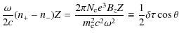
Li (2002), Wang et al. (2002, 2003), Zhang et al. (2005) studied the magnetic coupling process (MC) as an effective mechanism for transferring energy and angular momentum from a rotating black hole to its surrounding accretion disk. This process can be considered as one of the variants of the Blandford-Znajek (BZ) process (Blandford & Znajek 1977; Blandford & Payne 1982). It is assumed that the disk is stable, perfectly conducting, thin, and Keplerian. The magnetic field is assumed to be constant on the black hole horizon and to vary as a power law with the radius of the accretion disk.
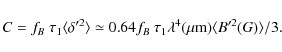
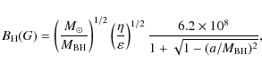
Since the magnetic field on the horizon ![]() is brought and held
by its surrounding magnetized matter of a disk,
the some relation must exist between the magnetic field strength and
accretion disk and, finally, the bolometric luminosity
of AGN (see Ma et al. 2007). This
relation takes a form
is brought and held
by its surrounding magnetized matter of a disk,
the some relation must exist between the magnetic field strength and
accretion disk and, finally, the bolometric luminosity
of AGN (see Ma et al. 2007). This
relation takes a form
Here
Then Eq. (27) is transformed into
where
We next calculate the expected polarization value of radiation
in a
number of specific AGNs, taking the effect of Faraday
depolarization into account, as considered above. In mechanisms of
magnetic coupling,
we mainly consider the case where magnetic field is supposed directed
along the normal to the accretion disk (see, for example,
Wang et al. 2002;
Ma et al. 2007).
Our estimates of the magnetic field in NGC 4258 (see
Sect. 3.2) show that the vertical magnetic field is much
larger than the perpendicular one.
For these reasons, we also consider only ![]() fields as
first approximation, so we have to determine
fields as
first approximation, so we have to determine
![]() from Eq. (25). The values
from Eq. (25). The values ![]() and
and ![]() are presented
in Eqs. (12) and (14), and
are presented
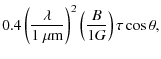
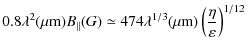
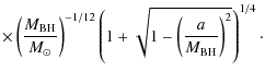
in Eqs. (12) and (14), and ![]() - in Eq. (28). As a result, we obtain the
following formula for dimensionless parameter
- in Eq. (28). As a result, we obtain the
following formula for dimensionless parameter ![]() :
:
The estimations of polarization degree
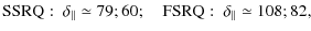
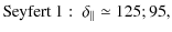
A systematic analysis of a large sample of AGN
available in the BeppoSAX public archive was performed by
Grandi et al. (2006).
Their sample includes AGN of
various types. Narrow line radio galaxies (NLRG), broad line radio
galaxies (BLRG), steep spectrum radio quasars (SSRQ) and flat
spectrum radio quasars (FSRQ) (see Table 6 from their paper,
where
the values ![]() and
and ![]() are presented.
are presented.
The results of our calculations of the dimensionless
depolarization parameter ![]() are
are
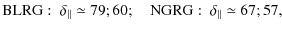
where the first numbers correspond to
The estimations of possible ![]() for the inclination angle of the
accretion disk
for the inclination angle of the
accretion disk ![]() (
(
![]() )
are presented in Table 2.
Because all values of
)
are presented in Table 2.
Because all values of ![]() ,
we can use the approximate formula
,
we can use the approximate formula
![]() .
This formula is valid up to
.
This formula is valid up to ![]() ,
so for
,
so for ![]() (
(
![]() )
the polarization degree
is to 20 times higher than values presented in Table 2
(
)
the polarization degree
is to 20 times higher than values presented in Table 2
(
![]() ).
For other inclination angles
i, the calculations are analogous. We stress that
polarization observations of sources,
presented in Table 2,
do not exist up to now, so we present only possible values of
polarization degrees. This procedure, presented below, can be used to
estimate
the source parameters if the polarization data are available.
).
For other inclination angles
i, the calculations are analogous. We stress that
polarization observations of sources,
presented in Table 2,
do not exist up to now, so we present only possible values of
polarization degrees. This procedure, presented below, can be used to
estimate
the source parameters if the polarization data are available.
The limiting case ![]() corresponds to
corresponds to ![]() ;
i.e.,
the predicted polarizations differ only slightly from the
presented values for
;
i.e.,
the predicted polarizations differ only slightly from the
presented values for ![]() ,
so for the source NGC 4258 instead
of
,
so for the source NGC 4258 instead
of ![]() G, corresponding to
G, corresponding to ![]() (see Table 1),
we obtain
(see Table 1),
we obtain ![]() G
for limiting case
G
for limiting case ![]() .
.
Table 2: The value of linear polarization from accretion disks.
5 The wavelength dependence of polarization of AGN and accretion disk models
Polarization in AGNs can be intrinsic or extrinsic. Light scattering by a nonspherical distribution of electrons near the central engine of AGN is a basic intrinsic polarization mechanism; namely, an accretion disk is a typical example of a nonspherical distribution. Scattering by magnetically aligned dust grains in the interstellar medium of galaxies is the typical example of an extrinsic situation. The very important feature characterizing the polarized radiation from a magnetized accretion disk is the wavelength dependence of polarization degree that is very different from that of Thomson's scattering.
For a strong magnetic field strength, when ![]() the simple asymptotic formulas follow from
Eqs. (9) and (10):
the simple asymptotic formulas follow from
Eqs. (9) and (10):
For turbulent atmospheres, with the existence of chaotic magnetic field component B', the corresponding asymptotic formulae follow from Eqs. (20). If the parameter of turbulence
The wavelength dependencies of the radiation flux and its
polarization essentially stem from the radial distribution of the
temperature in an accretion disk. For a standard accretion disk
(Shakura & Sunyaev 1973),
radial dependence of the temperature takes
the form: ![]() .
To get the integrated spectrum from the disk,
we add up all of the Planck curves from each radius. If
.
To get the integrated spectrum from the disk,
we add up all of the Planck curves from each radius. If ![]() then
the radiation flux (see Pringle & Rees 1972;
Shakura & Syunyaev 1973;
Gaskell 2008):
then
the radiation flux (see Pringle & Rees 1972;
Shakura & Syunyaev 1973;
Gaskell 2008):

For a standard accretion disk (s=3/4), the flux (30) takes the known form
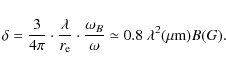
Substitution of ![]() into
formula (13) leads to relation
into
formula (13) leads to relation ![]() between
the characteristic scale
between
the characteristic scale ![]() and the effective wavelength of
polarimetric observations. According to
expression (11) we obtain
and the effective wavelength of
polarimetric observations. According to
expression (11) we obtain ![]() .
As a result, from Eqs. (31) and (11), we obtain the
next wavelength
dependence for the case of a strong Faraday depolarization:
.
As a result, from Eqs. (31) and (11), we obtain the
next wavelength
dependence for the case of a strong Faraday depolarization:
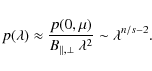
As a result, the degree of observed polarization
For distribution of magnetic field in a standard
accretion disk (s=3/4) with n=3/2
(
![]() ),
the polarization does not depend on the wavelength. For a standard
accretion disk
with n=5/4, mostly elaborated by Pariev
et al. (2003),
the wavelength dependence
of the polarization is quite weak
),
the polarization does not depend on the wavelength. For a standard
accretion disk
with n=5/4, mostly elaborated by Pariev
et al. (2003),
the wavelength dependence
of the polarization is quite weak ![]() .
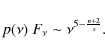
In this case
the wavelength dependence of the Stokes polarized flux takes the
form
.
In this case
the wavelength dependence of the Stokes polarized flux takes the
form ![]() .
In the general case the formulae (32) and (33) give
rise to relation
.
In the general case the formulae (32) and (33) give
rise to relation
The presented formulas allow us to test the various models of an accretion disk using the data of the wavelength dependence of polarization of AGN and quasars.
For the turbulent accretion disk with a high value of
parameter C,
formula (34) transforms to the expression
The position angle values
5.1 Discussion of some observational data
Webb et al. (1993)
and Impey et al. (1995)
present the data
of measurement UBVRI polarizations
of a sample of AGNs and QSOs.
The position angle appears to be wavelength-independent,
suggesting that the polarization in a given object originates in a
single physical process. In many cases the percentage of
polarization increases with frequency. Authors have compared the
polarized fluxes with the predictions of competing models of
polarization in AGNs: synchrotron emission, scattering from
electrons or different types of dust grains, and electron
scattering in an accretion flow. In nine sources from this sample,
the polarization seems to be the result of dust grain
scattering. A number of these sources (NGC 4151,
Mrk 509,
NGC 5548, Mrk 290) has best characteristics of model
due to
electron
scattering in an accretion disk or torus. It is interesting that,
for these four sources, the slopes of
![]() are
close (
are
close (
![]() ,
-0.9, -0.86, -0.9, respectively;
see Webb et al. (1993).
According to formula (32), we obtain the
corresponding values of parameter s=0.46,
0.47, 0.52, 0.51; i.e.,
they are near s=0.5.
,
-0.9, -0.86, -0.9, respectively;
see Webb et al. (1993).
According to formula (32), we obtain the
corresponding values of parameter s=0.46,
0.47, 0.52, 0.51; i.e.,
they are near s=0.5.
The general shape of the polarization spectrum with
parameter ``q'' was determined by a
least-squares fit proportional to
![]() .
It appears that the slope of the
wavelength dependence of polarized flux q varies
widely, between -2 and +1, with a typical uncertainty
of 0.3.
.
It appears that the slope of the
wavelength dependence of polarized flux q varies
widely, between -2 and +1, with a typical uncertainty
of 0.3.
What values of parameter n corresponds to limit
values of
q, if we accept s=1/2 using
formulas (34) and (35)?
For nonturbulent accretion disk (Eq. (34)) we obtain

This formula gives n=1.5 for q=-2, n=1 for q=-1, n=0.5 for q=0, and n=0 for q=1. Remember (see Pariev et al. 2003) that accretion disk with decreasing gas density at large distances r corresponds to n>1. It seems the self-consistent models of Pariev et al. (2003) allow the values of
For this reason we investigate what gives the very high
magnetic turbulence.
For this case, formula (32) transforms to expression ![]() .
It leads to
.
It leads to ![]() at s=1/2. As a result, our physically
acceptable restriction 1<n<2 allows
us, in principle, to explain the decreasing
degree of polarization. Taking the definition
at s=1/2. As a result, our physically
acceptable restriction 1<n<2 allows
us, in principle, to explain the decreasing
degree of polarization. Taking the definition ![]() into account,
we derive from Eq. (34) the following relation
into account,
we derive from Eq. (34) the following relation
For s = 0.5 this expression gives n = 1 for q = 1, and n=1.5 for q=0. For q = -2 this formula gives n = 5/2, which characterizes a very sharp decrease in magnetic field inside the accretion disk.
As an example, we now consider the continuum radiation of
source NGC 4151. According
to Webb et al. (1993),
we have ![]() ,
and from Schmidt & Miller (1980)
the parameter q is equal to
,
and from Schmidt & Miller (1980)
the parameter q is equal to ![]() (see Fig. 3 for the
value
(see Fig. 3 for the
value ![]() in the interval
in the interval ![]() m).
From Eq. (31) we obtain
m).
From Eq. (31) we obtain ![]() ,
which gives in
this case
,
which gives in
this case ![]() .
Substitution of the values q=-0.33 and s=0.46
to Eq. (37)
gives
.
Substitution of the values q=-0.33 and s=0.46
to Eq. (37)
gives ![]() .
In nonturbulent case we have
.
In nonturbulent case we have ![]() ,
which
corresponds to the increase in gas density with growing distance from
the
nucleus (see Pariev et al. 2003). In
our case, when we know the observed spectra
,
which
corresponds to the increase in gas density with growing distance from
the
nucleus (see Pariev et al. 2003). In
our case, when we know the observed spectra ![]() ,
and
,
and
![]() ,
both Eqs. (34) and (35) give rise to the same
expression
,
both Eqs. (34) and (35) give rise to the same
expression ![]() .
Thompson
et al. (1979,
see Fig. 3) present the polarization degree
.
Thompson
et al. (1979,
see Fig. 3) present the polarization degree ![]() in the same
interval
in the same
interval ![]() m.
The data have a rather wide distribution.
Using our dependence, we can approximate the polarization degree
by the formula
m.
The data have a rather wide distribution.
Using our dependence, we can approximate the polarization degree
by the formula ![]() m),
which fairly satisfactorily describes the mean value of the presented
data.
m),
which fairly satisfactorily describes the mean value of the presented
data.
6 Conclusions
We have presented the method for estimating the magnetic field strength at the event horizon of a supermassive black hole through the polarization of accreting disk emission. The polarized radiation arises from the scattering of emission light by electrons in a magnetized accretion disk. Due to Faraday rotation of the polarization plane, the resulting polarization degree differs essentially from the classical Thomson case, because the wavelength dependence of the polarization degree appears. This feature means that the magnetic field strength at the event horizon of a black hole can be estimated from polarimetric observations in the optical range.
For estimating observed polarization, we use the azimuthally averaged asymptotic expressions of the Stokes parameters for outgoing radiation, assuming that the accretion disk is optically thick and that the Milne problem takes place. Using these formulae, we discuss the wavelength dependence of the observed spectra of polarization degree. We also consider turbulent accretion disks when the magnetic field possess both regular component and chaotic one. Since the polarization spectrum of scattered radiation strongly depends on the accretion disk model, our results can be used to construct a realistic physical model of the AGN environment.
The estimates of the magnetic field strength of
supermassive black holes in NGC 4258 are presented. We also
found for the source
NGC 4151 that the observed polarization degree spectrum can be
satisfactorily
explained by our mechanism with the high level of turbulent magnetic
field. In this case the power-law regular magnetic field is ![]() and
and ![]() .
In the cases where the observed polarization is the result of various
mechanisms,
such as light scattering in an accretion disk and a jet, our method can
be considered
as important part of the problem as a whole.
.
In the cases where the observed polarization is the result of various
mechanisms,
such as light scattering in an accretion disk and a jet, our method can
be considered
as important part of the problem as a whole.
This research was supported by the RFBR (project No. 07-02-00535a), the program of Prezidium of RAS ``Origin and Evolution of Stars and Galaxies'', the program of the Department of Physical Sciences of RAS ``Extended Objects in the Universe'' and by the Grant from President of the Russian Federation ``The Basic Scientific Schools'' NS-6110.2008.2. M.Yu. Piotrovich acknowledges the Council of Grants of the President of the Russian Federation for Young Scientists, grant No. 4101.2008.2.We are very grateful to the anonymous referee for many remarks that allowed us to clarify the paper considerably.
References
- Agol, E., & Blaes, O. 1996, MNRAS, 282, 965 [NASA ADS]
- Barth, A. J., Tran, H. D., Brotherton, M. S., et al. 1999, AJ, 118, 1609 [CrossRef] [NASA ADS]
- Blaes, O. 2003, in Accretion discs, jets and high energy phenomena in astrophysics, Les Houches Session LXXXIII, 2002, ed. V. Beskin et al. (N.Y.: Springer)
- Blandford, R. D., & Payne, D. C. 1982, MNRAS, 199, 883 [NASA ADS]
- Blandford, R. D., & Znajek, R. L. 1977, MNRAS, 179, 433 [NASA ADS]
- Campbell, C. G. 2000, MNRAS, 317, 501 [CrossRef] [NASA ADS]
- Cao, X. 1997, MNRAS, 291, 145 [NASA ADS]
- Chandrasekhar, S. 1950, Radiative transfer (Oxford: Clarendon press)
- Chang, P., Quataert, E., & Murray, N. 2007, ApJ, 662, 94 [CrossRef] [NASA ADS]
- Connors, P. A., Piran, T., & Stark, R. F. 1980, ApJ, 235, 224 [CrossRef] [NASA ADS]
- Dolginov, A. Z., Gnedin, Yu. N., & Silan'ev, N. A. 1995, Propagation and polarization of radiation in cosmic media (N.Y.: Gordon & Breach)
- Dovciak, M., Karas, V., & Matt, G. 2004, MNRAS, 355, 1005 [CrossRef] [NASA ADS]
- Gaskell, C. M. 2008, Rev. Mex. Astron. Astrophys. (serie de Conferencias), 32, 1 [NASA ADS]
- Gnedin, Yu. N., & Silant'ev, N. A. 1997, Basic Mechanisms of Light Polarization in Cosmic Media (Amsterdam: Hartwood)
- Gnedin, Yu. N., Silant'ev, N. A., & Shternin, P. S. 2006, Astron. Lett., 32, 39 [CrossRef] [NASA ADS]
- Grandi, P., Malaguti, G., & Fiocchi, M. 2006, ApJ, 642, 113 [CrossRef] [NASA ADS] [arXiv:astro-ph/0511784]
- Hawley, J. F., Gammie, C. F., & Balbus, S. A. 1995, ApJ, 440, 742 [CrossRef] [NASA ADS]
- Herrnstein, J. R., Moran, J. M., Greenhill, L. J., et al. 1997, ApJ, 475, L17 [CrossRef] [NASA ADS]
- Herrnstein, J. R., Moran, J. M., Greenhill, L. J., et al. 1999, Nature, 400, 539 [CrossRef] [NASA ADS]
- Herrnstein, J. R., Moran, J. M., Greenhill, L. J., & Trotter, A. S. 2005, ApJ, 629, 719 [CrossRef] [NASA ADS]
- Impey, C. D., Malkan, M. A., Webb, W., & Petry, C. E. 1995, ApJ, 440, 80 [CrossRef] [NASA ADS]
- Karas, V., Dovciak, M., & Matt, G. 2004, 22th Texas Symposium on relativistiv astrophysics at Stanford University
- Kochanek, C. S., Dai, X., Morgan, C., Morgan, N. & Poindexter, S. 2006 [arXiv:astro-ph/0609112]
- Königl, A. 1989, ApJ, 342, 208 [CrossRef] [NASA ADS]
- Krolik, J. H. 2007 [arXiv:0709.1489]
- Kroll, N. A., & Trivelpiece, A. W. 1973, Principles of plasma physics (N.Y.: McCraw-Hill)
- Li, L. X. 2002, A&A, 392, 469 [EDP Sciences] [CrossRef] [NASA ADS]
- Ma, R.-Y., Yang, F., & Wang, D.-X. 2007, ApJ, 671, 1981 [CrossRef] [NASA ADS]
- Martin, P. G. 1989, IAUS, 135, 55 [NASA ADS]
- Martin, P. G., Thompson, I. B., Maza, J., & Angel, J. R. P. 1983, ApJ, 266, 470 [CrossRef] [NASA ADS]
- Melia, F. 1992, ApJ, 387, L25 [CrossRef] [NASA ADS]
- Modjaz, M., Moran, J. M., Kondratko, P. T., & Greenhill, L. J. 2005, ApJ, 626, 104 [CrossRef] [NASA ADS]
- Moran, J. 2008, ASPC, 395, 87 [NASA ADS]
- Morgan, C., Kochanek, C. S., Morgan, N. D. & Falco, E. E. 2006, ApJ, 647, 874 [CrossRef] [NASA ADS]
- Morgan, C. W., Kochanek, C. S., Dai, X., Morgan, N. D., & Falco, E. E. 2008, ApJ, 689, 755 [CrossRef] [NASA ADS]
- Novikov, I. D., & Thorne, K. 1973, Black Holes, ed. C. De Witt-Morette, & B. C. De Witt (New York: Gordon and Breach)
- Ogilvie, G. I., & Livio, M. 2001, ApJ, 553, 158 [CrossRef] [NASA ADS]
- Pariev, V. I., Blackman, E. G., & Boldyrev, S. A. 2003, A&A, 407, 403 [EDP Sciences] [CrossRef] [NASA ADS]
- Pariev, V. I., & Colgate, S. A. 2007, ApJ, 658, 129 [CrossRef] [NASA ADS]
- Poindexter, S., Morgan, N., & Kochanek, C. 2008, ApJ, 673, 34 [CrossRef] [NASA ADS]
- Pringle, J. E., & Rees, M. J. 1972, A&A, 21, 1 [NASA ADS]
- Pringle, J. E., Antonucci, R. R. J., Clarke, C. J., et al. 1999, ApJ, 526, L9 [CrossRef] [NASA ADS]
- Reynolds, S. R., Nowak, M. A., Markoff, S., et al. 2008 [arXiv:0810.2543]
- Rohlfs, K., & Wilson, T. L. 1996, Tools of Radio Astronomy (Berlin: Springer)
- Satyapal, S., Dudik, R. P., O'Halloran, B., & Gliozzi, M. 2005, ApJ, 633, 865 [CrossRef]
- Sano, T., Inutsiko, S.-I., Turner, N. J., & Stone, J. M. 2004, ApJ, 605, 321 [CrossRef] [NASA ADS]
- Schmidt, G. D., & Miller, J. S. 1980, ApJ, 240, 759 [CrossRef] [NASA ADS]
- Serkowskii, K. 1973, IAUS, 52, 145 [NASA ADS]
- Shakura, N. I., & Sunyaev, R. A. 1973, A&A, 24, 337 [NASA ADS]
- Shapiro, S. 2007 [arXiv:0711.1537]
- Shternin, P. S., Gnedin, Yu. N., & Silant'ev, N. A. 2003, Astrofizika, 46, 433
- Silant'ev, N. A. 1994, JQSRT, 52, 207 [NASA ADS]
- Silant'ev, N. A. 2002, A&A, 383, 326 [EDP Sciences] [CrossRef] [NASA ADS]
- Silant'ev, N. A. 2005, A&A, 433, 1117 [EDP Sciences] [CrossRef] [NASA ADS]
- Silant'ev, N. A. 2007, Astron. Rep., 51, 67 [CrossRef] [NASA ADS]
- Smith, J. E., Young, S., Robinson, A., et al. 2002, MNRAS, 355, 773 [CrossRef] [NASA ADS]
- Thompson, I., Landstreet, J. D., Angel, J. R. P., et al. 1979, ApJ, 229, 909 [CrossRef] [NASA ADS]
- Turner, N. J., Stone, J. M., Krolik, J. H., & Sano, T. 2003, ApJ, 593, 992 [CrossRef] [NASA ADS]
- van Kampen, N. G. 1981, Stochastic processes in Physics and Chemistry (Amsterdam: North Holland)
- Webb, W., Malkan, M., Schmidt, G., & Impey, C. 1993, ApJ, 419, 494 [CrossRef] [NASA ADS]
- Wang, D.-X., Xiao, K. & Lei, W.-H. 2002, MNRAS, 335, 655 [CrossRef] [NASA ADS]
- Wang, D.-X., Ma, R.-Y., Lei, W.-H., & Yao, G.-Z. 2003, ApJ, 595, 109 [CrossRef] [NASA ADS]
- Wilkes, B. J., Schmidt, G. D., Smith, P. S., et al. 1995, ApJ, 455, L13 [CrossRef] [NASA ADS]
- Zhang, D., & Dai, Z. G. 2008, MNRAS, 388, 1409 [CrossRef] [NASA ADS]
- Zhang, W. M., Lu, Y., & Zhang, S. N. 2005, Chin. J. Astron. Astrophys. , 5, Suppl., 347
All Tables
Table
1: The value of ![]() [G] for various data
of Kerr parameter
and radiative efficiency.
[G] for various data
of Kerr parameter
and radiative efficiency.
Table 2: The value of linear polarization from accretion disks.
Current usage metrics show cumulative count of Article Views (full-text article views including HTML views, PDF and ePub downloads, according to the available data) and Abstracts Views on Vision4Press platform.
Data correspond to usage on the plateform after 2015. The current usage metrics is available 48-96 hours after online publication and is updated daily on week days.
Initial download of the metrics may take a while.