| Issue |
A&A
Volume 506, Number 3, November II 2009
|
|
|---|---|---|
| Page(s) | 1123 - 1135 | |
| Section | Extragalactic astronomy | |
| DOI | https://doi.org/10.1051/0004-6361/200911698 | |
| Published online | 27 August 2009 | |
A&A 506, 1123-1135 (2009)
Cosmic rays and the magnetic field in the nearby starburst galaxy NGC 253
II. The magnetic field structure![[*]](/icons/foot_motif.png)
V. Heesen1,3 - M. Krause2 - R. Beck2 - R.-J. Dettmar3
1 - Centre for Astrophysics Research, University of Hertfordshire, Hatfield AL10 9AB, UK
2 - Max-Planck-Institut für Radioastronomie, Auf dem Hügel 69, 53121 Bonn, Germany
3 - Astronomisches Institut der Ruhr-Universität Bochum, Universitätsstr. 150, 44780 Bochum, Germany
Received 21 January 2009 / Accepted 29 July 2009
Abstract
Context. There are several edge-on galaxies with a known
magnetic field structure in their halo. A vertical magnetic field
significantly enhances the cosmic-ray transport from the disk into the
halo. This could explain the existence of the observed radio halos.
Aims. We observed NGC 253 that possesses one of the
brightest radio halos discovered so far. Since this galaxy is not
exactly edge-on (
![]() )
the disk magnetic field has to be modeled and subtracted from the
observations in order to study the magnetic field in the halo.
)
the disk magnetic field has to be modeled and subtracted from the
observations in order to study the magnetic field in the halo.
Methods. We used radio continuum polarimetry with the VLA in
D-configuration and the Effelsberg 100-m telescope. NGC 253 has a
very bright nuclear point-like source, so that we had to correct for
instrumental polarization. We used appropriate Effelsberg beam patterns
and developed a tailored polarization calibration to cope with the
off-axis location of the nucleus in the VLA primary beams. Observations
at
![]() 6.2 cm and 3.6 cm were combined to calculate the RM distribution and to correct for Faraday rotation.
6.2 cm and 3.6 cm were combined to calculate the RM distribution and to correct for Faraday rotation.
Results. The large-scale magnetic field consists of a disk ![]() and a halo (r,z) component. The disk component can be described as an axisymmetric spiral field pointing inwards with a pitch angle of
and a halo (r,z) component. The disk component can be described as an axisymmetric spiral field pointing inwards with a pitch angle of
![]() which is symmetric
with respect to the plane (even parity). This field dominates in the
disk, so that the observed magnetic field orientation is disk parallel
at small distances from the midplane. The halo field shows a prominent
X-shape centered on the nucleus similar to that of other edge-on
galaxies. We propose a model where the halo field lines are along a
cone with an opening angle of
which is symmetric
with respect to the plane (even parity). This field dominates in the
disk, so that the observed magnetic field orientation is disk parallel
at small distances from the midplane. The halo field shows a prominent
X-shape centered on the nucleus similar to that of other edge-on
galaxies. We propose a model where the halo field lines are along a
cone with an opening angle of
![]() and are pointing away from the disk in both the northern and southern
halo (even parity). We can not exclude that the field points inwards in
the northern halo (odd parity). The X-shaped halo field follows the
lobes seen in H
and are pointing away from the disk in both the northern and southern
halo (even parity). We can not exclude that the field points inwards in
the northern halo (odd parity). The X-shaped halo field follows the
lobes seen in H![]() and soft X-ray emission.
and soft X-ray emission.
Conclusions. Dynamo action and a disk wind can explain the
X-shaped halo field. The nuclear starburst-driven superwind may further
amplify and align the halo field by compression of the lobes of the
expanding superbubbles. The disk wind is a promising candidate for the
origin of the gas in the halo and for the expulsion of small-scale
helical fields as requested for efficient dynamo action.
Key words: galaxies: individual: NGC 253 - magnetic fields - methods: observational - methods: data analysis - galaxies: halos - galaxies: ISM
1 Introduction
There is increasing observational evidence for the existence of gaseous halos around disk galaxies. They consist of different interstellar medium (ISM) species, mainly the diffuse ionized gas, dust, cosmic rays (CRs), and magnetic fields (for a review, see e.g. Dettmar 1992). The transport of gas from the disk into the halo has been discussed in the past in terms of galactic chimneys (Norman & Ikeuchi 1989) and superbubble blow outs (Mac Low & Ferrara 1999). These models all include supernova explosions as the energy source that drives the formation of the halo. The effects of star formation on the ISM are dramatic: the heated gas in supernova remnants and accelerated energetic particles are injected into the base of the halo. The fundamental parameter, which determines the formation of a halo, is therefore the energy input by supernova explosions. Thus, the halo does not form above the entire disk, but only at radial distances where the star formation takes place (Dahlem et al. 1995). Moreover, the compactness of the star-forming regions determines the threshold condition where the hot gas can break out against the pull of the gravitational field (Dahlem et al. 2006). This corroborates the picture of the hot gas injected by supernova explosions and stellar winds of massive stars (see e.g. Dettmar & Soida 2006).
Direct evidence for supernova-heated galactic halos comes from imaging and spectroscopy of diffuse soft X-ray emission. This has been impressively demonstrated by XMM-Newton observations of NGC 253 where the nuclear X-ray plume can be explained only by star formation without the contribution of an AGN (Bauer et al. 2008; Pietsch et al. 2001). Moreover, it clearly shows that the galactic starburst must drive a thermal outflow, since there are strong indications of collisionally excited oxygen and iron L line complexes in the spectrum (Breitschwerdt 2003).
In a pioneering work Ipavich (1975) pointed out the importance of CRs for the generation of a galactic wind. In the disk, the CR gas, the magnetic field, and the hot gas contribute roughly the same amount of pressure (Beck et al. 1996). In the halo, however, CRs and the magnetic field dominate. The relativistic CR gas has a larger pressure scaleheight than the hot gas, because its adiabatic index is 4/3whereas it is 5/3 for the hot gas; the magnetic field has an even larger scaleheight (Beck 2007). Furthermore, the CR nucleons, which contain the bulk of the energy, do not suffer from strong radiative losses like the hot gas. The CR-driven galactic wind is thus another scenario which needs consideration when discussing gaseous halos.
The theoretical framework for the CR transport is given by the combined diffusion-convection equation, which can be applied in the local comoving coordinate system if the bulk speed of the background medium is non-relativistic (Schlickeiser 2002). Breitschwerdt et al. (1993,1991) applied the transport equation for different magnetic field configurations in the Milky Way. They concluded that the CR transport can be split in an entirely diffusive and an entirely convective regime, depending only on the local magnetic field configuration. For the lower Milky Way halo they assumed the magnetic field lines to be turbulently excited by stochastic gas motions caused by expanding and overlapping supernova remnants. Thus, there will be no preferred direction of propagation of these magnetic fluctuations and hence no net Alfvénic drift. In the halo the magnetic field lines of the superbubbles begin to overlap and form ``open'' field lines that might be enhanced by magnetic reconnection (Parker 1992).
Various polarization studies have shown that magnetic fields are a very
sensitive tracer of interaction in the ISM that is not visible at any other
wavelength. Chyzy & Beck (2004) showed that the interacting pair of galaxies
NGC 4038/39 (the Antennae) possesses a strong magnetic field of
![]() ,
significantly stronger than non-interacting spirals. The polarized
emission in many of the Virgo cluster galaxies is shifted with respect to the
optical distribution (Wezgowiec et al. 2007). Simulations suggest that this
behavior can be explained by ram pressure stripping of galaxies moving through
the intracluster medium (Vollmer et al. 2008; Soida et al. 2006). But a close inspection
of the Virgo spiral NGC 4254 showed that the observed magnetic field
structure requires additional MHD mechanisms other than ram pressure stripping
(Chyzy 2008; Chyzy et al. 2007). The structure of the magnetic field is thus an
important tracer for MHD processes and the interaction between various ISM
components, which are expected to be present in galaxies with winds.
,
significantly stronger than non-interacting spirals. The polarized
emission in many of the Virgo cluster galaxies is shifted with respect to the
optical distribution (Wezgowiec et al. 2007). Simulations suggest that this
behavior can be explained by ram pressure stripping of galaxies moving through
the intracluster medium (Vollmer et al. 2008; Soida et al. 2006). But a close inspection
of the Virgo spiral NGC 4254 showed that the observed magnetic field
structure requires additional MHD mechanisms other than ram pressure stripping
(Chyzy 2008; Chyzy et al. 2007). The structure of the magnetic field is thus an
important tracer for MHD processes and the interaction between various ISM
components, which are expected to be present in galaxies with winds.
From these considerations it is clear that there is a need for understanding
the three-dimensional structure of the magnetic field in the halo of spiral
galaxies. That restricts the observations to a few nearby edge-on galaxies
that allow us to study the extra-planar magnetic field with high spatial
resolution and sensitivity. Several edge-on galaxies have a known magnetic
field structure (Golla & Hummel 1994; Krause 2009; Tüllmann et al. 2000; Dettmar & Soida 2006; Krause 2004; Dumke & Krause 1998). The nearby starburst galaxy NGC 253 possesses
one of the brightest radio halos discovered so far, but the inclination angle
is only mildly edge-on (
![]() ). We assumed a distance of 3.94 Mpc (Karachentsev et al. 2003) where an angular resolution of
). We assumed a distance of 3.94 Mpc (Karachentsev et al. 2003) where an angular resolution of
![]() corresponds to a spatial resolution of 600 pc. Furthermore, we used
corresponds to a spatial resolution of 600 pc. Furthermore, we used
![]() as the position angle of the major axis.
as the position angle of the major axis.
This paper is the successive paper of Heesen et al. (2009) (Paper I thereafter) where the CR distribution in NGC 253 was found to be consistent with a vertical CR transport from the disk into the halo. In contradiction to this finding so far no vertical magnetic field has been discovered in the halo of this galaxy. The most detailed discussion of the magnetic field structure was presented by Beck et al. (1994), where a mainly disk-parallel magnetic field was found in the disk and halo. This was explained by a strong shearing of the magnetic field due to differential rotation. The study presented in the present paper provides new sensitive observations of the large-scale magnetic field in the halo of NGC 253. We use the polarimetry information of the observations presented in Paper I at different wavelengths which allow us to apply a correction for the Faraday rotation and thus to determine the intrinsic magnetic field orientation.
This paper is organized as follows: we start with the description of the observations and explain especially the calibration of the polarization in order to cope with instrumental polarization caused by the high dynamic range (Sect. 2). We present the continuum maps of NGC 253 along with the vectors of the intrinsic magnetic field and briefly describe its morphology in Sect. 3. Section 4 summarizes the polarization properties. In Sect. 5 we investigate the magnetic field structure and present a model for the large-scale magnetic field. In Sect. 6 we discuss the consequences of our findings for the radio halo of NGC 253 and the observed other phases of the ISM. Finally we summarize our results and present the conclusions in Sect. 7.
2 Observations and data reduction
2.1 Effelsberg observations
In Paper I we described our radio continuum observations of NGC 253 at
![]()
![]() and
and
![]() with the 100-m Effelsberg
telescope
with the 100-m Effelsberg
telescope![]() . Here we only explain the
details important for the polarization measurements and for the general
calibration and data reduction we refer to Paper I. The high dynamic range
(
. Here we only explain the
details important for the polarization measurements and for the general
calibration and data reduction we refer to Paper I. The high dynamic range
(![]() 1000) due to the strong nuclear point-like source (hereafter for
simplicity called the nucleus) requires several additional steps in the data
reduction. In Paper I we explained how we removed the sidelobes of the nucleus
via a Högbom cleaning of the total power maps. But the high dynamic range
also influences the polarization via the leakage of total power emission to
the polarized intensity. The flux density of the so-called instrumental
polarization is about 1.0% for the Effelsberg telescope with respect
to the total power flux density (Heesen 2008). Thus, it can be neglected
only for observations with a dynamic range significantly less than 100 which
is not fulfilled for our observations.
1000) due to the strong nuclear point-like source (hereafter for
simplicity called the nucleus) requires several additional steps in the data
reduction. In Paper I we explained how we removed the sidelobes of the nucleus
via a Högbom cleaning of the total power maps. But the high dynamic range
also influences the polarization via the leakage of total power emission to
the polarized intensity. The flux density of the so-called instrumental
polarization is about 1.0% for the Effelsberg telescope with respect
to the total power flux density (Heesen 2008). Thus, it can be neglected
only for observations with a dynamic range significantly less than 100 which
is not fulfilled for our observations.
In order to apply a correction for the instrumental polarization we used beam
patterns for Stokes parameters Q and U obtained from deep observations of
the unpolarized point-like source 3C84. The cleaned total power emission was
convolved with the beam patterns and the computed instrumental contribution
was subtracted from the Stokes Q and U maps, respectively. Finally we
obtained the map of the polarized intensity from the corrected Stokes Q and
U maps using COMB (part of AIPS)![]() . We applied a correction for the noise bias in
order to preserve the mean zero level of the polarized intensity. The rms
noise levels of the final maps are
. We applied a correction for the noise bias in
order to preserve the mean zero level of the polarized intensity. The rms
noise levels of the final maps are
![]() for
for
![]() at
at
![]() resolution and
resolution and
![]() for
for
![]()
![]() at
at
![]() resolution, respectively
resolution, respectively![]() .
.
2.2 VLA observations
For the polarization calibration of the VLA mosaic at ![]()
![]() (see Paper I) we met the challenge that the nucleus is located at the edge of
the primary beam in some of our pointings
(see Paper I) we met the challenge that the nucleus is located at the edge of
the primary beam in some of our pointings![]() . In the
center of the primary beam the instrumental polarization is less than 0.1%
but at the edge of the primary beam it rises to more than 1%. The
variability in time due to the apparent circular motion of the nucleus around
the center in the primary beam, caused by the alt-azimuthal mount of the VLA
antennas, complicates the situation even further. This prevents the removal of
sidelobes with the Högbom clean algorithm as it works only for non-variable
sources. Thus, the standard polarization calibration technique applied in case
of NGC 253 leads to a polarization map completely dominated by instrumental
polarization.
. In the
center of the primary beam the instrumental polarization is less than 0.1%
but at the edge of the primary beam it rises to more than 1%. The
variability in time due to the apparent circular motion of the nucleus around
the center in the primary beam, caused by the alt-azimuthal mount of the VLA
antennas, complicates the situation even further. This prevents the removal of
sidelobes with the Högbom clean algorithm as it works only for non-variable
sources. Thus, the standard polarization calibration technique applied in case
of NGC 253 leads to a polarization map completely dominated by instrumental
polarization.
Hence, we developed a specially tailored technique for the pointings with the nucleus located at the edge of the primary beam. The polarization calibration PCAL (part of AIPS) was applied to the nucleus itself instead of the secondary (phase) calibrator in order to find a solution for the off-axis instrumental polarization. The appropriate beam patterns in Stokes Q and U allowed us to subtract the nucleus from the (u,v)-data of individual ``snapshots'', which contained less than 10 min of observing time. This effectively removes the time-variable contribution of the instrumental polarization caused by the nucleus. Thus we were able to use the full set of (u,v)-data in order to get the best (u,v)-coverage which resulted in the expected sensitivity of the extended emission. A more detailed description of the polarization calibration can be found in Heesen (2008).
The pointings that are not influenced by the nucleus were calibrated
in the standard way with the secondary calibrator using PCAL. Inverting the (u,v)-data with natural weighting (i.e. Briggs Robust = 8) we produced maps of all pointings in Stokes Q and U, which were convolved with a Gaussian to
![]() resolution. The
combination of the pointings was done with LTESS (part of AIPS) which
performs a linear superposition with a correction for the VLA primary
beam attenuation using information from each pointing out to the 7%
level of the primary beam (Braun 1988). The final maps are
essentially noise limited with a sensitivity of
resolution. The
combination of the pointings was done with LTESS (part of AIPS) which
performs a linear superposition with a correction for the VLA primary
beam attenuation using information from each pointing out to the 7%
level of the primary beam (Braun 1988). The final maps are
essentially noise limited with a sensitivity of
![]() at
at
![]() resolution in Stokes Q and U. We used IMERG (part
of AIPS) for the combination of the VLA and Effelsberg Stokes Q and
U maps in order to fill in the missing zero-spacing flux; this was
done for the total power (Stokes I) map also. The map of the
polarized intensity was computed again using POLC with a correction
for the noise bias.
resolution in Stokes Q and U. We used IMERG (part
of AIPS) for the combination of the VLA and Effelsberg Stokes Q and
U maps in order to fill in the missing zero-spacing flux; this was
done for the total power (Stokes I) map also. The map of the
polarized intensity was computed again using POLC with a correction
for the noise bias.
3 Morphology of the polarized emission
![\begin{figure}
\par\includegraphics[bb=45 180 570 640,width=8.5cm,clip]{11698fig1}
\end{figure}](/articles/aa/full_html/2009/42/aa11698-09/img46.png)
|
Figure 1:
Total power radio continuum at |
| Open with DEXTER | |
![\begin{figure}
\par\includegraphics[bb=15 70 530 530,width=8.5cm,clip]{11698fig2}
\end{figure}](/articles/aa/full_html/2009/42/aa11698-09/img49.png)
|
Figure 2:
Total power radio continuum at |
| Open with DEXTER | |
![\begin{figure}
\par\includegraphics[bb=45 180 570 640,width=8.5cm,clip]{11698fig3}
\end{figure}](/articles/aa/full_html/2009/42/aa11698-09/img55.png)
|
Figure 3:
Total power radio continuum at |
| Open with DEXTER | |
In Fig. 1 we present the
distribution of the total power radio continuum emission together with
the B-vectors from the ![]()
![]() Effelsberg
observations. The low resolution of
Effelsberg
observations. The low resolution of
![]() shows the magnetic
field structure at the largest scales. The magnetic field is
disk parallel only in the disk plane. Further away from the disk, it
has a significant vertical component.
shows the magnetic
field structure at the largest scales. The magnetic field is
disk parallel only in the disk plane. Further away from the disk, it
has a significant vertical component.
Table 1: Maps of NGC 253 presented in this paper of total power radio continuum (TP) and polarized intensity (PI).
From the combined VLA + Effelsberg observations atWe show the ![]()
![]() Effelsberg map in
Fig. 3. At a resolution of
Effelsberg map in
Fig. 3. At a resolution of
![]() this map reveals no new details. But it is important
for the determination of the Faraday rotation as shown in
Sect. 4.2.
this map reveals no new details. But it is important
for the determination of the Faraday rotation as shown in
Sect. 4.2.
The distribution of the polarized intensity from the ![]()
![]() Effelsberg observations is presented in
Fig. 4. It is very different from
the total power distribution that can be be described by a thick radio
disk with a vertical exponential
profile. Figure 4 shows a thick
disk formed by extensions E1 and E2, apparent in the VLA + Effelsberg map
(Fig. 5).
Effelsberg observations is presented in
Fig. 4. It is very different from
the total power distribution that can be be described by a thick radio
disk with a vertical exponential
profile. Figure 4 shows a thick
disk formed by extensions E1 and E2, apparent in the VLA + Effelsberg map
(Fig. 5).
Figure 5 shows the distribution of the
polarized intensity from the combined ![]()
![]() VLA +
Effelsberg observations. The bulk of the polarized emission arises in
the disk and extends into the halo. In contrast, in the outer parts of
the disk the polarized emission is weak at this resolution. The
polarized emission extends to large vertical heights above the inner
disk. The Effelsberg
VLA +
Effelsberg observations. The bulk of the polarized emission arises in
the disk and extends into the halo. In contrast, in the outer parts of
the disk the polarized emission is weak at this resolution. The
polarized emission extends to large vertical heights above the inner
disk. The Effelsberg ![]()
![]() map of the polarized
intensity presented in Fig. 6 is
similar to Fig. 5 where the emission
is slightly more concentrated to the disk than at
map of the polarized
intensity presented in Fig. 6 is
similar to Fig. 5 where the emission
is slightly more concentrated to the disk than at ![]()
![]() .
This can be explained by the smaller scaleheight of the total
power emission at this shorter wavelength due to higher synchrotron
losses that influences also the polarized emission (see Paper I).
.
This can be explained by the smaller scaleheight of the total
power emission at this shorter wavelength due to higher synchrotron
losses that influences also the polarized emission (see Paper I).
The polarized intensity has a minimum between the radio spur S1 and the extension E2. Another minimum of polarized intensity is located near the radio spur S2. We will refer to these regions as ``depolarized regions''. The large-scale magnetic field is disk parallel near the galactic midplane whereas at some locations we find a significant vertical component. Hence, the large-scale magnetic field may consist of two components, one disk parallel and one vertical.
![\begin{figure}
\par\includegraphics[bb=45 160 570 660,width=8.5cm,clip]{11698fig4}
\end{figure}](/articles/aa/full_html/2009/42/aa11698-09/img59.png)
|
Figure 4:
Polarized intensity at |
| Open with DEXTER | |
4 Polarization properties
4.1 Degree of polarization
Linearly polarized synchrotron emission is observed from CR electrons
spiraling in an ordered magnetic field. No linearly polarized signal is
detected from isotropic turbulent magnetic fields with randomly distributed
directions![]() . Hence, we can use the polarization degree as a
measure of the ratio between the ordered and the turbulent magnetic field.
. Hence, we can use the polarization degree as a
measure of the ratio between the ordered and the turbulent magnetic field.
The integrated polarized flux densities were obtained by integration in
ellipses which include the extra-planar emission as described in Paper I (see
Table 2). The error of the flux densities was calculated as
the quadratic sum of a 5% calibration error and the baselevel error. The
polarization degree P is the ratio of the flux density of the extended total
power emission ![]() (nucleus subtracted) to that of the polarized
emission
(nucleus subtracted) to that of the polarized
emission ![]() .
The polarization degree is between 6% and 9%,
which is similar to values found in other galaxies.
.
The polarization degree is between 6% and 9%,
which is similar to values found in other galaxies.
![\begin{figure}
\par\includegraphics[bb=10 60 530 520,width=8.5cm,clip]{11698fig5}
\end{figure}](/articles/aa/full_html/2009/42/aa11698-09/img63.png)
|
Figure 5:
Polarized intensity at |
| Open with DEXTER | |
![\begin{figure}
\par\includegraphics[bb=50 160 570 660,width=8.5cm,clip]{11698fig6}
\end{figure}](/articles/aa/full_html/2009/42/aa11698-09/img65.png)
|
Figure 6:
Polarized intensity at |
| Open with DEXTER | |
Table 2: Integrated flux densities.
![\begin{figure}
\par\includegraphics[bb=15 50 540 540,width=8.5cm,clip=]{11698fig7_bw}
\end{figure}](/articles/aa/full_html/2009/42/aa11698-09/img82.png)
|
Figure 7:
Degree of polarization at
|
| Open with DEXTER | |
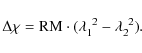
4.2 Distribution of the rotation measure
The polarization angle of the magnetic field vectors is changed by the Faraday
rotation which depends on the square of the wavelength. If the Faraday
depolarization is small, we can calculate the rotation measure (RM) from the
rotation
![]() of the polarization vector between two wavelengths:
of the polarization vector between two wavelengths:
In Fig. 8 we present the RM distribution between
According to the RM distribution the large-scale magnetic field has a
line-of-sight component that is pointing to the observer in the
northeastern half and pointing away from the observer in the
southwestern half. This agrees with a spiral magnetic field in the
disk as expected for a mean-field ![]() -
-![]() dynamo. For an
axisymmetric mode the magnetic field spirals in a uniform direction
(Baryshnikova et al. 1987). Rotation curves show that the northeastern
half is blueshifted whereas the southwestern half is redshifted
(Pence 1981; Puche et al. 1991). Thus, the directions of the velocity and
magnetic field are opposite to each other. Krause & Beck (1998) showed
that for such a case the spiral magnetic field is pointing inwards.
dynamo. For an
axisymmetric mode the magnetic field spirals in a uniform direction
(Baryshnikova et al. 1987). Rotation curves show that the northeastern
half is blueshifted whereas the southwestern half is redshifted
(Pence 1981; Puche et al. 1991). Thus, the directions of the velocity and
magnetic field are opposite to each other. Krause & Beck (1998) showed
that for such a case the spiral magnetic field is pointing inwards.
Using the RM distribution we corrected the magnetic field orientation for the
Faraday rotation. This was also done for the combined VLA + Effelsberg map at
![]() shown in Fig. 5, although
we do not have a RM map with sufficient resolution. We corrected the
polarization angles for angular scales larger than
shown in Fig. 5, although
we do not have a RM map with sufficient resolution. We corrected the
polarization angles for angular scales larger than
![]() using a
combined VLA + Effelsberg RM map (not shown). The Effelsberg polarization maps
at
using a
combined VLA + Effelsberg RM map (not shown). The Effelsberg polarization maps
at
![]()
![]() (Fig. 4) and
(Fig. 4) and
![]() (Fig. 6) could be corrected without loss of resolution.
(Fig. 6) could be corrected without loss of resolution.
The effect of the Faraday correction is especially important at the
the radio spur S1: the magnetic field vectors are almost perpendicular
to the disk after applying the Faraday correction (a RM of
![]() corresponds to a rotation of
corresponds to a rotation of ![]() ). In general the
Faraday correction made the magnetic field orientation more
disk parallel in locations near the disk plane (compare
Figs. 2 and 5).
). In general the
Faraday correction made the magnetic field orientation more
disk parallel in locations near the disk plane (compare
Figs. 2 and 5).
![\begin{figure}
\par\includegraphics[bb=45 160 570 660,width=8.5cm,clip=]{11698fig8_bw}
\end{figure}](/articles/aa/full_html/2009/42/aa11698-09/img90.png)
|
Figure 8:
RM distribution between
|
| Open with DEXTER | |
5 The magnetic field structure
![\begin{figure}
\par\includegraphics[width=18cm,clip=]{11698f9.eps}\par
\end{figure}](/articles/aa/full_html/2009/42/aa11698-09/img91.png)
|
Figure 9:
Profiles of the polarized intensity along the major ( left) and minor axis ( right). The black symbols show the measured
intensities from combined VLA + Effelsberg observations at
|
| Open with DEXTER | |
5.1 Axisymmetric model for the disk magnetic field
In Sect. 3 we suggested that the observed
large-scale magnetic field is the superposition of a disk parallel
and a vertical component. We will refer to the disk-parallel magnetic field with radial and azimuthal ![]() components as the disk magnetic field. The vertical magnetic field with radial and vertical (r,z) components we will refer to as the halo magnetic field.
components as the disk magnetic field. The vertical magnetic field with radial and vertical (r,z) components we will refer to as the halo magnetic field.
As a model for the disk magnetic field we use a spiral magnetic field
corresponding to an axisymmetric spiral (ASS) mode of a galactic dynamo, which
is symmetric with respect to the plane (even parity). The inclination angle of
the disk was prescribed as
![]() ,
which is that of the optical
disk. For a pitch angle of
,
which is that of the optical
disk. For a pitch angle of
![]() the polarized intensity
of our model resembles the observed distribution (the optical pitch angle is
the polarized intensity
of our model resembles the observed distribution (the optical pitch angle is
![]() (Pence 1981)). We fitted the observed polarized intensity
along the major axis with a Gaussian distribution consisting of an inner disk
(
FWHM = 6.5 kpc) and an outer disk (FWHM =13 kpc). For the
vertical polarized emission profile we chose the exponential scaleheight of
the synchrotron emission from the thin disk of
(Pence 1981)). We fitted the observed polarized intensity
along the major axis with a Gaussian distribution consisting of an inner disk
(
FWHM = 6.5 kpc) and an outer disk (FWHM =13 kpc). For the
vertical polarized emission profile we chose the exponential scaleheight of
the synchrotron emission from the thin disk of
![]() at
at ![]()
![]() (Paper I). We assumed energy equipartition between CRs
and the magnetic field (where the CR number density is
(Paper I). We assumed energy equipartition between CRs
and the magnetic field (where the CR number density is
![]() ), so that the Gaussian FWHM and the exponential scaleheight of the magnetic field are two and four times larger, respectively, than that of the
synchrotron emission. The magnetic field has a FWHM of
), so that the Gaussian FWHM and the exponential scaleheight of the magnetic field are two and four times larger, respectively, than that of the
synchrotron emission. The magnetic field has a FWHM of
![]() and
and
![]() in the inner and outer disk, respectively, and a vertical
scaleheight of
in the inner and outer disk, respectively, and a vertical
scaleheight of
![]() .
The profiles of the polarized flux density of
the model and the observations are presented in Fig. 9. A
summary of the model parameters can be found in
Table 3.
.
The profiles of the polarized flux density of
the model and the observations are presented in Fig. 9. A
summary of the model parameters can be found in
Table 3.
We produced maps of Stokes Q and U by integrating along the line-of-sight
where
The model of the disk magnetic field clearly shows why the polarized emission is not symmetric with respect to the major and minor axis: the locations of the maxima of the polarized intensity are shifted due to the pitch angle in counterclockwise direction from the minor axis. Hence, the polarized intensity distribution resembles an S-shape, as observed. The depolarized regions D1 and D2 in the observed map of the polarized intensity (Fig. 5) can be explained by the model, too. They are located where different components of the magnetic field occur in one beam and thus cancel each other. We note that the magnetic field orientation is mainly disk parallel as expected for a spiral magnetic field. The good agreement between the model and the observed distribution in the disk justifies the choice of the model.
The comparison of the profiles of the polarized emission between the observations and the model in Fig. 9 shows that along the minor axis the halo shows up as additional emission. The halo magnetic field is investigated in the next section.
5.2 The halo magnetic field
The good agreement in the disk region of the simple model shown in Fig. 10 with the observations shows that the disk field dominates in the disk. We note that the two radio spurs are located near the two depolarized regions (D1 and D2 in Fig. 5), where the projected disk field has a minimum. Elsewhere the visibility of the halo field is reduced by the dominating disk field.
The observed polarized emission is the superposition of the disk
and halo component with
![]() and
and
![]() .
We subtracted the disk magnetic field model
from the maps of Stokes Q and U of the combined VLA +
Effelsberg observations at
.
We subtracted the disk magnetic field model
from the maps of Stokes Q and U of the combined VLA +
Effelsberg observations at
![]() .
The polarized
intensity and the orientation of the halo magnetic field was
calculated from the maps of
.
The polarized
intensity and the orientation of the halo magnetic field was
calculated from the maps of ![]() and
and ![]() and is
presented in Fig. 11.
and is
presented in Fig. 11.
The halo magnetic field clearly resembles an X-shape centered on
the nucleus. Its orientation is mirror symmetric both to the major and
minor axis. X-shaped halo fields have been observed in several edge-on
galaxies with inclination angles
![]() ,
almost edge-on
(Krause et al. 2006; Krause 2007). This is the first galaxy with an X-shaped field which is only mildly edge-on (
,
almost edge-on
(Krause et al. 2006; Krause 2007). This is the first galaxy with an X-shaped field which is only mildly edge-on (
![]() ),
so that the emission from the disk and halo are superimposed.
),
so that the emission from the disk and halo are superimposed.
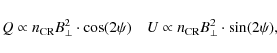
In order to quantify the halo magnetic field we determined the
mean orientation angle
![]() in the four boxes shown in
Fig. 11. We integrated Stokes Q and
U and calculated the orientation angle of the magnetic field by
in the four boxes shown in
Fig. 11. We integrated Stokes Q and
U and calculated the orientation angle of the magnetic field by
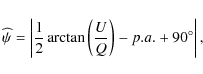
where
5.3 Modeling the rotation measure distribution
An analysis of the RMs, averaged in sectors, as a function of the azimuthal
angle ![]() gives further information about the structure of the
large-scale magnetic field. The sector integration was applied between a
galactocentric radius of
gives further information about the structure of the
large-scale magnetic field. The sector integration was applied between a
galactocentric radius of
![]() and
and
![]() with a spacing
of
with a spacing
of ![]() in the azimuthal angle (see Fig. 8). An
effective inclination of
in the azimuthal angle (see Fig. 8). An
effective inclination of
![]() describes the observed distribution of the
polarized emission in the disk and halo at
describes the observed distribution of the
polarized emission in the disk and halo at ![]()
![]() with
with
![]() resolution (Fig. 4). We
chose the RM distribution at
resolution (Fig. 4). We
chose the RM distribution at
![]() resolution, because the low
resolution favors the study of the large-scale RM structure.
resolution, because the low
resolution favors the study of the large-scale RM structure.
The crosses in Fig. 12 give the azimuthal RM variation
together with their errors. There is a broad maximum between
![]() and
and
![]() and the minimum is near
and the minimum is near
![]() .
This confirms the result
previously obtained from the morphology of the RM distribution: the
northeastern half of the galaxy contains positive RMs
(
.
This confirms the result
previously obtained from the morphology of the RM distribution: the
northeastern half of the galaxy contains positive RMs
(
![]() )
whereas the southwestern half of
the galaxy contains negative RMs (
)
whereas the southwestern half of
the galaxy contains negative RMs (
![]() ).
).
The disk magnetic field is dominating the polarized emission. Therefore we
will use the ASS model of the disk magnetic field in order to make a model for
the RM distribution. We integrated the polarization vector along the
line-of-sight, so that we take Faraday depth effects into account
(Sokoloff et al. 1998). From the Emission Measure
![]() (Hoopes et al. 1996) we derived an electron density of
(Hoopes et al. 1996) we derived an electron density of
![]() ,
where we assumed a pathlength of
,
where we assumed a pathlength of
![]() .
From the H
.
From the H![]() distribution we derived a Gaussian distribution of the electron density along
the major axis with a FWHM of 13 kpc and a vertical scaleheight of 1.4 kpc.
The RM distribution of the ASS model is presented in
Fig. 13. It is notably asymmetric where the minimum
has a larger amplitude than the maximum.
distribution we derived a Gaussian distribution of the electron density along
the major axis with a FWHM of 13 kpc and a vertical scaleheight of 1.4 kpc.
The RM distribution of the ASS model is presented in
Fig. 13. It is notably asymmetric where the minimum
has a larger amplitude than the maximum.
Averaging Stokes Q and U of our ASS magnetic field model in sectors
provides the azimuthal RM variation shown as solid line in
Fig. 12. We found reasonable agreement with the observed
variation for an ordered magnetic field strength of
![]() .
From pulsar RMs we obtain a foreground of
.
From pulsar RMs we obtain a foreground of
![]() at the position of NGC 253, which is near to the Galactic south
pole (Noutsos et al. 2008). Compared with the amplitude of the RM variation the
foreground RM is
at the position of NGC 253, which is near to the Galactic south
pole (Noutsos et al. 2008). Compared with the amplitude of the RM variation the
foreground RM is ![]() 10%, which we further neglect in our analysis.
10%, which we further neglect in our analysis.
The azimuthal RM variation of a spiral ASS field in an RM screen or a
homogeneous, mildly inclined emitting layer can be described by a simple
cosine, with a phase shift
![]() equal to the pitch angle of the
magnetic field spiral (Krause et al. 1989). However, the strongly inclined disk
of NGC 253 requires to take into account the distribution of Faraday depths
along the line-of-sight.
equal to the pitch angle of the
magnetic field spiral (Krause et al. 1989). However, the strongly inclined disk
of NGC 253 requires to take into account the distribution of Faraday depths
along the line-of-sight.
Table 3: Parameters used for the ASS model of the disk magnetic field.
![\begin{figure}
\par\includegraphics[bb=35 175 570 640,width=8.5cm,clip]{11698fig10}
\end{figure}](/articles/aa/full_html/2009/42/aa11698-09/img129.png)
|
Figure 10:
Modeled polarized intensity at
|
| Open with DEXTER | |
![\begin{figure}
\par\includegraphics[bb=35 175 570 640,width=8.5cm,clip]{11698fig11}
\end{figure}](/articles/aa/full_html/2009/42/aa11698-09/img130.png)
|
Figure 11:
Polarized intensity at |
| Open with DEXTER | |
![\begin{figure}
\includegraphics[width=9cm,clip]{11698f12.eps}
\end{figure}](/articles/aa/full_html/2009/42/aa11698-09/img131.png)
|
Figure 12:
RM variation as a function of the azimuthal angle |
| Open with DEXTER | |
![\begin{figure}
\par\resizebox{\hsize}{!}{
\includegraphics[bb=30 160 570 660,width=8.5cm,clip]{11698fig13_bw}}\vfill\end{figure}](/articles/aa/full_html/2009/42/aa11698-09/img134.png)
|
Figure 13:
RM distribution of the axisymmetric spiral (ASS) of the disk magnetic field at
|
| Open with DEXTER | |
Our model can explain the observations much better than the cosine variation
of an RM screen. For the screen the amplitudes of the maximum and the minimum
are equal, whereas our model can reproduce both the maximum with
![]() and the minimum
and the minimum
![]() .
Furthermore, the RM screen predicts the maximum at
.
Furthermore, the RM screen predicts the maximum at
![]() but our model shows that the maximum is very broad, in
agreement with the observations. This can be explained by the thickness of the
disk (not a thin emitting layer) and the inclination of the disk together with
the smearing by the observation beam. The difference in amplitude between the
maximum and minimum is a strong function of inclination.
but our model shows that the maximum is very broad, in
agreement with the observations. This can be explained by the thickness of the
disk (not a thin emitting layer) and the inclination of the disk together with
the smearing by the observation beam. The difference in amplitude between the
maximum and minimum is a strong function of inclination.
The model of the disk magnetic field alone fits already to the observed RM
variation (reduced
![]() ). But so far we took not into account the halo
magnetic field that we also observe and which contributes significantly to the
polarized emission. With observations at only two wavelengths there is no
direct way to decompose the observed RM of the disk and halo magnetic field,
because they are overlapping along the line-of-sight. Still, we can produce a
model including the halo and disk magnetic fields.
). But so far we took not into account the halo
magnetic field that we also observe and which contributes significantly to the
polarized emission. With observations at only two wavelengths there is no
direct way to decompose the observed RM of the disk and halo magnetic field,
because they are overlapping along the line-of-sight. Still, we can produce a
model including the halo and disk magnetic fields.
For the halo magnetic field we propose a model where the field lines are along
a cone above and below the galactic plane, so that in projection to the plane
of the sky the field forms an X-shape. From the orientation angle of the halo
magnetic field as derived in Sect. 5.2 we deduce an opening
angle of the cone of
![]() .
Note that the contributions to the RM do not cancel if the
line-of-sight components of the field change sign along the
line-of-sight, as is the case in our cone model, because of different
pathlengths towards the cone's far and near sides. Hence, we see the RM
mainly from the front half of the cone.
.
Note that the contributions to the RM do not cancel if the
line-of-sight components of the field change sign along the
line-of-sight, as is the case in our cone model, because of different
pathlengths towards the cone's far and near sides. Hence, we see the RM
mainly from the front half of the cone.
![\begin{figure}
\par\includegraphics[width=8.5cm,clip]{11698fig14}
\end{figure}](/articles/aa/full_html/2009/42/aa11698-09/img139.png)
|
Figure 14:
Modeled polarized intensity at |
| Open with DEXTER | |
![\begin{figure}
\par\includegraphics[width=8cm,clip]{11698fig15_bw}
\end{figure}](/articles/aa/full_html/2009/42/aa11698-09/img141.png)
|
Figure 15:
Model RM distribution for the combined even disk and even halo magnetic field at
|
| Open with DEXTER | |
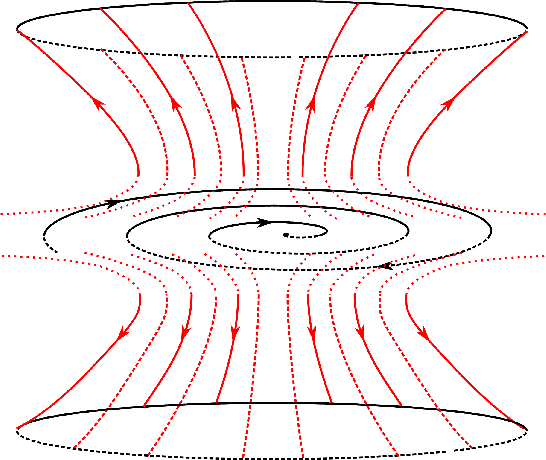
|
Figure 16: Sketch of the observable components of the large-scale magnetic field structure. In the disk, the ASS spiral magnetic field is even and pointing inwards. In the halo, the magnetic field is also even and pointing outwards. Dashed lines indicate components on the rear side. The dotted part of the halo magnetic field is not observed. |
| Open with DEXTER | |
For the same reason we can only see the field direction in the southern halo,
because it lies in front of the bright disk and acts therefore as a Faraday
screen. Our models show that the magnetic field points away from the disk in
the southern halo. In case that the field points also away from the disk in
the northern halo, the halo field has even parity. Otherwise, if the
field points towards the disk in the northern halo, the halo field has
odd parity. Because the field direction in the northern halo has only a
small influence on the RM distribution the difference of the azimuthal RM
variation is also small. We tested all possible combinations of disk and halo
magnetic field configurations. The result is summarized in a catalog in
Appendix A. The disk magnetic field is of even parity, where
the field is pointing in the same direction above and below the galactic
midplane. An odd disk magnetic field in combination with any halo magnetic
field leads to strong local gradients in the RM distribution which are not
observed. The even disk field together with an even halo field fits slightly
better to the observations with a reduced
![]() (see
Fig. 12) than with an odd halo field with
(see
Fig. 12) than with an odd halo field with ![]() (see
Fig. A.7). The polarized intensity and the RM distribution of
our favored model for the combined even disk and even halo magnetic field is
shown in Figs. 14 and 15. A
sketch of the magnetic field lines is presented in
Fig. 16
(see
Fig. A.7). The polarized intensity and the RM distribution of
our favored model for the combined even disk and even halo magnetic field is
shown in Figs. 14 and 15. A
sketch of the magnetic field lines is presented in
Fig. 16![]() .
.
We investigated also the possibility of an azimuthal halo magnetic field
component which is predicted by some halo models
(Wang & Abel 2009; Dalla Vecchia & Schaye 2008). It was included into the conical magnetic
field model and the RM variation of the combined disk and halo model was
studied. It turned out that the azimuthal component - if there is any - must
point in the opposite direction to that of the disk magnetic field. As an
upper limit of the azimuthal component we estimate 60% of the field
strength (
![]() ). We note that the shape and direction of the model
halo magnetic field is still consistent with the observations, i.e. is not
very sensitive to the relative strength of the azimuthal component.
). We note that the shape and direction of the model
halo magnetic field is still consistent with the observations, i.e. is not
very sensitive to the relative strength of the azimuthal component.
5.4 Magnetic field strengths
The magnetic field strength can be calculated using the energy equipartition
assumption as described in Beck & Krause (2005). As in Paper I we use a pathlength
through the total power emission of 6.5 kpc and a CR proton to electron ratio
of K=100, and a nonthermal radio spectral index of 1.0. With a typical
nonthermal total power flux density of 8 mJy/beam at ![]() 6.2 cm with
30
6.2 cm with
30
![]() resolution we find a total magnetic field strength of
resolution we find a total magnetic field strength of
![]() in the disk. At a polarization degree of
in the disk. At a polarization degree of ![]() this
corresponds to
this
corresponds to
![]() for the ordered magnetic field in the
disk. The strength of the halo magnetic field was estimated by fitting
profiles of the polarized emission to the observations (see
Fig. 9). We found
for the ordered magnetic field in the
disk. The strength of the halo magnetic field was estimated by fitting
profiles of the polarized emission to the observations (see
Fig. 9). We found
![]() for the halo magnetic
field.
for the halo magnetic
field.
We now compare the magnetic field strengths of the ordered field calculated
from the equipartition and from the RM analysis. The equipartition value can
be larger than that of the RM analysis, because the anisotropic turbulent
magnetic field emits polarized emission but does not or only weakly contribute
to the observed RM (Beck et al. 2005). From the azimuthal RM variation of our
modeled ASS disk field we found an ordered magnetic field component of
![]() for the disk. In the halo, the magnetic field strength
is similar with
for the disk. In the halo, the magnetic field strength
is similar with
![]() .
There may be some anisotropic field
component both in the disk and halo because the equipartition strength of the
ordered magnetic field is about 50% larger than that of the RM
analysis. The anisotropic field component can contribute significantly to the
polarized emission in galaxies as shown for NGC 1097 (Beck et al. 2005) and M 51 (Fletcher et al. 2010).
.
There may be some anisotropic field
component both in the disk and halo because the equipartition strength of the
ordered magnetic field is about 50% larger than that of the RM
analysis. The anisotropic field component can contribute significantly to the
polarized emission in galaxies as shown for NGC 1097 (Beck et al. 2005) and M 51 (Fletcher et al. 2010).
6 Discussion
6.1 The superwind model
NGC 253 is a prototypical nuclear starburst galaxy, which
is the source of an outflow of hot X-ray emitting gas
(Bauer et al. 2007; Strickland et al. 2000). Spectroscopic measurements of
H![]() -emitting gas in the southern nuclear outflow cone by
Schulz & Wegner (1992) give an outflow velocity of
-emitting gas in the southern nuclear outflow cone by
Schulz & Wegner (1992) give an outflow velocity of
![]() .
Apart from the nuclear outflow, huge lobes of
diffuse X-ray emission in the halo are extending up to
.
Apart from the nuclear outflow, huge lobes of
diffuse X-ray emission in the halo are extending up to ![]() away from
the disk. These lobes are thought to be the walls of two huge
bubbles containing a hot gas with a low density (Strickland et al. 2002; Pietsch et al. 2000). Sensitive XMM-Newton observations revealed that
indeed the entire bubbles are filled with X-ray emitting gas
(Bauer et al. 2008). Similar structures are found in other galaxies with
intense star formation, with M 82 as the most prominent example,
and are now known as superwinds (Heckman et al. 2000).
away from
the disk. These lobes are thought to be the walls of two huge
bubbles containing a hot gas with a low density (Strickland et al. 2002; Pietsch et al. 2000). Sensitive XMM-Newton observations revealed that
indeed the entire bubbles are filled with X-ray emitting gas
(Bauer et al. 2008). Similar structures are found in other galaxies with
intense star formation, with M 82 as the most prominent example,
and are now known as superwinds (Heckman et al. 2000).
Figure 17 shows the diffuse H![]() emission in
greyscale. There are several H
emission in
greyscale. There are several H![]() plumes extending from the disk into the
halo. We note that the large plume east of the nucleus corresponds to the
radio spur S1 (see Fig. 5). The diffuse X-ray emission in Fig. 18 shows a similar structure with the
lobe at the extension E1 extending furthest into the halo. The abundance of
heated gas has an asymmetry with respect to the minor axis: the northeastern
half contains significantly more diffuse H
plumes extending from the disk into the
halo. We note that the large plume east of the nucleus corresponds to the
radio spur S1 (see Fig. 5). The diffuse X-ray emission in Fig. 18 shows a similar structure with the
lobe at the extension E1 extending furthest into the halo. The abundance of
heated gas has an asymmetry with respect to the minor axis: the northeastern
half contains significantly more diffuse H![]() and soft X-ray emission than the southwestern half which cannot be explained by a symmetric
superwind. This asymmetry is also observed in H I emission
(Boomsma et al. 2005) which surrounds the superbubbles. An explanation is
attempted in Sect. 6.4.
and soft X-ray emission than the southwestern half which cannot be explained by a symmetric
superwind. This asymmetry is also observed in H I emission
(Boomsma et al. 2005) which surrounds the superbubbles. An explanation is
attempted in Sect. 6.4.
6.2 The disk wind model
The halo magnetic field allows CRs to stream along the field lines from the
disk into the halo. In Paper I we determined the vertical CR bulk speed as
![]() which is remarkably constant over
the entire extent of the disk. This shows the existence of a disk wind in
NGC 253. CRs cannot stream faster than with Alfvén speed with respect to
the magnetic field, because they are scattered at self-excited Alfvén
waves via the so-called streaming instability (Kulsrud & Pearce 1969). A typical
magnetic field strength of
which is remarkably constant over
the entire extent of the disk. This shows the existence of a disk wind in
NGC 253. CRs cannot stream faster than with Alfvén speed with respect to
the magnetic field, because they are scattered at self-excited Alfvén
waves via the so-called streaming instability (Kulsrud & Pearce 1969). A typical
magnetic field strength of
![]() and a density of the warm
gas of
and a density of the warm
gas of
![]() (Sect. 3.5) leads to an Alfvén speed of
(Sect. 3.5) leads to an Alfvén speed of
![]() .
The super-Alfvénic CR bulk speed requires that the CRs and the magnetic
field are advectively transported together in the disk wind. CRs stream
with Alfvén speed with
respect to the magnetic field that is frozen into the thermal gas of
the
wind. The measured CR bulk speed is the superposition
.
The super-Alfvénic CR bulk speed requires that the CRs and the magnetic
field are advectively transported together in the disk wind. CRs stream
with Alfvén speed with
respect to the magnetic field that is frozen into the thermal gas of
the
wind. The measured CR bulk speed is the superposition
![]() of the outflow speed of the thermal
gas
of the outflow speed of the thermal
gas
![]() in the wind and the Alfvén speed
in the wind and the Alfvén speed
![]() (Breitschwerdt et al. 2002). Adopting this picture the wind speed at the
galactic midplane in NGC 253 is
(Breitschwerdt et al. 2002). Adopting this picture the wind speed at the
galactic midplane in NGC 253 is
![]() .
.
![\begin{figure}
\par\includegraphics[width=8.5cm,clip]{11698fig17.eps}
\end{figure}](/articles/aa/full_html/2009/42/aa11698-09/img161.png)
|
Figure 17:
Halo magnetic field overlaid onto diffuse H |
| Open with DEXTER | |
![\begin{figure}
\par\includegraphics[width=8.5cm,clip]{11698fig18}
\end{figure}](/articles/aa/full_html/2009/42/aa11698-09/img164.png)
|
Figure 18:
Halo magnetic field overlaid onto diffuse X-ray emission. The contour is at
|
| Open with DEXTER | |
If the large-scale magnetic field is frozen into the thermal gas in the wind the halo magnetic field has an azimuthal component and winds up in a spiral. The field configuration is similar to that of the sun with the Parker spiral magnetic field (Weber & Davis 1967; Parker 1958). The azimuthal component increases with height, so that above a certain height the magnetic field is almost purely azimuthal. Up to the Alfvénic point the stiff magnetic field lines corotate with the underlying disk. If the azimuthal component of the halo magnetic field is small, the observable radio halo is within the corotating regime and the Alfvén radius is larger than the vertical extent of the halo. As an azimuthal halo component cannot be excluded (Sect. 5.3), the Alfvénic radius may be smaller than 2 kpc, which is the scaleheight of the polarized emission in the halo.
The existence of a disk wind has important consequences for the transport of
angular momentum. As we have shown in Paper I the CR bulk speed is fairly
constant over the extent of the disk, i.e. it does not depend on the
galactocentric radius. If this is also true for the speed of the disk wind,
angular momentum is effectively transported to large galactocentric radii
(Zirakashvili et al. 1996). Moreover, the angular momentum of the wind per unit
wind mass is proportional to the Alfvén radius as shown by
Zirakashvili et al. (1996). An Alfvén radius of ![]()
![]() agrees
with their models for which they found a significant loss of angular momentum
over the lifetime of a galaxy. We note that the disk wind can account for
larger angular momentum losses than the superwind in the center (at small
galactocentric radii).
agrees
with their models for which they found a significant loss of angular momentum
over the lifetime of a galaxy. We note that the disk wind can account for
larger angular momentum losses than the superwind in the center (at small
galactocentric radii).
6.3 The origin of X-shaped halo magnetic fields
The distribution of the halo magnetic field is X-shaped in both orientation and intensity. As the intensity of the polarized emission depends on the perpendicular component of the ordered field, a possible explanation of the intensity distribution is limb brightening in the conical halo magnetic field. We modeled this effect using a halo magnetic field lying on a cone with an opening angle ofThe halo magnetic field follows the lobes of the heated gas that are
regarded as walls of huge bubbles expanding into the surrounding
medium. The large-scale magnetic field may be compressed and aligned
by shock waves in the walls. These shock waves are also able to heat a
pre-existing cold halo gas, so that the gas becomes visible as
H![]() and soft X-ray emission. The cold halo gas seen in
H I emission surrounds the superbubbles and shows the same
asymmetric distribution as expected if this gas is the source for the
heated gas in the halo. A cartoon of the halo structure including the
large-scale magnetic field is shown in
Fig. 19.
and soft X-ray emission. The cold halo gas seen in
H I emission surrounds the superbubbles and shows the same
asymmetric distribution as expected if this gas is the source for the
heated gas in the halo. A cartoon of the halo structure including the
large-scale magnetic field is shown in
Fig. 19.
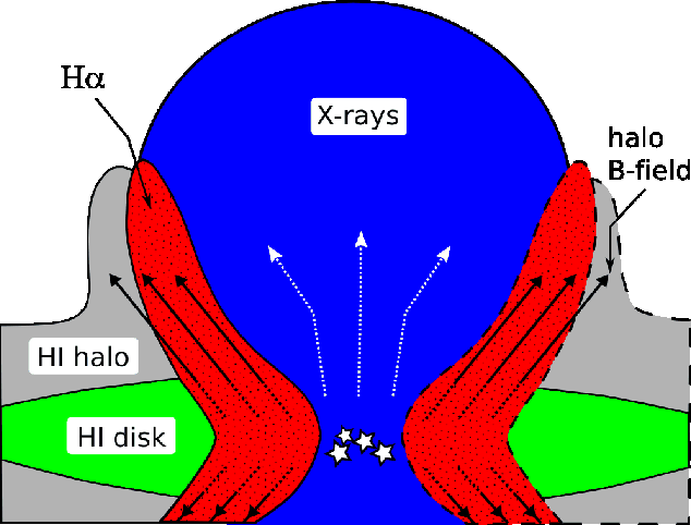
|
Figure 19: Halo structure of NGC 253. Reproduced from Boomsma et al. (2005) and extended. The superbubble, filled with soft X-rays emitting gas, expands into the surrounding medium (indicated by dotted lines with arrows). The halo magnetic field is aligned with the walls of the superbubble. Dashed lines denote components that are not (or only weakly) detected in the southwestern half of NGC 253. |
| Open with DEXTER | |
Both the disk wind model and the superwind model, in conjunction with
a large-scale dynamo action, can explain the X-shaped halo magnetic
field. We should note, however, that such magnetic field structures
are observed in several edge-on galaxies. These galaxies show a very
different level of star formation (Krause 2009). Most of them do
not possess a starburst in the center and hence they have no
superwind. While the classical ![]() -
-![]() dynamo can not
explain such an X-shaped halo field, model calculations of a galactic
disk within a spherical halo including a galactic wind showed a
similar magnetic field configuration
(Brandenburg et al. 1993). Hydrodynamical simulations show that the wind
in spiral galaxies has a significant radial component due to the
radial gradient of the gravitational potential. The wind flow reveals
an X-shape when the galaxy is seen edge-on
(Dalla Vecchia & Schaye 2008). New MHD simulations of disk galaxies
including a galactic wind are in progress and may explain the halo
X-shaped field (Gressel et al. 2008; Hanasz et al. 2009b,a). The first
global galactic-scale MHD simulations of a CR-driven dynamo
give very promising results showing directly that magnetic flux is
transported from the disk into the halo (Hanasz et al. 2009c). Therefore
we suggest that in NGC 253 the X-shaped halo field is connected
rather to the disk wind than to the superwind. The superwind gas flow
may be collimated by the halo magnetic field.
dynamo can not
explain such an X-shaped halo field, model calculations of a galactic
disk within a spherical halo including a galactic wind showed a
similar magnetic field configuration
(Brandenburg et al. 1993). Hydrodynamical simulations show that the wind
in spiral galaxies has a significant radial component due to the
radial gradient of the gravitational potential. The wind flow reveals
an X-shape when the galaxy is seen edge-on
(Dalla Vecchia & Schaye 2008). New MHD simulations of disk galaxies
including a galactic wind are in progress and may explain the halo
X-shaped field (Gressel et al. 2008; Hanasz et al. 2009b,a). The first
global galactic-scale MHD simulations of a CR-driven dynamo
give very promising results showing directly that magnetic flux is
transported from the disk into the halo (Hanasz et al. 2009c). Therefore
we suggest that in NGC 253 the X-shaped halo field is connected
rather to the disk wind than to the superwind. The superwind gas flow
may be collimated by the halo magnetic field.
The transport of CRs and magnetic fields has important
consequences for the possibility of a working dynamo in NGC 253.
The ![]() -
-![]() dynamo relies on the differential rotation of
the galactic disk (
dynamo relies on the differential rotation of
the galactic disk (![]() -effect) and the cyclonic motions of the
ionized gas (
-effect) and the cyclonic motions of the
ionized gas (![]() -effect). The latter one can be generated by
subsequent supernova explosions (Ferrière 1992). The
amplification of magnetic fields by an
-effect). The latter one can be generated by
subsequent supernova explosions (Ferrière 1992). The
amplification of magnetic fields by an ![]() -
-![]() dynamo
requires expulsion of small-scale helical fields (see
e.g. Brandenburg & Subramanian 2005). Sur et al. (2007) showed that galactic
winds can transport the helicity flux by advection. A galactic wind
may be thus vital for a working dynamo.
dynamo
requires expulsion of small-scale helical fields (see
e.g. Brandenburg & Subramanian 2005). Sur et al. (2007) showed that galactic
winds can transport the helicity flux by advection. A galactic wind
may be thus vital for a working dynamo.
6.4 The origin of the gas in the halo
The cold gas in the halo of NGC 253 is necessary to explain the halo structure with the superwind model. Its origin, however, is yet unknown. Boomsma et al. (2005) discussed a gas infall in NGC 253 by a minor merger to explain the asymmetric H I halo distribution with respect to the minor axis. But they noted that a minor merger event is unlikely because the distribution of H I is very symmetric with respect to the major axis. Could the disk wind be the origin of the cold gas in the halo? The disk wind is asymmetric with respect to the minor axis. The convective northeastern half indicates a strong disk wind which transports gas from the disk into the halo while in the diffusive southwestern half the wind is weaker (Paper I).
We can only speculate about the reason why the two halo parts are so different. Star formation in the disk most likely plays an important role. The northeastern spiral arm contains significantly more H II regions than the southwestern one as is visible from Fig. 4b in Hoopes et al. (1996). Moreover, the amount of total radio continuum emission indicates a higher star-formation rate in this part of the disk. Since the energy input of star formation is essential for the injection of thermal and CR gas, the disk wind can be more easily driven in the northeastern half. Thus, the disk wind is a good candidate for the origin of the cold gas in the halo.
7 Summary and conclusions
The three-dimensional magnetic field structure can be investigated using sensitive radio continuum polarimetry. Our main results are:
- 1.
- A disk parallel magnetic field exists along the midplane of the disk. The magnetic field lines are slowly opening further away from the midplane. The vertical magnetic field component is most prominent at the edge of the inner disk where we find two ``radio spurs'', one previously known east of the nucleus and one newly discovered west of the nucleus. The magnetic field configuration can be described as an X-shaped pattern, as in other edge-on galaxies.
- 2.
- The large-scale magnetic field can be decomposed into a disk
 and a halo (r,z) component.
- 3.
- The disk magnetic field of NGC 253 can be described by an axisymmetric
spiral (ASS) magnetic field with a constant pitch angle of
 which is symmetric with respect to the plane. This
model shows a high resemblance to the observed magnetic field in the disk.
which is symmetric with respect to the plane. This
model shows a high resemblance to the observed magnetic field in the disk.
- 4.
- The distribution of the polarized intensity and the
orientation of the halo magnetic field shows a distinct X-shaped
pattern centered on the nucleus. Our model of the disk magnetic
field was subtracted to construct a map of the halo magnetic field.
We propose a model where the halo field lines are along a cone with
an opening angle of
 and are pointing away from
the disk (even parity). An odd halo magnetic field is also possible,
because we can not reliably determine the magnetic field direction in
the northern halo.
and are pointing away from
the disk (even parity). An odd halo magnetic field is also possible,
because we can not reliably determine the magnetic field direction in
the northern halo.
- 5.
- The distribution of the halo magnetic field coincides in shape
with the extra-planar heated gas traced by H
 and soft X-ray
emission. Possible explanations are limb brightening and compression
of the halo magnetic field in the walls of the expanding
superbubbles.
and soft X-ray
emission. Possible explanations are limb brightening and compression
of the halo magnetic field in the walls of the expanding
superbubbles.
- 6.
- A disk wind plus dynamo action is a promising scenario for the origin of the gas in the halo and for the expulsion of small-scale helical fields as requested for efficient dynamo action. The disk wind can also account for large angular momentum and magnetic flux losses over galactic time scales.
VH acknowledges the funding by the Graduiertenkolleg GRK 787 and the Sonderforschungsbereich SFB 591 during the course of his PhD. The GRK 787 ``Galaxy groups as laboratories for baryonic and dark matter'' and the SFB 591 ``Universal properties of non-equilibrium plasmas'' are funded by the Deutsche Forschungsgemeinschaft (DFG). RJD is supported by DFG in the framework of the research unit FOR 1048.
We thank Dieter Breitschwerdt and Andrew Fletcher for many fruitful discussions. Moreover, we would like to thank Charles Hoopes for kindly providing us his H
References
- Baryshnikova, I., Shukurov, A., Ruzmaikin, A., et al. 1987, A&A, 177, 27 [NASA ADS]
- Bauer, M., Pietsch, W., Trinchieri, G., et al. 2007, A&A, 467, 979 [NASA ADS] [CrossRef] [EDP Sciences]
- Bauer, M., Pietsch, W., Trinchieri, G., et al. 2008, A&A, 489, 1029 [NASA ADS] [CrossRef] [EDP Sciences]
- Beck, R. 2007, A&A, 470, 539 [NASA ADS] [CrossRef] [EDP Sciences]
- Beck, R., & Krause, M. 2005, AN, 326, 414 [NASA ADS]
- Beck, R., Carilli, C. L., Holdaway, M. A., et al. 1994, A&A, 292, 409 [NASA ADS]
- Beck, R., Brandenburg, A., Moss, D., Shukurov, A., & Sokoloff, D. 1996, ARA&A, 34, 155 [NASA ADS] [CrossRef]
- Beck, R., Fletcher, A., Shukurov, A., et al. 2005, A&A, 444, 739 [NASA ADS] [CrossRef] [EDP Sciences]
- Boomsma, R., Oosterloo, T., Fraternali, F., van der Hulst, J. M., & Sancisi, R. 2005, A&A, 431, 65 [NASA ADS] [CrossRef] [EDP Sciences]
- Brandenburg, A., & Subramanian, K. 2005, Phys. Rep., 417, 1 [NASA ADS] [CrossRef]
- Brandenburg, A., Donner, K. J., Moss, D., et al. 1993, A&A, 271, 36 [NASA ADS]
- Braun, R. 1988, Millimeter Array Memo, 46
- Breitschwerdt, D. 2003, in Rev. Mex. Astron. Astrofis. Conf. Ser. 15, ed. J. Arthur, & W. J. Henney, 311
- Breitschwerdt, D., McKenzie, J. F., & Völk, H. J. 1991, A&A, 245, 79 [NASA ADS]
- Breitschwerdt, D., McKenzie, J. F., & Völk, H. J. 1993, A&A, 269, 54 [NASA ADS]
- Breitschwerdt, D., Dogiel, V. A., & Völk, H. J. 2002, A&A, 385, 216 [NASA ADS] [CrossRef] [EDP Sciences]
- Brentjens, M. A., & de Bruyn, A. G. 2005, A&A, 441, 1217 [NASA ADS] [CrossRef] [EDP Sciences]
- Carilli, C. L., Holdaway, M. A., Ho, P. T. P., et al. 1992, ApJ, 399, L59 [NASA ADS] [CrossRef]
- Chyzy, K. T. 2008, A&A, 482, 755 [NASA ADS] [CrossRef] [EDP Sciences]
- Chyzy, K. T., & Beck, R. 2004, A&A, 417, 541 [NASA ADS] [CrossRef] [EDP Sciences]
- Chyzy, K. T., Ehle, M., & Beck, R. 2007, A&A, 474, 415 [NASA ADS] [CrossRef] [EDP Sciences]
- Dahlem, M., Lisenfeld, U., & Golla, G. 1995, ApJ, 444, 119 [NASA ADS] [CrossRef]
- Dahlem, M., Lisenfeld, U., & Rossa, J. 2006, A&A, 457, 121 [NASA ADS] [CrossRef] [EDP Sciences]
- Dalla Vecchia, C., & Schaye, J. 2008, MNRAS, 387, 1431 [NASA ADS] [CrossRef]
- Dettmar, R.-J. 1992, Fundamentals of Cosmic Physics, 15, 143 [NASA ADS]
- Dettmar, R.-J., & Soida, M. 2006, AN, 327, 495 [NASA ADS]
- Dumke, M., & Krause, M. 1998, in The Local Bubble and Beyond, ed. D. Breitschwerdt, M. J. Freyberg, & J. Trümper, Lect. Notes Phys. 506 (Berlin: Springer Verlag), IAU Colloq., 166, 555
- Everett, J. E., Zweibel, E. G., Benjamin, R. A., et al. 2008, ApJ, 674, 258 [NASA ADS] [CrossRef]
- Ferrière, K. 1992, ApJ, 391, 188 [NASA ADS] [CrossRef]
- Fletcher, A., Beck, R., Shukurov, A., Berkhuijsen, E. M. & Horellou, C. 2010, in prep.
- Golla, G., & Hummel, E. 1994, A&A, 284, 777 [NASA ADS]
- Gressel, O., Elstner, D., Ziegler, U., et al. 2008, A&A, 486, L35 [NASA ADS] [CrossRef] [EDP Sciences]
- Hanasz, M., Otmianowska-Mazur, K., Kowal, G., et al. 2009a, A&A, 498, 335 [NASA ADS] [CrossRef] [EDP Sciences]
- Hanasz, M., Otmianowska-Mazur, K., Lesch, H., et al. 2009b, in IAU Symp., 259, 479
- Hanasz, M., Wóltanski, D., Kowalik, K., et al. 2009c, in IAU Symp., 259, 549
- Heald, G., Braun, R., & Edmonds, R. 2009, A&A, 503, 409 [NASA ADS] [CrossRef] [EDP Sciences]
- Heckman, T. M., Lehnert, M. D., Strickland, D. K., et al. 2000, ApJS, 129, 493 [NASA ADS] [CrossRef]
- Heesen, V. 2008, Ph.D. Thesis, Ruhr-Universität Bochum, Germany
- Heesen, V., Beck, R., Krause, M., et al. 2009, A&A, 494, 563 [NASA ADS] [CrossRef] [EDP Sciences]
- Hoopes, C. G., Walterbos, R. A. M., & Greenwalt, B. E. 1996, AJ, 112, 1429 [NASA ADS] [CrossRef]
- Ipavich, F. M. 1975, ApJ, 196, 107 [NASA ADS] [CrossRef]
- Karachentsev, I. D., Grebel, E. K., Sharina, M. E., et al. 2003, A&A, 404, 93 [NASA ADS] [CrossRef] [EDP Sciences]
- Krause, F., & Beck, R. 1998, A&A, 335, 789 [NASA ADS]
- Krause, M. 2004, in The Magnetized Interstellar Medium, ed. B. Uyaniker, W. Reich, & R. Wielebinski, 173
- Krause, M. 2007, in Mem. della Soc. Astron. Ital., 78, 314
- Krause, M. 2009, in , Magnetic Fields in the Universe II, ed. A. Esquivel, RevMexAA, 36, 25
- Krause, M., Hummel, E., & Beck, R. 1989, A&A, 217, 4 [NASA ADS]
- Krause, M., Wielebinski, R., & Dumke, M. 2006, A&A, 448, 133 [NASA ADS] [CrossRef] [EDP Sciences]
- Kulsrud, R., & Pearce, W. P. 1969, ApJ, 156, 445 [NASA ADS] [CrossRef]
- Mac Low, M.-M., & Ferrara, A. 1999, ApJ, 513, 142 [NASA ADS] [CrossRef]
- Norman, C. A., & Ikeuchi, S. 1989, ApJ, 345, 372 [NASA ADS] [CrossRef]
- Noutsos, A., Johnston, S., Kramer, M., et al. 2008, MNRAS, 386, 1881 [NASA ADS] [CrossRef]
- Parker, E. N. 1958, ApJ, 128, 664 [NASA ADS] [CrossRef]
- Parker, E. N. 1992, ApJ, 401, 137 [NASA ADS] [CrossRef]
- Pence, W. D. 1981, ApJ, 247, 473 [NASA ADS] [CrossRef]
- Pietsch, W., Vogler, A., Klein, U., et al. 2000, A&A, 360, 24 [NASA ADS]
- Pietsch, W., Roberts, T. P., Sako, M., et al. 2001, A&A, 365, L174 [NASA ADS] [CrossRef] [EDP Sciences]
- Puche, D., Carignan, C., & van Gorkom, J. H. 1991, AJ, 101, 456 [NASA ADS] [CrossRef]
- Schlickeiser, R. 2002, Cosmic Ray Astrophysics (Berlin, Germany: Springer)
- Schulz, H., & Wegner, G. 1992, A&A, 266, 167 [NASA ADS]
- Soida, M., Otmianowska-Mazur, K., Chyzy, K., et al. 2006, A&A, 458, 727 [NASA ADS] [CrossRef] [EDP Sciences]
- Sokoloff, D. D., Bykov, A. A., Shukurov, A., et al. 1998, MNRAS, 299, 189 [NASA ADS] [CrossRef]
- Strickland, D. K., Heckman, T. M., Weaver, K. A., et al. 2000, AJ, 120, 2965 [NASA ADS] [CrossRef]
- Strickland, D. K., Heckman, T. M., Weaver, K. A., Hoopes, C. G., & Dahlem, M. 2002, ApJ, 568, 689 [CrossRef]
- Sur, S., Shukurov, A., & Subramanian, K. 2007, MNRAS, 377, 874 [NASA ADS] [CrossRef]
- Tüllmann, R., Dettmar, R.-J., Soida, M., Urbanik, M., & Rossa, J. 2000, A&A, 364, L36 [NASA ADS]
- Vollmer, B., Soida, M., Chung, A., et al. 2008, A&A, 483, 89 [NASA ADS] [CrossRef] [EDP Sciences]
- Wang, P., & Abel, T. 2009, ApJ, 696, 96 [NASA ADS] [CrossRef]
- Weber, E. J., & Davis, L. J. 1967, ApJ, 148, 217 [NASA ADS] [CrossRef]
- Wezgowiec, M., Urbanik, M., Vollmer, B., et al. 2007, A&A, 471, 93 [NASA ADS] [CrossRef] [EDP Sciences]
- Zirakashvili, V. N., Breitschwerdt, D., Ptuskin, V. S., et al. 1996, A&A, 311, 113 [NASA ADS]
Online Material
Appendix A: Magnetic field models
In order to find the best model for the magnetic field in NGC 253 we studied
the expected polarized intensities and RMs of various possibilities of the
disk and halo magnetic field alone and combinations of them. The setup of the
models is described in Sect. 5.1 with the parameters of
Table 3. In
Figs. A.1-A.12 we present the polarized
intensity and the magnetic field orientation (not corrected for Faraday
rotation) for
![]()
![]() (a) and
(a) and
![]() (b) at
(b) at
![]() resolution. Note that the Faraday corrected magnetic field
orientation is identical for all models consisting both of the disk and halo
field (Figs. A.5-A.12). The difference in the
models is only in the direction of the magnetic field that becomes
visible in the RM distribution (c) shown with
resolution. Note that the Faraday corrected magnetic field
orientation is identical for all models consisting both of the disk and halo
field (Figs. A.5-A.12). The difference in the
models is only in the direction of the magnetic field that becomes
visible in the RM distribution (c) shown with
![]() resolution. Sketches (d) show the direction of the magnetic field in the disk
and in the halo. Here, a ``
resolution. Sketches (d) show the direction of the magnetic field in the disk
and in the halo. Here, a ``![]() '' indicates that the field points to the
observer and a ``+'' denotes a field pointing away.
'' indicates that the field points to the
observer and a ``+'' denotes a field pointing away.
Figures A.1 and A.2 show the disk magnetic field alone for the even and odd case. They are similar but the odd field has a smaller amplitude in the RM distribution. This can be understood as the scaleheight of the disk is smaller than the projected minor axis. We see therefore only one side of the disk (the southern one). Figures A.3 and A.4 show the halo magnetic field alone for the even and odd cases. Note the asymmetry of both the polarized intensity and the RM. Because the magnetic field orientation changes along the line-of-sight, there is some depolarization as the magnetic field vectors are not parallel to each other. If the Faraday rotation has the same sense as the rotation of the magnetic field, the depolarization is stronger. If they have opposite senses, the depolarization is weaker. This can explain the asymmetry although the magnetic field is axisymmetric.
Figures A.5-A.8 show the models with the even disk magnetic field. Among them Figs. A.5 and A.7 are the models whose RM distribution agrees best with the observations. The two models only differ in the direction of the northern halo field. The even halo magnetic field (Fig. A.5) is our best-fit model. Figures A.9-A.12 show the models for an odd disk magnetic field. They all have strong gradients in the RM which are not observed.
![\begin{figure}
\includegraphics[width=18cm,clip]{11698fA1.eps}\end{figure}](/articles/aa/full_html/2009/42/aa11698-09/img173.png)
|
Figure A.1:
Even disk magnetic field. For Figs. A.1-A.12: a) polarized flux density and magnetic field orientation at |
| Open with DEXTER | |
![\begin{figure}\includegraphics[width=18cm,clip]{11698fA2.eps}
\end{figure}](/articles/aa/full_html/2009/42/aa11698-09/img174.png)
|
Figure A.2: Odd disk magnetic field. |
| Open with DEXTER | |
![\begin{figure}\includegraphics[width=18cm,clip]{11698fA3}
\end{figure}](/articles/aa/full_html/2009/42/aa11698-09/img175.png)
|
Figure A.3: Even halo magnetic field. The halo field points away from the disk. |
| Open with DEXTER | |
![\begin{figure}\includegraphics[width=18cm,clip]{11698fA4}
\end{figure}](/articles/aa/full_html/2009/42/aa11698-09/img176.png)
|
Figure A.4: Odd halo magnetic field. The halo field points away from the disk in the southern halo. |
| Open with DEXTER | |
![\begin{figure}\includegraphics[width=18cm,clip]{11698fA5}
\end{figure}](/articles/aa/full_html/2009/42/aa11698-09/img177.png)
|
Figure A.5: Even disk magnetic field and even halo magnetic field. The halo field points away from the disk. |
| Open with DEXTER | |
![\begin{figure}\includegraphics[width=18cm,clip]{11698fA6}
\end{figure}](/articles/aa/full_html/2009/42/aa11698-09/img178.png)
|
Figure A.6: Even disk magnetic field and even halo magnetic field. The halo field points towards the disk. |
| Open with DEXTER | |
![\begin{figure}\includegraphics[width=18cm,clip]{11698fA7}
\end{figure}](/articles/aa/full_html/2009/42/aa11698-09/img179.png)
|
Figure A.7: Even disk magnetic field and odd halo magnetic field. The halo field points away from the disk in the southern halo. |
| Open with DEXTER | |
![\begin{figure}\includegraphics[width=18cm,clip]{11698fA8}
\end{figure}](/articles/aa/full_html/2009/42/aa11698-09/img180.png)
|
Figure A.8: Even disk magnetic field and odd halo magnetic field. The halo field points towards the disk in the southern halo. |
| Open with DEXTER | |
![\begin{figure}\includegraphics[width=18cm,clip]{11698fA9}
\end{figure}](/articles/aa/full_html/2009/42/aa11698-09/img181.png)
|
Figure A.9: Odd disk magnetic field and even halo magnetic field. The halo field points away from the disk. |
| Open with DEXTER | |
![\begin{figure}\includegraphics[width=18cm,clip]{11698fA10}
\end{figure}](/articles/aa/full_html/2009/42/aa11698-09/img182.png)
|
Figure A.10: Odd disk magnetic field and even halo magnetic field. The halo field points towards the disk. |
| Open with DEXTER | |
![\begin{figure}\includegraphics[width=18cm,clip]{11698fA11}
\end{figure}](/articles/aa/full_html/2009/42/aa11698-09/img183.png)
|
Figure A.11: Odd disk magnetic field and odd halo magnetic field. The halo field points away from the disk in the southern halo. |
| Open with DEXTER | |
![\begin{figure}\includegraphics[width=18cm,clip]{11698fA12}
\end{figure}](/articles/aa/full_html/2009/42/aa11698-09/img184.png)
|
Figure A.12: Odd disk magnetic field and odd halo magnetic field. The halo field points towards the disk in the southern halo. |
| Open with DEXTER | |
Footnotes
- ... structure
- Appendix is only available in electronic form at http://www.aanda.org
- ...
telescope
- The Effelsberg 100-m telescope is operated by the Max-Planck-Institut für Radioastronomie (MPIfR).
- ... AIPS)
- The Astronomical Image Processing System (AIPS) is distributed by the National Radio Astronomy Observatory (NRAO) as free software.
- ... respectively
- All angular resolutions in this paper are referred to as the half power beam width (HPBW).
- ... pointings
- The VLA (Very Large Array) is operated by the NRAO (National Radio Astronomy Observatory).
- ... lines)
- The compressed files of the ``Palomar Observatory - Space Telescope Science Institute Digital Sky Survey'' (DSS) of the northern sky, based on scans of the Second Palomar Sky Survey are ©1993-1995 by the California Institute of Technology and are distributed herein by agreement.
- ...
directions
- Note that the observed B-vectors of linearly polarized emission can trace either regular magnetic fields (i.e. preserving their direction within the telescope beam) or anisotropic fields (i.e. with multiple field reversals within the beam). Anisotropic fields can be generated from turbulent fields by shear or winds. To distinguish between these two components, additional Faraday rotation data is needed. The fields observed in polarization are called ``ordered'' throughout this paper.
- ...
- The magnetic field lines are schematically shown for the observed components only. We miss structures that are smaller than our resolution element and regions where not enough CR electrons are present. Therefore, all field lines are closed by components that we do not observe.
All Tables
Table 1: Maps of NGC 253 presented in this paper of total power radio continuum (TP) and polarized intensity (PI).
Table 2: Integrated flux densities.
Table 3: Parameters used for the ASS model of the disk magnetic field.
All Figures
|
|
Figure 1:
Total power radio continuum at |
| Open with DEXTER | |
| In the text | |
|
|
Figure 2:
Total power radio continuum at |
| Open with DEXTER | |
| In the text | |
|
|
Figure 3:
Total power radio continuum at |
| Open with DEXTER | |
| In the text | |
|
|
Figure 4:
Polarized intensity at |
| Open with DEXTER | |
| In the text | |
|
|
Figure 5:
Polarized intensity at |
| Open with DEXTER | |
| In the text | |
|
|
Figure 6:
Polarized intensity at |
| Open with DEXTER | |
| In the text | |
|
|
Figure 7:
Degree of polarization at
|
| Open with DEXTER | |
| In the text | |
|
|
Figure 8:
RM distribution between
|
| Open with DEXTER | |
| In the text | |
|
|
Figure 9:
Profiles of the polarized intensity along the major ( left) and minor axis ( right). The black symbols show the measured
intensities from combined VLA + Effelsberg observations at
|
| Open with DEXTER | |
| In the text | |
|
|
Figure 10:
Modeled polarized intensity at
|
| Open with DEXTER | |
| In the text | |
|
|
Figure 11:
Polarized intensity at |
| Open with DEXTER | |
| In the text | |
|
|
Figure 12:
RM variation as a function of the azimuthal angle |
| Open with DEXTER | |
| In the text | |
|
|
Figure 13:
RM distribution of the axisymmetric spiral (ASS) of the disk magnetic field at
|
| Open with DEXTER | |
| In the text | |
|
|
Figure 14:
Modeled polarized intensity at |
| Open with DEXTER | |
| In the text | |
|
|
Figure 15:
Model RM distribution for the combined even disk and even halo magnetic field at
|
| Open with DEXTER | |
| In the text | |
|
|
Figure 16: Sketch of the observable components of the large-scale magnetic field structure. In the disk, the ASS spiral magnetic field is even and pointing inwards. In the halo, the magnetic field is also even and pointing outwards. Dashed lines indicate components on the rear side. The dotted part of the halo magnetic field is not observed. |
| Open with DEXTER | |
| In the text | |
|
|
Figure 17:
Halo magnetic field overlaid onto diffuse H |
| Open with DEXTER | |
| In the text | |
|
|
Figure 18:
Halo magnetic field overlaid onto diffuse X-ray emission. The contour is at
|
| Open with DEXTER | |
| In the text | |
|
|
Figure 19: Halo structure of NGC 253. Reproduced from Boomsma et al. (2005) and extended. The superbubble, filled with soft X-rays emitting gas, expands into the surrounding medium (indicated by dotted lines with arrows). The halo magnetic field is aligned with the walls of the superbubble. Dashed lines denote components that are not (or only weakly) detected in the southwestern half of NGC 253. |
| Open with DEXTER | |
| In the text | |
|
|
Figure A.1:
Even disk magnetic field. For Figs. A.1-A.12: a) polarized flux density and magnetic field orientation at |
| Open with DEXTER | |
| In the text | |
|
|
Figure A.2: Odd disk magnetic field. |
| Open with DEXTER | |
| In the text | |
|
|
Figure A.3: Even halo magnetic field. The halo field points away from the disk. |
| Open with DEXTER | |
| In the text | |
|
|
Figure A.4: Odd halo magnetic field. The halo field points away from the disk in the southern halo. |
| Open with DEXTER | |
| In the text | |
|
|
Figure A.5: Even disk magnetic field and even halo magnetic field. The halo field points away from the disk. |
| Open with DEXTER | |
| In the text | |
|
|
Figure A.6: Even disk magnetic field and even halo magnetic field. The halo field points towards the disk. |
| Open with DEXTER | |
| In the text | |
|
|
Figure A.7: Even disk magnetic field and odd halo magnetic field. The halo field points away from the disk in the southern halo. |
| Open with DEXTER | |
| In the text | |
|
|
Figure A.8: Even disk magnetic field and odd halo magnetic field. The halo field points towards the disk in the southern halo. |
| Open with DEXTER | |
| In the text | |
|
|
Figure A.9: Odd disk magnetic field and even halo magnetic field. The halo field points away from the disk. |
| Open with DEXTER | |
| In the text | |
|
|
Figure A.10: Odd disk magnetic field and even halo magnetic field. The halo field points towards the disk. |
| Open with DEXTER | |
| In the text | |
|
|
Figure A.11: Odd disk magnetic field and odd halo magnetic field. The halo field points away from the disk in the southern halo. |
| Open with DEXTER | |
| In the text | |
|
|
Figure A.12: Odd disk magnetic field and odd halo magnetic field. The halo field points towards the disk in the southern halo. |
| Open with DEXTER | |
| In the text | |
Copyright ESO 2009
Current usage metrics show cumulative count of Article Views (full-text article views including HTML views, PDF and ePub downloads, according to the available data) and Abstracts Views on Vision4Press platform.
Data correspond to usage on the plateform after 2015. The current usage metrics is available 48-96 hours after online publication and is updated daily on week days.
Initial download of the metrics may take a while.