| Issue |
A&A
Volume 506, Number 2, November I 2009
|
|
|---|---|---|
| Page(s) | 895 - 900 | |
| Section | The Sun | |
| DOI | https://doi.org/10.1051/0004-6361/200912425 | |
| Published online | 27 August 2009 | |
A&A 506, 895-900 (2009)
Magnetic helicity and active filament configuration
P. Romano1 - F. Zuccarello2 - S. Poedts3 - A. Soenen3 - F. P. Zuccarello2,3
1 - INAF - Osservatorio Astrofisico di Catania, via S. Sofia 78, 95123 Catania, Italy
2 - Dipartimento di Fisica e Astronomia - Sezione Astrofisica, Università di Catania, via S. Sofia 78, 95123 Catania, Italy
3 - Centre for Plasma Astrophysics, K. U. Leuven Celestijnenlaan 200 B, 3001 Leuven, Belgium
Received 5 May 2009 / Accepted 14 August 2009
Abstract
Context. The role of magnetic helicity in active filament formation and destabilization is still under debate.
Aims. Although active filaments usually show a sigmoid shape and
a twisted configuration before and during their eruption, it is unclear
which mechanism leads to these topologies. In order to provide an
observational contribution to clarify these issues, we describe a
filament evolution whose characteristics seem to be directly linked to
the magnetic helicity transport in corona.
Methods. We applied different methods to determine the helicity
sign and the chirality of the filament magnetic field. We also computed
the magnetic helicity transport rate at the filament footpoints.
Results. All the observational signatures provided information
on the positive helicity and sinistral chirality of the flux rope
containing the filament material: its forward S shape, the orientation
of its barbs, the bright and dark threads at 195 Å. Moreover, the
magnetic helicity transport rate at the filament footpoints showed a
clear accumulation of positive helicity.
Conclusions. The study of this event showed a correspondence
between several signatures of the sinistral chirality of the filament
and several evidences of the positive magnetic helicity of the filament
magnetic field. We also found that the magnetic helicity transported
along the filament footpoints showed an increase just before the change
of the filament shape observed in H![]() images. We argued that the photospheric regions where the filament was
rooted might be the preferential ways where the magnetic helicity was
injected along the filament itself and where the conditions to trigger
the eruption were yielded.
images. We argued that the photospheric regions where the filament was
rooted might be the preferential ways where the magnetic helicity was
injected along the filament itself and where the conditions to trigger
the eruption were yielded.
Key words: Sun: activity - Sun: filaments - Sun: magnetic fields
1 Introduction
Solar filaments (or prominences) are characterized by cool (104 K) and dense (1016-1017 m-3) plasma embedded in the corona and sustained by the magnetic field. They usually lie above polarity inversion lines and they are connected to the lower atmosphere at both sides by so called feet (when observed at the limb) or barbs (when observed on the disk), which can be considered as magnetic field conduits along which mass is continuously guided and transported to and from the chromosphere (Martin et al. 1992). Rust & Kumar (1994) interpreted the barbs as the lower parts of the helical windings of the magnetic flux rope that support the filament, while Aulanier & Demoulin (1998) proposed that barbs are located at bald patches, sites where the magnetic field is tangential to the photosphere and curved upward. Observations have shown that the footpoints of the major barbs might coincide with patches of minority polarity among the photospheric magnetic fields on each side of the filament (Martin & Echols 1994). Moreover, the connections of the magnetic field with the denser layers of the solar atmosphere could be the preferential ways where free energy could be transported along the filament axis and stored till its activation and eruption.
During the last decades, many models reproducing the global configuration of the magnetic field associated with the filaments have been produced (e.g., Rust & Kumar 1994; DeVore & Antiochos 2000; Aulanier & Demoulin 2003; van Ballegooijen 2004) and different scenarios describing the energy storage and the eruption trigger have been proposed (see Schrijver 2009, for a review). Although the mechanisms at the base of the filament formation, activation and eruption are still unclear, many observations of active filaments suggest a flux rope configuration, particularly during their eruption.
A useful quantity to throw light on the degree of instability reached by a filament during its life is the magnetic helicity H (Berger & Field 1984). This global parameter of the considered portion of the corona quantifies how much a set of magnetic flux tubes are sheared and/or wound around each other. In a plasma having high magnetic Reynolds number the magnetic helicity is almost conserved on a time scale smaller than the global diffusion time scale, even taking into account the effects of magnetic reconnection (Berger 1984). Therefore, in the solar corona the magnetic helicity can be injected only through the photosphere by new emerging flux or by horizontal motions of the field line footpoints, while its excess can be expelled only by Coronal Mass Ejections (CMEs) (Demoulin & Pariat 2009).
Recently, very significant advances have been made to estimate H in the corona from observations (see Demoulin 2007, for a review). In particular, temporal series of photospheric magnetograms allow the derivation of the magnetic helicity injection rate associated to magnetic flux emergence or to shearing and twisting motions. So far, the most widely used method was proposed by Chae (2001) and is based on the Local Correlation Tracking technique (November & Simon 1988). Romano et al. (2003), using this method, found a strong temporal correlation between filament eruptions and helicity transport from the photospheric magnetic structures corresponding to the filament footpoints into the corona. However, further observational evidences of the relationship between the transport of magnetic helicity along the filament magnetic field and its instability are necessary. Moreover, the correspondence between the magnetic helicity sign and the filament chirality is under debate.
Therefore, in order to contribute to fix a useful constraint for modeling the filament magnetic field and to better understand the role played by the transport of magnetic helicity along the filament axis in destabilizing the filament configuration and triggering its eruption, we have studied a filament which erupted on Oct. 20, 1999, located between two active regions of the northern hemisphere. We used the method of Chae (2001) and several signatures to compute the magnetic helicity transport rate at the filament footpoints and to deduce the magnetic helicity sign and the chirality of the filament.
The layout of the present paper is as follows: in the next section we present the data and the analysis methods, in Sect. 3 we describe the event evolution, in Sect. 4 we report our results and in Sect. 5 we give our conclusions.
![\begin{figure}
\par\mbox{ \includegraphics[width=4.5cm,clip]{12425f1a.ps} \inclu...
...c) Oct. 18, 15:29~UT}\hspace*{1.3cm}{\bf (d) Oct. 19, 15:49~UT}}
\end{figure}](/articles/aa/full_html/2009/41/aa12425-09/img6.png) |
Figure 1:
Sequence of H |
| Open with DEXTER | |
![\begin{figure}
\par\mbox{\includegraphics[width=6.0cm,clip]{12425f2a.ps} \includ...
...ce*{4.4cm}{\bf (e) 06:11~UT}\hspace*{4.4cm}{\bf (f) 06:52~UT}}\\\end{figure}](/articles/aa/full_html/2009/41/aa12425-09/img7.png) |
Figure 2:
a) TRACE image taken in white light showing the photospheric configuration of NOAA 8731 and NOAA 8732; b) contours
of the magnetic field measured by MDI on a 195 Å image taken
by TRACE; the contour levels (red indicates the negative polarity and
blue indicates the positive polarity) correspond to |
| Open with DEXTER | |
2 Data analysis
In this work we analyze a filament eruption observed by TRACE on
Oct. 20, 1999, between 5:50 and 6:50 UT, located at N16 W50
and associated with a flare of M1.7 GOES class (see the TRACE
movie at http://trace.lmsal.com/POD/movies/T195_991020_06.mov).
This event could be also linked to a north-west coronal mass ejection
observed by SOHO/LASCO C2 and C3 (Brueckner et al. 1995) since
6:26 UT to 11:18 UT and characterized by an angular width
reported in the LASCO catalogue (http://cdaw.gsfc.nasa.gov/CME_list/) of about 105![]() .
.
To follow the evolution of the eruptive flare we used TRACE images at
195 Å acquired from 5:47 to 7:00 UT with a field of view
of
![]() pixels,
a spatial and temporal resolution of about 1 arcsec and 25 s,
respectively. TRACE observed the same region also at 171 Å,
1600 Å and in white light with a field of view of
pixels,
a spatial and temporal resolution of about 1 arcsec and 25 s,
respectively. TRACE observed the same region also at 171 Å,
1600 Å and in white light with a field of view of
![]() pixels, some hours before and after this event.
pixels, some hours before and after this event.
To obtain information about the filament formation and evolution during
the days before the eruption, we used full-disk images in the center of
the H![]() line taken by Big Bear Solar Observatory with a spatial resolution of
about 2 arcsec. To compute the magnetic helicity transport rate we
used the data sets of the MDI/SOHO full-disk observation at
6767.8 Å, which provides the line-of-sight component of the
magnetic field, with a spatial resolution of 4 arcsec and a
temporal resolution of 96 min, from 00:00 UT on Oct. 13 to
22:23 UT on Oct. 19.
line taken by Big Bear Solar Observatory with a spatial resolution of
about 2 arcsec. To compute the magnetic helicity transport rate we
used the data sets of the MDI/SOHO full-disk observation at
6767.8 Å, which provides the line-of-sight component of the
magnetic field, with a spatial resolution of 4 arcsec and a
temporal resolution of 96 min, from 00:00 UT on Oct. 13 to
22:23 UT on Oct. 19.
We applied the Chae's method (Chae 2001)
to compute the magnetic helicity transport rate from the line-of-sight
magnetic field measurements. Using this method the total transport rate
is given by:
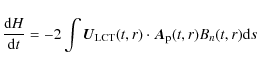
where
In order to locate the EUV filament channel over the photospheric magnetic field configuration we made the co-alignment among H![]() ,
TRACE and MDI data, taking into account the fits header information. We resized the images in H
,
TRACE and MDI data, taking into account the fits header information. We resized the images in H![]() and
at 195 Å to obtain the same pixel resolution of MDI, then we
aligned them considering the latitude and the longitude coordinates of
the field of view centers with respect to the Sun center.
and
at 195 Å to obtain the same pixel resolution of MDI, then we
aligned them considering the latitude and the longitude coordinates of
the field of view centers with respect to the Sun center.
We also performed an extrapolation of the potential magnetic field from a MDI magnetogram using the method of Alissandrakis (1981) to determine the 3D magnetic field configuration in the ARs before the event.
3 Event description
Using H![]() images,
we deduced that the filament involved in the eruption started to form
on Oct. 15, 1999, between two active regions named NOAA 8731
and NOAA 8732 (see the arrow in Fig. 1a). This filament became more visible on 16 Oct. (Fig. 1b)
and assumed an S-shape between 16 and 17 Oct., although the convex
shape of the filament in the southern part is more evident than the
concave shape in the northern part (Fig. 1c). The filament maintained this shape till its eruption (see Fig. 1d) and almost disappeared in H
images,
we deduced that the filament involved in the eruption started to form
on Oct. 15, 1999, between two active regions named NOAA 8731
and NOAA 8732 (see the arrow in Fig. 1a). This filament became more visible on 16 Oct. (Fig. 1b)
and assumed an S-shape between 16 and 17 Oct., although the convex
shape of the filament in the southern part is more evident than the
concave shape in the northern part (Fig. 1c). The filament maintained this shape till its eruption (see Fig. 1d) and almost disappeared in H![]() on Oct. 20. This S-shape of the filament is a first evidence of
the sinistral chirality of the flux rope containing the filament
plasma. In fact, Rust & Martin (1994)
found that filaments with an S-shape usually have their ends curving
toward sunspots with clockwise whirls, and concluded that filaments
with ends curving toward sunspots with clockwise whirls are generally
sinistral.
on Oct. 20. This S-shape of the filament is a first evidence of
the sinistral chirality of the flux rope containing the filament
plasma. In fact, Rust & Martin (1994)
found that filaments with an S-shape usually have their ends curving
toward sunspots with clockwise whirls, and concluded that filaments
with ends curving toward sunspots with clockwise whirls are generally
sinistral.
In Fig. 2a we can see the active regions in white light as observed by TRACE. In Fig. 2b
we overplotted the contours of the magnetic field measured by MDI
(positive in blue and negative in red) on a 195 Å image taken
by TRACE at 5:47 UT on Oct. 20. We see that the EUV filament
channel corresponding to the H![]() filament lies along the neutral line formed by the two active regions
and its footpoints seem to connect the eastern negative polarity of
NOAA 8732 to the western positive polarity of NOAA 8731.
Therefore, the filament seems to show an orientation in accordance with
the solar cycle. In fact, in odd-numbered cycles the magnetic field
vectors point eastward in the northern hemisphere, and vice-versa
(Leroy 1989).
filament lies along the neutral line formed by the two active regions
and its footpoints seem to connect the eastern negative polarity of
NOAA 8732 to the western positive polarity of NOAA 8731.
Therefore, the filament seems to show an orientation in accordance with
the solar cycle. In fact, in odd-numbered cycles the magnetic field
vectors point eastward in the northern hemisphere, and vice-versa
(Leroy 1989).
Following Martin et al. (1994) and Aulanier & Demoulin (1998), we recall that the handedness of the filaments is inherent to the configuration of their fine structure, which can be detected also from bundles of fine structures, as the barbs. In our case (see the arrow in Fig. 1c), the barb curves from the long axis of the filament to the left, providing a further evidence of the sinistral chirality of this filament.
The filament started to activate at 5:50 UT. At the beginning of the eruption the filament was divided into two parts, one remaining in site and another erupting (see Fig. 2c and TRACE movie).
During its eruption the EUV filament channel showed a bundle of helically twisted threads (see the enlarged image at the left low corner of Fig. 2d). This is typical of filament eruptions observed at EUV wavelengths, where portions of the filament appear in emission as a result of localized heating and relevant energy transport along the field lines. Following Chae (2000), this mixture of bright and dark threads makes it possible to discern overlying and underlying threads and to determine the magnetic helicity of the filament. A careful inspection of the movie reveals that during its eruption the filament showed several dark threads interposed by less dark regions. In the insert shown in Fig. 2d we show a more contrasted image of those dark threads (indicated by arrows) with the interposed brighter threads as they appeared at 06:04 UT. The interposition of the dark and bright threads in the image forms a crossing of the type I showed in Fig. 1 of Chae (2000), which indicates positive helicity.
During the main phase of the flare, the ribbons moving away at both sides of the initial filament location appeared (Fig. 2e.)
![\begin{figure}
\par\includegraphics[width=6.1cm]{12425f3.ps}\\\end{figure}](/articles/aa/full_html/2009/41/aa12425-09/img15.png) |
Figure 3:
Top view of the potential field extrapolation obtained from MDI
magnetogram taken on Oct. 19 at 7:59 UT. The field of view is
|
| Open with DEXTER | |
![\begin{figure}
\par\includegraphics[width=6cm,clip]{12425f4a.ps}\\
\hspace*{2....
...aphics[width=6cm,clip]{12425f4c.ps}\\
\hspace*{2.8cm}{\bf (c)}\end{figure}](/articles/aa/full_html/2009/41/aa12425-09/img16.png) |
Figure 4:
a) Map of the helicity transport rate measured at
16:03 UT on Oct. 19. The white line indicates the filament
location; b) contours of the helicity transport rate
measured along the filament at 16:03 UT on Oct. 19, 1999,
overplotted on the H |
| Open with DEXTER | |
The potential field extrapolation performed using the code based on Alissandrakis (1981) method (Fig. 3) on a magnetogram taken on Oct. 19 at 7:59 UT shows that the shape of the potential field lines around the filament location and linking NOAA 8732 and NOAA 8731 is very similar to the post flare loops observed at 195 Å (Fig. 2f). Therefore, we cannot deduce any magnetic helicity sign from the shape of the post flare loop arcade, because it seems to be due to the bending of the photospheric inversion line instead of a real shear of the loop footpoints. Figure 3 allows us also to explain the brightenings present in the eastern part of Fig. 2d probably due to plasma heating in response to downward flux of energetic electrons from the reconnection sites along the eastern footpoints of the main arcade of the active region NOAA 8731.
It is also worth of note that during the eruption the filament apex shows a small rotation. As we can see from the angle formed between the orientation of the ribbons (corresponding to the initial orientation of the filament) and the main axis of the filament plasma at 6:11 UT (see the enlarged image at the left low corner of Fig. 2e), it seems that the filament rotates counterclockwise of about 10 degrees. Although this small rotation should be consistent with negative helicity, as pointed out by Green et al. (2007), the strong projection effects due to the location of the event does not allow us to be confident about this helicity signature.
4 Results
In order to better understand the contribution of the magnetic
helicity to the evolution of the magnetic configuration of the
filament, we applied the Chae's method to the MDI data sets. From the
map of Fig. 4a
we can see that the region is characterized by a highly structured
distribution of the helicity sign, as typically obtained using the
vector potential in the helicity rate computation. However, we note
that along the filament a prevalently positive contribution to the
transport of the magnetic helicity was concentrated around the filament
footpoints. This is also clearly shown in Fig. 4b, where the contours of the positive helicity transport rate are overplotted on a H![]() image. Therefore, we decided to restrict our analysis of the magnetic helicity transport to a neighbouring area of
image. Therefore, we decided to restrict our analysis of the magnetic helicity transport to a neighbouring area of
![]() arcsec2 for both footpoints (indicated by the boxes in Fig. 4c and named 1 and 2).
arcsec2 for both footpoints (indicated by the boxes in Fig. 4c and named 1 and 2).
![\begin{figure}
\par\mbox{\includegraphics[width=9.0cm]{12425f5a.ps}\includegraph...
...12425f5b.ps} }\\
\hspace*{4.5cm}{\bf (a)}\hspace*{8.0cm}{\bf (b)}\end{figure}](/articles/aa/full_html/2009/41/aa12425-09/img18.png) |
Figure 5: Value of the magnetic flux vs. time a) and of the magnetic helicity transport rate vs. time b) of the areas around the footpoint locations 1. In a) thick and thin lines indicate negative and positive flux, respectively. |
| Open with DEXTER | |
![\begin{figure}
\par\mbox{\includegraphics[width=9.0cm]{12425f6a.ps} \includegrap...
...425f6b.ps} }\\
\hspace*{4.5cm}{\bf (a)}\hspace*{8.0cm}{\bf (b)}\end{figure}](/articles/aa/full_html/2009/41/aa12425-09/img19.png) |
Figure 6: Value of the magnetic flux vs. time a) and of the magnetic helicity transport rate vs. time b) of the areas around the footpoint locations 2. In a) thick and thin lines indicate negative and positive flux, respectively. |
| Open with DEXTER | |
As we can see in Figs. 5a and 6a the magnetic flux in these areas is of the order of 1020 to 1021 Mx. In particular, during our observations, we noted an increase of the positive and negative magnetic flux in footpoints 1 and 2, respectively.
The temporal variation in the magnetic helicity transport rate in the
north-east and south-west ends showed an amplitude of the noise of
about
![]() Mx2 h-1 and
Mx2 h-1 and
![]() Mx2 h-1, respectively. This kind of amplitude fluctuation was also noticed in previous studies (Chae 2001,
2004) and was attributed not only to noise, but also to intrinsic
variations associated with surface convective flows. Taking into
account that the use of full-disk magnetograms could also provide
non-negligible effects in the application of the LCT and in order to
have information about the helicity transport rate on long temporal
intervals, we show in Figs. 5b and 6b a smooth of the signal over 0.5 days.
Mx2 h-1, respectively. This kind of amplitude fluctuation was also noticed in previous studies (Chae 2001,
2004) and was attributed not only to noise, but also to intrinsic
variations associated with surface convective flows. Taking into
account that the use of full-disk magnetograms could also provide
non-negligible effects in the application of the LCT and in order to
have information about the helicity transport rate on long temporal
intervals, we show in Figs. 5b and 6b a smooth of the signal over 0.5 days.
In both footpoints we registered a first significant increase of the
positive helicity between 16 and 17 Oct., i.e. when the filament
assumed an S-shape (see Fig. 1c).
Then, on Oct. 17 the helicity transport rate remained positive and
decreased in both footpoints, although the magnetic flux continued to
increase. From about 00:00 UT on 18 Oct. till the end of our
observations, more and more positive magnetic helicity is transported
from the filament ends reaching
![]() and
and
![]() Mx2 h-1 in 1 and 2, respectively.
Mx2 h-1 in 1 and 2, respectively.
5 Conclusions
We have analyzed the evolution of a filament, which appeared on the solar disk on Oct. 15, 1999, and erupted on Oct. 20 during a flare observed by TRACE at 195 Å, between 5:50 and 6:50 UT.
Due to the availability of high resolution data we have reported several signatures providing information on the chirality and the helicity sign of the flux rope containing the filament material: its forward S shape and the orientation of the barbs indicate that the filament chirality was sinistral, while the filament threads observed at 195 Å indicate that the magnetic helicity was positive. The only signature consistent with negative helicity (Green et al. 2007) is a small counterclokwise rotation of the filament apex, but the strong projection effects due to the location of the event does not allow us to be confident about this helicity signature.
Therefore our results allowed us to confirm a correspondence between a sinistral filament and positive magnetic helicity. This correspondence was already deduced by Rust (1999) and by Chae(2000): the former associating the predominance of negative helical magnetic clouds in the northern hemisphere (Bothmer & Schwenn 1994) with the predominance of dextral filaments in the same hemisphere (Martin et al. 1994), the latter through the study of some cases of filaments displaying bright and dark threads in the EUV images taken by TRACE. The same correspondence is also supported by the flux rope model developed by Rust & Kumar (1994) for filaments in which a filament's morphology depends on whether it is formed by magnetic flux with right-handed or left-handed magnetic helicity. Instead, it is in disagreement with the proposition of Martin & McAllister (1997), who argued that when a filament erupts, its barbs are detached from their photospheric roots and the filament develops a left-helical structure when the filament is sinistral, according to the helicity sign of the overlying coronal arcade.
In this study we also measured the magnetic helicity transport
rate at the filament footpoints from its formation to its eruption. We
observed similar and contemporary variations of the helicity transport
rate in both footpoints (although with a different order of magnitude),
which confirms the link between them. In particular, we noted a first
strong increase of the positive magnetic helicity transport rate in
both footpoints just before the filament assumed an S-shape
configuration in H![]() .
A further and continuous increase of the positive magnetic helicity has
been observed until the end of our observations, i.e. few hours before
the eruption of the filament. From the measure of the magnetic flux, it
seems that this helicity transport could be due to the emergence of new
flux from the convection zone.
.
A further and continuous increase of the positive magnetic helicity has
been observed until the end of our observations, i.e. few hours before
the eruption of the filament. From the measure of the magnetic flux, it
seems that this helicity transport could be due to the emergence of new
flux from the convection zone.
This behaviour of the magnetic helicity transport suggests that the photospheric regions where the filament is rooted might be the preferential ways where the magnetic helicity is injected along the filament itself during its formation phase and where the magnetic field configuration is modified.
Therefore this study shows that the magnetic helicity injection measured at filament footpoints could be an important tool to determine the variation of the magnetic configuration (chirality) of the filament flux rope and might be useful to determine the conditions able to trigger an eruption.
AcknowledgementsThe authors wish to thank the anonymous referee for his/her comments and suggestions which led to a sounder version of the manuscript. The authors are grateful to the Global High Resolution HNetwork,operated by Big Bear Solar Observatory, to SOHO/MDI team and to TRACE team for the provision of data. This work was supported by the European Commission through the SOLAIRE Network (MTRN-CT-2006-035484), by the Istituto Nazionale di Astrofisica (INAF), by the Agenzia Spaziale Italiana (contract I/015/07/0) and by the Università degli Studi di Catania.
References
- Alissandrakis, C. E. 1981, A&A, 100, 197 [NASA ADS]
- Aulanier, G., & Demoulin, P. 1998, A&A, 329, 1125 [NASA ADS]
- Aulanier, G., & Demoulin, P. 2003, A&A, 402, 769 [NASA ADS] [CrossRef] [EDP Sciences]
- Aulanier, G., Demoulin, P., van Driel-Gesztelyi, L., Mein, P., & Deforest, C. 1998, A&A, 335, 309 [NASA ADS]
- Berger, M. A., & Field, G. B. 1984, J. Fluid Mech., 147, 133 [NASA ADS] [CrossRef]
- Bothmer, V., & Schwenn, R. 1994, Space Sci. Rev., 70, 215 [NASA ADS] [CrossRef]
- Chae, J. 2000, ApJ, 540, L115 [NASA ADS] [CrossRef]
- Chae, J. 2001, ApJ, 560, L95 [NASA ADS] [CrossRef]
- Demoulin, P. 2007, Adv. Space Res., 39, 1674 [NASA ADS] [CrossRef]
- Demoulin, P., & Pariat, E. 2009, Adv. Space Res., 43, 1013 [NASA ADS] [CrossRef]
- DeVore, C. R., & Antiochos, S. K. 2000, ApJ, 539, 954 [NASA ADS] [CrossRef]
- Leroy, J. L. 1989, Dynamics and structure of quiescent solar prominence, ed. E. R. Priest (Dordrecht: Kluwer), 77
- Martin, S. F., Marquette, B., & Bilimoria, R. 1992, Proc. 12th Summer Workshop, The Solar Cycle, ed. K. Harvey (Sunspot: NSO), 53
- Martin, S. F., Bilimoria, R., & Tracadas, P. W. 1994, Solar Surface Magnetism, ed. R. J. Rutten, C. J. Schrijver (Dordrecht: Kluwer Acad. Publ.), 303
- Martin, S. F., & Echols, C. R. 1994, Solar Surface Magnetism, ed. R. J. Rutten, & C. J. Schrijver (Dordrecht, Holland: Kluwer Academic Publishers), 339
- Martin, S. F., & McAllister, A. H. 1997, in Coronal Mass Ejections, ed. N. Crooker, J. Joselyn, & J. Feynman, Geophys. Monogr. 111, Washington, DC, AGU, 127
- November, L. J., & Simon, G. W. 1988, ApJ, 333, 427 [NASA ADS] [CrossRef]
- Romano, P., Contarino, L., & Zuccarello, F. 2003, Sol. Phys., 214, 313 [NASA ADS] [CrossRef]
- Rust, D. M., & Kumar, A. 1994, ESA SP-373, 39
- Rust, D. M., & Kumar, A. 1996, ApJ, 464, L199 [NASA ADS] [CrossRef]
- Rust, D. M., & Martin, S. 1994, Solar Active Region Evolution: Comparing Models with Observations, ed. K. S. Balasubramaniam, & G. W. Simon, ASP Conf. Ser. San Francisco, 68, 337
- Schrijver, C. J. 2009, Adv. Space Res., 43, 739 [NASA ADS] [CrossRef]
- van Ballegooijen, A. A. 2004, ApJ, 612, 519 [NASA ADS] [CrossRef]
All Figures
| |
Figure 1:
Sequence of H |
| Open with DEXTER | |
| In the text | |
| |
Figure 2:
a) TRACE image taken in white light showing the photospheric configuration of NOAA 8731 and NOAA 8732; b) contours
of the magnetic field measured by MDI on a 195 Å image taken
by TRACE; the contour levels (red indicates the negative polarity and
blue indicates the positive polarity) correspond to |
| Open with DEXTER | |
| In the text | |
| |
Figure 3:
Top view of the potential field extrapolation obtained from MDI
magnetogram taken on Oct. 19 at 7:59 UT. The field of view is
|
| Open with DEXTER | |
| In the text | |
| |
Figure 4:
a) Map of the helicity transport rate measured at
16:03 UT on Oct. 19. The white line indicates the filament
location; b) contours of the helicity transport rate
measured along the filament at 16:03 UT on Oct. 19, 1999,
overplotted on the H |
| Open with DEXTER | |
| In the text | |
| |
Figure 5: Value of the magnetic flux vs. time a) and of the magnetic helicity transport rate vs. time b) of the areas around the footpoint locations 1. In a) thick and thin lines indicate negative and positive flux, respectively. |
| Open with DEXTER | |
| In the text | |
| |
Figure 6: Value of the magnetic flux vs. time a) and of the magnetic helicity transport rate vs. time b) of the areas around the footpoint locations 2. In a) thick and thin lines indicate negative and positive flux, respectively. |
| Open with DEXTER | |
| In the text | |
Copyright ESO 2009
Current usage metrics show cumulative count of Article Views (full-text article views including HTML views, PDF and ePub downloads, according to the available data) and Abstracts Views on Vision4Press platform.
Data correspond to usage on the plateform after 2015. The current usage metrics is available 48-96 hours after online publication and is updated daily on week days.
Initial download of the metrics may take a while.