Planet migration in three-dimensional radiative discs

W. Kley; B. Bitsch; H. Klahr

doi:10.1051/0004-6361/200912072

Home

All issues

Volume 506 / No 2 (November I 2009)

A&A, 506 2 (2009) 971-987

Full HTML

Highlight

Free Access

Issue		A&A Volume 506, Number 2, November I 2009


Page(s)		971 - 987
Section		Planets and planetary systems
DOI		https://doi.org/10.1051/0004-6361/200912072
Published online		27 August 2009

A&A 506, 971-987 (2009)

Planet migration in three-dimensional radiative discs

W. Kley¹ - B. Bitsch¹ - H. Klahr²

1 - Institut für Astronomie & Astrophysik, Universität Tübingen, Auf der Morgenstelle 10, 72076 Tübingen, Germany
2 - Max-Planck-Institut für Astronomie, Heidelberg, Germany

Received 15 March 2009 / Accepted 10 August 2009

Abstract
Context. The migration of growing protoplanets depends on the thermodynamics of the ambient disc. Standard modelling, using locally isothermal discs, indicate an inward (type-I) migration in the low planet mass regime. Taking non-isothermal effects into account, recent studies have shown that the direction of the type-I migration can change from inward to outward.
Aims. In this paper we extend previous two-dimensional studies and investigate the planet-disc interaction in viscous, radiative discs using fully three-dimensional radiation hydrodynamical simulations of protoplanetary accretion discs with embedded planets, for a range of planetary masses.
Methods. We use an explicit three-dimensional (3D) hydrodynamical code NIRVANA that includes full tensor viscosity. We have added implicit radiation transport in the flux-limited diffusion approximation, and to speed up the simulations significantly we have newly adapted and implemented the FARGO-algorithm in a 3D context.
Results. First, we present results of test simulations that demonstrate the accuracy of the newly implemented FARGO-method in 3D. For a planet mass of 20 $M_{\rm earth}$ , we then show that including radiative effects also yields a torque reversal in full 3D. For the same opacity law, the effect is even stronger in 3D than in the corresponding 2D simulations, due to a slightly thinner disc. Finally, we demonstrate the extent of the torque reversal by calculating a sequence of planet masses.
Conclusions. Through full 3D simulations of embedded planets in viscous, radiative discs, we confirm that the migration can be directed outwards up to planet masses of about 33 $M_{\rm earth}$ . As a result, the effect may help to resolve the problem of inward migration of planets that is too rapid during their type-I phase.

Key words: accretion, accretion disks - hydrodynamics - radiative transfer - planets and satellites: formation

1 Introduction

The process of migration in protoplanetary discs allows forming planets to move away from the location of creation and finally end up at a different position. The cause of this change in distance from the star are the tidal torques acting from the disturbed disc back on the protoplanet. These can be separated into two parts: i) the so-called Lindblad torques that are created by the two spiral arms in the disc and ii) the corotation torques that are caused by the co-orbital material as it periodically exchanges angular momentum with the planet on its horseshoe orbit. For comprehensive introductions to the field, see for example Papaloizou et al. (2007) or Masset (2008), and references therein. The Lindblad torques, caused by density waves launched at Lindblad resonances, quite generally lead to an inward motion of the planet explaining the observed hot planets very nicely (Ward 1997). The corotation torques are mainly caused by two effects, first by a gradient in the vortensity (Tanaka et al. 2002) and second by a gradient in the entropy (Baruteau & Masset 2008). For typical protoplanetary discs, both contributions can be positive, possibly counterbalancing the negative Lindblad torques (Paardekooper & Mellema 2006; Baruteau & Masset 2008). For the typically considered locally isothermal discs where the temperature only depends on the radial distance from the star, the net torque is negative, and migration is directed inwards for typical disc parameters (Tanaka et al. 2002). Through planetary synthesis models, the inferred rapid inward migration of planetary cores has been found to be inconsistent with the observed mass-distance distribution of exoplanets (Alibert et al. 2004; Ida & Lin 2008). Possible remedies are the retention of icy cores at the snow line or a strong reduction in the speed of type-I migration (of embedded low-mass planets). Here we focus on the latter process.

Different mechanisms for slowing down the too rapid inward migration have been discussed (Li et al. 2009; Masset et al. 2006), but including more realistic physics seems to be particularly appealing. As pointed out first by Paardekooper & Mellema (2006), the inclusion of radiative transfer can cause a strong reduction in the migration speed. The process has been subsequently investigated by several groups (Kley & Crida 2008; Paardekooper & Mellema 2008; Paardekooper & Papaloizou 2008; Baruteau & Masset 2008), who show that the migration process can indeed be slowed down or even reversed for sufficiently low-mass planets. This new effect occurs in non-isothermal discs and scales with the gradient of the entropy (Baruteau & Masset 2008), hence entropy-related torque. However, in a strictly adiabatic situation after a few libration time scales, the entropy gradient will flatten within the corotation region due to phase mixing. This will lead to saturation (and subsequent disappearance) of the part of the corotation torque that is caused by the entropy gradient in the horseshoe region (Paardekooper & Papaloizou 2009; Baruteau & Masset 2008). To prevent saturation of this entropy-related torque, some radiative diffusion (or local radiative cooling) is required (Kley & Crida 2008). Since for genuinely inviscid flows, the streamlines in the horseshoe region will be closed and symmetric with respect to the planet's location, some level of viscosity is always necessary to avoid torque saturation (Ogilvie & Lubow 2003; Paardekooper & Papaloizou 2008; Masset 2001; Paardekooper & Papaloizou 2009). This applies to both the vortensity- and entropy-related corotation torques. The maximum planet mass for which a change of migration may occur due to this effect lies for typical disc masses in the range of about 40 earth masses, beyond which the migration rate follows the standard (isothermal) case, as gap formation sets in which reduces the corotation effects (Kley & Crida 2008). Most of the above simulations have studied only the two-dimensional case, while three-dimensional models including radiative effects have been presented only for very low masses (Paardekooper & Mellema 2006), or for Jupiter type planets (Klahr & Kley 2006). A range of planet masses has not yet been studied systematically in full 3D.

In this paper we investigate the planet-disc interaction in radiative discs using fully three-dimensional radiation hydrodynamical simulations of protoplanetary accretion discs with embedded planets for a variety of planetary masses. For that purpose we modified and substantially extended an existing multi-dimensional hydrodynamical code Nirvana (Kley et al. 2001; Ziegler & Yorke 1997a) by incorporating the FARGO-algorithm (Masset 2000a) and radiative transport in the flux-limited diffusion approximation (Levermore & Pomraning 1981; Kley 1989). The code Nirvana can in principle handle nested grids which allows us to zoom-in on the detailed structure in the vicinity of the planet (D'Angelo et al. 2002,2003), however in the present context we limit ourselves to single grid simulations. We present several test cases to demonstrate first the accuracy of the FARGO-method in 3D. We then proceed to analyse the effects of radiative transport on the disc structure and torque balance. For our standard planet of $20~ M_{\rm earth}$ , we find that the effect of torque reversal appears to be even stronger in 3D than in 2D for an otherwise identical physical setup. We have a more detailed look at the implementation of the planet potential and show that it has definitely an influence on the strength of the effect. Finally, we perform simulations for a sequence of different planet masses to evaluate the mass range over which the migration may be reversed. The consequence for the migration process and the overall evolution of planets in discs is discussed.

2 Physical modelling

The protoplanetary disc is treated as a three-dimensional (3D), non-self-gravitating gas whose motion is described by the Navier-Stokes equations. The turbulence in discs is thought to be driven by magneto-hydrodynamical instabilities (Balbus & Hawley 1998). Since we are interested in this study primarily on the average effect the disc has on the planet, we prefer in this work to simplify and treat the disc as a viscous medium. The dissipative effects can then be described via the standard viscous stress-tensor approach (e.g. Mihalas & Weibel Mihalas 1984). We assume that the heating of the disc occurs solely through internal viscous dissipation and ignore in the present study the influence of additional energy sources such as irradiation from the central star or other external sources. The internally produced energy is then radiatively diffused through the disc and eventually emitted from its surfaces. To describe this process we utilise the flux-limited diffusion approximation (FLD, Levermore & Pomraning 1981) which allows to treat approximately the transition from optically thick to thin regions near the disc's surface.

2.1 Basic equations

Discs with embedded planets have mostly been modelled through 2D simulations in which the disc is assumed to be infinitesimal thin, and vertical integrated quantities are used to describe the time evolution of the disc with the embedded planet. This procedure saves considerable computational effort but is naturally not as accurate as truly 3D simulations, in particular the radiation transport is difficult to model in a 2D context.

In this work we present an efficient method for 3D disc simulations based on the FARGO algorithm (Masset 2000a). For accretion discs where material is orbiting a central object the best suited coordinates are spherical polar coordinates $(r, \theta, \varphi)$ where r denotes the radial distance from the origin, $\theta$ the polar angle measured from the z-axis, and $\varphi$ denotes the azimuthal coordinate starting from the x-axis.

In this coordinate system, the mid-plane of the disc coincides with the equator ( $\theta=\pi/2$ ), and the origin of the coordinate system is centred on the star. Sometimes we will need the radial distance from the polar axis which we denote by a lower case s, which is the radial coordinate in cylindrical coordinates.

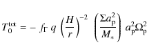
For a better resolution of the flow in the vicinity of the planet, we work in a rotating coordinate system which rotates with the orbital angular velocity $\Omega$ , which is identical to the orbital angular velocity of the planet

$\begin{displaymath}\Omega_P = \left[\frac{G~(M_*+m_{\rm p})}{a^3}\right]^{1/2} \end{displaymath}$

(1)

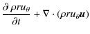
where M_* is the mass of the star, $m_{\rm p}$ the mass of the planet, and athe semi-major axis of the planet. Only for testing purposes for our implementation of the FARGO-method we let the planet move under the action of the disc.

The Navier-Stokes equations in a rotating coordinate system in spherical coordinates read explicitly:

a) Continuity equation

$\begin{displaymath}\frac{\partial ~ \rho}{\partial t} + \nabla \cdot (\rho~ \vec{u}) = 0. \end{displaymath}$

(2)

Here $\rho$ denotes the density of the gas and $\vec{u}=(u_r, u_\theta, u_\varphi)$ its velocity.

b) Radial momentum

$\displaystyle \frac{\partial ~ \rho u_r}{\partial t} + \nabla \cdot (\rho~u_r~\vec{u} )$	=	$\displaystyle \rho \frac{u_\theta^2}{r} + \rho r \sin^2 \theta ~ ( \omega + \Omega)^2$
		$\displaystyle + \rho a_r - \frac{\partial p}{\partial r} - \rho~\frac{\partial \Phi}{\partial r} + f_{\rm\it r}.$	(3)

Here $\omega$ is the azimuthal angular velocity as measured in the rotating frame, p is the gas pressure, and $\Phi$ denotes the gravitational potential due to the star and the planet. The vector $\vec{a}=(a_r, a_\theta, a_\varphi)$ represents inertial forces generated by the accelerated origin of the coordinate system. Specifically, $\vec{a}$ equals the negative acceleration acting on the star due to the planet(s).

c) Meridional momentum

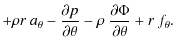
$\displaystyle \frac{\partial ~ \rho r u_\theta}{\partial t} + \nabla \cdot (\rho r u_\theta \vec{u})$	=	$\displaystyle \rho r^2 \sin \theta \cos \theta ~ (\omega + \Omega)^2$
		$\displaystyle + \rho r ~ a_\theta - \frac{\partial p}{\partial \theta} - \rho~ \frac{\partial \Phi}{\partial \theta} + r \ f_{\rm\theta}.$	(4)

d) Angular momentum

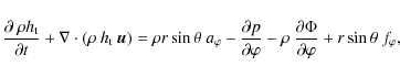
$\begin{displaymath}\frac{\partial ~ \rho h_{\rm t}}{\partial t} + \nabla \cdot \... ...tial \Phi}{\partial \varphi} + r \sin\theta \ f_{\rm\varphi}, \end{displaymath}$

(5)

where we defined the total specific angular momentum (in the inertial frame)

$\begin{displaymath}h_{\rm t} = r^2~ \sin^2 \theta \left( \omega + \Omega \right); \end{displaymath}$

(6)

i.e. the azimuthal velocity in the rotating frame is given by $u_\varphi = \omega~r~ \sin\theta$ .

The Coriolis force in Eq. (5) for $u_\varphi$ (or $h_{\rm t}$ ) has been incorporated into the left hand side. Thus, it is written in such a way as to conserve total angular momentum best. This conservative treatment is necessary to obtain an accurate solution of the embedded planet problem (Kley 1998).

The function $\vec{f} = (f_r, f_\theta, f_\varphi)$ in the momentum equations denotes the viscous forces which are stated explicitly for the three-dimensional case in spherical polar coordinates in Tassoul (1978). For the description of the viscosity we use a constant kinematic viscosity coefficient $\nu$ .

e) Energy equation (internal energy)

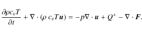
$\begin{displaymath}\frac{\partial \rho c_v T}{\partial t} + \nabla \cdot \left( ... ...ht) = - p \nabla \cdot \vec{u} + Q^+ - \nabla \cdot \vec{F}. \end{displaymath}$

(7)

Here T denotes the gas temperature in the disc and $c_{\rm v}$ is the specific heat at constant volume. On the right hand side, the first term describes compressional heating, Q⁺ the viscous dissipation function, and $\vec{F}$ denotes the radiative flux. In writing Eq. (7) we have assumed that the radiation energy density $E=a_{\rm R} T^4$ is always lower than the thermal energy density $e=\rho c_v T$ . Here, $a_{\rm R}$ denotes the radiation constant. Furthermore, we utilise the one-temperature approach and write for the radiative flux, using flux-limited diffusion (FLD)

$\begin{displaymath} \vec{F} = - \frac{\lambda c ~ 4 a_{\rm R} T^3}{\rho (\kappa + \sigma)} ~ \nabla T\ , \end{displaymath}$

(8)

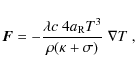
where c is the speed of light, $\kappa$ the Rosseland mean opacity, $\sigma$ the scattering coefficient, and $\lambda$ the flux-limiter. Using FLD allows us to perform stable accretion disc models that cover several vertical scale heights. We use here the FLD approach described in Levermore & Pomraning (1981) with the flux-limiter of Kley (1989). Its suitability for protostellar discs has been shown in Kley & Lin (1999,1996), and for embedded planets in Klahr & Kley (2006). In this work we use for the Rosseland mean opacity $\kappa(\rho, T)$ the analytical formulae by Lin & Papaloizou (1985) and set the scattering coefficient $\sigma$ to zero. To close the basic system of equations we use an ideal gas equation of state where the gas pressure is given by $p= R_{\rm gas} \rho T /\mu$ , with the mean molecular weight $\mu$ and gas constant $R_{\rm gas}$ . For a standard solar mixture we assume here $\mu=2.35$ . The speed of sound is calculated from $c_{\rm s}=\sqrt{\gamma p / \rho}$ with the adiabatic index $\gamma =1.43$ .

$\begin{figure} \par\includegraphics[width=9cm,clip]{12072fg01.eps} \end{figure}$

Figure 1:

The gravitational potential of a $20~ M_{\rm earth}$ planet with different smoothings applied, see Eqs. (9) and (10). The distance d from the planet is given in units of $a_{\rm p}$ (here $a_{\rm Jup}$ ), and the smoothing length $r_{\rm sm}$ in units of the Hill radius of the planet which refers here to $R_{\rm H} = 0.0271 a_{\rm p}$ . Note that the data points are drawn directly from the used 3D computational grid and indicate our standard numerical resolution (see Sect. 2.4).

Open with DEXTER

2.2 Planetary potential

The total potential $\Phi$ acting on the disc consists of two contributions, one from the star $\Phi_*$ , the other from the planet $\Phi_{\rm p}$

$\begin{displaymath}\Phi = ~ \Phi_* + \Phi_{\rm p} ~ = - ~ \frac{G M_*}{r} - \frac{G m_{\rm p}}{\sqrt{(\vec{r}-\vec{r}_{\rm p})^2}}, \end{displaymath}$

where $\vec{r}_{\rm p}$ denotes the radius vector of the planet location. The embedded planet is modelled as a point mass that orbits the central star on a fixed circular orbit. In numerical simulations the planetary potential has to be smoothed over a few gridcells to avoid divergences.

Typically in 2D simulations the planetary potential is modelled by an $\epsilon$ -potential

$\begin{displaymath} \Phi_{\rm p}^{\epsilon} = - \frac{G m_{\rm p}}{\sqrt{d^2 + \epsilon^2}}, \end{displaymath}$

(9)

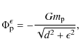
where we denote the distance of the disc element to the planet with $d = \vert\vec{r}-\vec{r}_{\rm p}\vert$ and $\epsilon$ is the smoothing length. In a 2D configuration a potential of this form is indeed very convenient, as the smoothing takes effects of the otherwise neglected vertical extent of the disc into account. To account for the finite disc thickness Hwhich depends on the temperature in the disc, an often used value for the smoothing length in 2D-simulations is $\epsilon = r_{\rm sm} = 0.6 H$ . The obtained 2D torques are then found to be in reasonable agreement with three-dimensional analytical estimates of the torques, that do not include a softening length for the planet potential.

However in a 3D configuration the same approach is not necessary and would lead to an unphysical ``spreading'' of the potential over a large region. Hence, we apply a different type of smoothing, follow Klahr & Kley (2006) and use a cubic-potential of the form

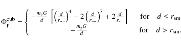
$\begin{displaymath} \Phi_{\rm p}^{\rm cub} = \left\{ \begin{array}{cc} - \fra... ...quad & \mbox{for} \quad d > r_{\rm sm}. \end{array} \right. \end{displaymath}$

(10)

This potential is constructed in such a way as to yield for distances dgreater than $r_{\rm sm}$ the correct 1/r potential of the planet, and inside that radius ( $d < r_{\rm sm}$ ) the potential is smoothed with a cubic polynomial such that at the transition radius $r_{\rm sm}$ the potential and its first and second derivative agree with the analytic outside 1/r-potential. To illustrate the various types of smoothing, we display in Fig. 1 the behaviour of the different forms of the planetary potential. Clearly the $\epsilon$ -potential leads for the same values of $r_{\rm sm}$ to a much wider and shallower potential than our cubic-approach. For the often used value $\epsilon = 0.6 H$ the $\epsilon$ -potential is felt way outside the Hill radius

$\begin{displaymath}R_{\rm H} = a_{\rm p} \left(\frac{m_{\rm p}}{3 ~M_*}\right)^{1/3} , \end{displaymath}$

and leads to a significant underestimate of the potential depth already at $r_{\rm sm}$ . The cubic-potential (Eq. (10)) will always be accurate down to $d = r_{\rm sm}$ and is inside much deeper than the $\epsilon$ -potential, and hence more accurate. In the simulations presented below we study in detail the influence that the potential description has on the value of the torques acting on the planet.

We calculate the gravitational torques acting on the planet by integrating over the whole disc, where we apply a tapering function to exclude the inner parts of the Hill sphere of the planet. Specifically, we use the smooth (Fermi-type) function

$\begin{displaymath} f_b (d)=\left[\exp\left(-\frac{d/R_H-b}{b/10}\right)+1\right]^{-1} \end{displaymath}$

(11)

which increases from 0 at the planet location (d=0) to 1 outside $d \geq R_{H}$ with a midpoint f_b = 1/2 at d = b R_H, i.e. the quantity b denotes the torque-cutoff radius in units of the Hill radius. This torque cutoff is necessary to avoid first a large, possibly very noisy contribution from the inner parts of the Roche lobe, and second to disregard material that is gravitationally bound to the planet. The question of torque cutoff and exclusion of Roche lobe material becomes very important when i) the disc self-gravity is neglected, and ii) there exists material bound to the planet (e.g. a circumplanetary disc). This issue should definitely be addressed in the future. Here, we assume a transition radius of b = 0.8 Hill radii (see Crida et al. 2008, Fig. 2). For reference we quote the width of the horseshoe region which is given for an isothermal disc approximately by (Masset et al. 2006)

$\begin{displaymath} x_{\rm s} = 1.16 ~ a_{\rm p} ~ \sqrt{\frac{q}{(H/r)}} \end{displaymath}$

(12)

with the mass ratio $q = m_{\rm p}/M_*$ and the local relative disc thickness H/r. For an adiabatic disc H has to be replaced by $\gamma H$ (Baruteau & Masset 2008).

2.3 Setup

The three-dimensional ( $r, \theta, \varphi$ ) computational domain consists of a complete annulus of the protoplanetary disc centred on the star, extending from $r_{\rm min} = 0.4$ to $r_{\rm max} = 2.5$ in units of $r_0 = a_{\rm Jup} = 5.2$ AU. In the vertical direction the annulus extends from the disc's midplane (at $\theta = 90^\circ$ ) to about $7^\circ$ (or $\theta = 83^\circ$ ) above the midplane. In case of an inclined planet the domain has to be extended and cover the upper and lower half of the disc. The mass of the central star is one solar mass $M_* = M_\odot$ , and the total disc mass inside $[r_{\rm min},r_{\rm max}]$ is $M_{\rm disc} = 0.01 ~M_\odot$ . For the present study, we use a constant kinematic viscosity coefficient with a value of $\nu = 10^{15}$ cm²/s, a value that relates to an equivalent $\alpha = 0.004$ at r₀ for a disc aspect ratio of H/r = 0.05, where $\nu = \alpha H^2 \Omega_K$ . In standard dimensionless units we have $\nu = 10^{-5}$ .

The models are initialised with a locally isothermal configuration where the temperature is constant on cylinders and has the profile $T(s) \propto s^{-1}$ , where s is related to r through $s = r \sin \theta$ . This yields a constant ratio of the disc's vertical height H to the radius s. The initial vertical density stratification is approximately given by a Gaussian:

$\begin{displaymath}\rho(r,\theta)= \rho_0 (r) ~ \exp \left[ - \frac{(\pi/2 - \theta)^2 ~ r^2}{2 H^2} \right]\cdot \end{displaymath}$

(13)

Here, the density in the midplane is $\rho_0 (r) \propto r^{-1.5}$ which leads to a $\Sigma(r) \propto ~ r^{-1/2}$ profile of the vertically integrated surface density. The vertical and radial velocities, $u_\theta$ and u_r, are initialised to zero. The initial azimuthal velocity $u_\varphi$ is given by the equilibrium of gravity, centrifugal acceleration and the radial pressure gradient. In case of purely isothermal calculations this setup is equal to the equilibrium configuration (in the case of closed radial boundaries). For fully radiative simulations the model is first run in a 2D axisymmetric mode to obtain a new self-consistent equilibrium where viscous heating balances radiative transport/cooling from the surfaces (see Sect. 4.1 below). This initialisation through an axisymmetric 2D phase (in the $r-\theta$ plane) reduces the required computational effort substantially, as the evolution from the initial isothermal state towards the radiative equilibrium takes about 100 orbits, if the disc is started with an isothermal equilibrium having constant H/r. After reaching the equilibrium between viscous heating and radiative transport/cooling, we extend this model to a full 3D simulation, by expanding the grid into the $\phi$ -direction, and the planet is embedded.

$\begin{figure} \par\includegraphics[width=9cm,clip]{12072fg2a.eps}\par\includegr... ...{12072fg2b.eps}\par\includegraphics[width=9cm,clip]{12072fg2c.eps} \end{figure}$	Figure 2: Evolution of semi-major axis, eccentricity and inclination as a function of time for a 20 $M_{\rm earth}$ planet in a three-dimensional disc. Results are displayed for different numerical resolutions ( $N_r, N_\theta , N_\varphi$ ), and using Fargo and Non-Fargo runs.
Open with DEXTER

2.4 Numerics

We adopt a coordinate system, which rotates at the orbital frequency of the planet. For our standard cases, we use an equidistant grid in $r, \theta, \varphi$ with a resolution of $(N_r,N_\theta, N_\varphi) = (266,32,768)$ . To minimise disturbances (wave reflections) from the radial boundaries, we impose, at $r_{\rm min}$ and $r_{\rm max}$ , damping boundary conditions where all three velocity components are relaxed towards their initial state on a timescale of approximately the local orbital period. The radial velocities at the inner and outer radius vanish. The angular velocity is relaxed towards the Keplerian values. For the density and temperature, we apply reflective radial boundary conditions. In the azimuthal direction, periodic boundary conditions are imposed for all variables. In the vertical direction we apply outflow boundary conditions. The boundary conditions do not allow for mass accretion through the disc, such that the total disc mass remains nearly constant during the time evolution, despite a possible small change due to little outflow through the vertical boundaries and the used density floor (see below).

The numerical details of the used finite volume code (NIRVANA) relevant for these planet disc simulations were described in Kley et al. (2001) and D'Angelo et al. (2003). In the latter paper the usage of the nested grid-technique is described in more detail as well. The original version of the NIRVANA code, on which our programme is based upon, has been developed by Ziegler & Yorke (1997b). The empowerment with FARGO is based on the original work by Masset (2000a). Our implementation appears to be the first inclusion of the FARGO-algorithm in a 3D spherical coordinate system. More details about the implementation are given in the appendix. The basic algorithm of the newly implemented radiation part in the energy Eq. (7) is presented in the appendix as well. To avoid possible time step limitations this part is always solved implicitly.

3 Test calculations

3.1 The `FARGO`-algorithm

To test the 3D implementation of the FARGO-algorithm in our NIRVANA-code we have run several models with planets on circular, elliptic and inclined orbits with and without the FARGO-method applied. Here, we follow closely the models presented in Cresswell et al. (2007) and consider moving planets in 3D discs. As the tests are dynamically already complicated we use here only the isothermal setup. The different setups gave very similar results in all cases, and we present results for one combined case of a 20 $M_{\rm earth}$ planet embedded in a locally isothermal disc with an initial non-zero eccentricity (e=0.2) and non-zero inclination ( $i=5^\circ$ ). All physical parameters of this run are identical to those described in Cresswell et al. (2007), and we compare our results to the last models presented in that paper (their Fig. 16). The outcome of this comparison is shown in Fig. 2, where we display the results of a standard non-Fargo run with the resolution $(N_r,N_\theta, N_\phi)= (264,80,800)$ with the data taken from Cresswell et al. (2007) (where a different code has been used) to two runs having a lower resolution of $(N_r,N_\theta, N_\varphi) = (128,34,384)$ , one with FARGO and the other one without. We can see that all 3 models (obtained with two different codes, methods and resolutions) yield very similar results. The scatter of the data points is slightly reduced in the FARGO-run.

$\begin{figure} \par\includegraphics[width=4.4cm,clip]{12072fg3a.eps}\hspace*{1.5mm} \includegraphics[width=4.4cm,clip]{12072fg3b.eps} \end{figure}$	Figure 3: Radial stratification of surface density ( left) and the midplane temperature ( right) in the disc. This dashed lines represent simple approximations to the 3D stratified results. The solid (green) curves labelled ``flat'' refer to corresponding results for a vertically integrated flat 2D disc using the same input physics.
Open with DEXTER

$\begin{figure} \par\includegraphics[width=4.4cm,clip]{12072fg4a.eps}\hspace*{1.5mm} \includegraphics[width=4.4cm,clip]{12072fg4b.eps} \end{figure}$	Figure 4: Vertical stratification of density ( left) and temperature ( right) at a radius of r=1.44. Thin dashed lines just represent simple functional relations.
Open with DEXTER

3.2 The radiation algorithm

To obtain an independent test of the newly implemented radiation transport module in our NIRVANA-code we performed a run with the standard setup as described above but with no embedded planet. Hence, this setup refers to an axisymmetric disc with internal heating and radiative cooling. For a fixed, closed computational domain it is only the total mass enclosed that determines the final equilibrium state of the system, once the physics (viscosity, opacity, and equation of state) have been prescribed. The radial dependence of the vertically integrated surface density and the midplane temperature are displayed in Fig. 3, and the corresponding vertical profiles at a radius of r=1.44 in Fig. 4. First of all, these new results obtained with NIRVANA agree very well with those obtained with the completely independent 2D-code RH2D used in the $r-\theta$ mode, such as presented for example in Kley et al. (1993), which are not shown in the figures, however. As the final configuration of the system is given by the equilibrium of internal (viscous) dissipation and radiative transport, this test demonstrates the consistency of our implementations.

To relate our 3D results to previous radiative 2D runs which use vertically integrated quantities, and hence can only use an approximative energy transport and cooling (Kley & Crida 2008), we compare in Fig. 3 the results obtained with the two methods. Both models are constructed for the same disc mass and identical physics. The label ``flat'' in the figure refers to the flat 2D case (obtained with RH2D, see Kley & Crida 2008) and the ``stratified'' label to our new 3D implementation presented here. The left graph displays the vertically integrated surface density distribution, here $\Sigma(r) = f_\Sigma \int_{\theta_{\rm max}}^{\theta_{\rm min}} \rho r \sin(\theta) {\rm d}\theta$ , with $f_\Sigma = 1$ for two-sided and 2 for one-sided discs. Our result is well represented by a $\Sigma \propto r^{-1/2}$ profile as expected for a closed domain and constant viscosity. Interesting is the irregular structure at radii smaller than $r\approx 1.0$ in the full 3D stratified case, and we point out that these refer to the onset of convection inside that radius. To model convection is of course not possible in a flat 2D approach. The temperature distribution for the full 3D case follows approximately a $T \propto r^{-1.7}$ profile. Here, the approximate flat-disc model leads to midplane temperatures that are about 40% higher for the bulk part of the domain than in the true 3D case. Possibly a refined modelling of the vertical averaging procedure and the radiative losses in the flat 2D case could improve the agreement here, but in the presence of convection we may expect differences in any case.

In Fig. 4 we display the vertical stratification of the disc at a specific radius in the middle of the computational domain at r=1.44. Two simple approximations are over-plotted as dashed lines. Note, that in these plots the stratification is plotted along the $r={\rm const}.$ lines which deviates for thin discs only slightly from $z = r \cos \theta$ . Taking z₀=0.08, the Gaussian curve for the density refers to $\rho_0 \exp\left[-(z/z_0)^2\right]$ and the temperature fit to T(z) = T₀ [ 1 - 0.4 (z/z₀)²]. These simple formulae are intended to guide the eye rather than meant to model exactly the structure at this radius which depends on the used opacities. Given the simplicity of these, it is interesting that they approximate the true solution reasonably well within one scale height.

3.3 Density floor

By expanding the computed area in the $\theta$ -direction beyond the $90^\circ$ to $83^\circ$ region of our standard model, the code would have to cover several orders of magnitude in the density. Thus, many more grid cells would be required to resolve the physical quantities. In order to avoid this and save computation time, we apply a minimum density function (floor) for the low-density regions high above the equatorial plane of the disc. It reads

$\begin{displaymath}\rho = \left\lbrace \begin{array}{cc} \rho & \quad \mbox{for... ...mbox{for} \quad \rho \le \rho_{\rm min}. \end{array} \right. \end{displaymath}$

(14)

Of course, applying a density floor like this will create mass inside the computed domain. The density floor $\rho_{\rm min}$ has now to be chosen such that: firstly the computation is not handicapped by too low values and secondly the inner (optically thick) parts of the disc are not influenced. To test the sensitivity of the disc structure against the density floor we performed a series of test calculations, and show the results of simulations with different $\rho_{\rm min}$ in Fig. 5. These runs cover $\theta = 90^\circ$ to $70^\circ$ , a range about 3 times as large as before. The density and temperature profiles in these simulations do not differ for the regions near the equatorial plane, because the density is too high for the minimum density to take effect. Indeed, all curves are nearly indistinguishable in the region for optical depths greater than $\tau =1.0$ , with

$\begin{displaymath}\tau(z) = \int_z^\infty \rho \kappa {\rm d}z. \end{displaymath}$

(15)

Please note, that in the plot we do display the results along lines of constant (spherical) radius. Moving further away from the equatorial plane, one can see in the density profile the different minimum densities, but in the temperature profile there is hardly any difference at all. Above a certain distance from the equatorial plane the temperature remains constant. The little fluctuations visible in the profile are due to oscillations in the temperature for the low mass regions.

$\begin{figure} \par\includegraphics[width=8cm,clip]{12072fg5a.eps} \includegraphics[width=8cm,clip]{12072fg5b.eps} \end{figure}$	Figure 5: Vertical stratification of density in logarithmic scale ( top) and temperature ( bottom) at a radius of r=1.00 for a simulation covering the $\theta = 90^\circ$ to $70^\circ$ region. The optical depth $\tau =1.0$ is reached at about z=0.055.
Open with DEXTER

By applying a minimum density the code is capable of resolving large distances above the equatorial plane with a reasonable number of grid cells. Also note that it is not necessary to use a minimum density for calculations covering only the $\theta = 90^\circ$ to $83^\circ$ regions, as the density is always high enough.

4 Models with an embedded planet

For all the models with embedded planets we use our standard disc setup as described in Sect. 2.3 with the corresponding boundary conditions in Sect. 2.4. Here, we briefly summarise some important parameter of the setup. The three-dimensional ( $r, \theta, \varphi$ ) structure of the disc extends form $r_{\rm min} = 0.4$ to $r_{\rm max} = 2.5$ in units of $r_0 = a_{\rm Jup} = 5.2$ AU. In the vertical direction the annulus extends from the disc's midplane (at $\theta = 90^\circ$ ) to about $7^\circ$ (or $\theta = 83^\circ$ ) above the midplane. For our chosen grid size of $(N_r, N_\varphi, N_\theta) = (266, 32, 768)$ this refers to linear grid resolution of $\Delta \approx 0.008$ at the location of the planet, which corresponds to 3.3 gridcells per Hill radius, and to about 5 gridcells per horseshoe half-width for a $20~ M_{\rm earth}$ planet in a disc with H/r =0.05. In this configuration the planet is located exactly at the corner of a gridcell. In the fully radiative disc, the temperature at the disc surface is kept at the fixed ambient temperature of 10 K. This simple ``low-temperature'' boundary condition ensures that all the internally generated energy is liberated freely at the disc's surface. It is only suitable for optically thin boundaries and does not influence the inner parts of the optically thick disc (see Fig. 5). The disc has a mass of $0.01~ M_\odot$ , and an aspect ratio H/r = 0.05 in the beginning.

4.1 Initial setup

Before placing the planet into the 3D disc we have to bring it first into a radiative equilibrium state such that our results are not corrupted by initial transients. As described above this initial equilibration is performed in an axisymmetric 2D setup that is then expanded to full 3D. Tests with our code have shown that we reach the 3D equilibrium state (a constant torque) in a calculation with embedded planets about $50 \%$ faster when starting first with the 2D radiative equilibrium disc.

$\begin{figure} \par\includegraphics[width=9cm,clip]{12072fg6a.eps}\\ [1mm] \includegraphics[width=9cm,clip]{12072fg6b.eps} \end{figure}$	Figure 6: Density ( top) and Temperature ( bottom) for a fully radiative model in a 2D axisymmetric simulation.
Open with DEXTER

In Fig. 6 the 2D density and temperature distributions for such an equilibrated disc are displayed. In the equilibrium state of the fully radiative model the disc is much thinner than the isothermal starting case, see Fig. 7. Consequently, the density is increased in the equatorial plane, leaving the areas high above and below the disc with less material. Apparently, for this disc mass and the chosen values of viscosity and opacity, the balance of viscous heating and radiative cooling reduces the aspect ratio of the disc from initially 0.05 to about 0.037in the radiative case. Had we started with an initially thinner disc, the difference would of course not be that pronounced.

$\begin{figure} \par\includegraphics[width=9cm,clip]{12072fg7.eps} \end{figure}$	Figure 7: Vertical density distribution at r=1.4 for a fully radiative model in a 2D axisymmetric simulation. ``+'': isothermal starting configuration, `` $\times$ '': relaxed radiation equilibrium configuration.
Open with DEXTER

After successfully completing the equilibration we now embed a 20 $M_{\rm earth}$ planet into the disc. The planet is held on a fixed orbit and we calculate the torques acting on it through integrating over the whole disc taking into account the above tapering function with a cutoff $r_{\rm torq} = 0.8 R_{H}$ , which refers to b=0.8 in Eq. (11). In addition to this value of the torque cutoff we have tested how the obtained total torque changes when using b=0.6. For our standard $20~ M_{\rm earth}$ planet presented in the following we found that for the isothermal cases the results change by about 10% and in the radiative case by about 30%, which can be considered as a rough estimate of the numerical uncertainties of the results. The deviation is greater in the radiative situation because in this case important (corotation) contributions to the total torque originate from a region very close to the planet, which is influenced stronger by the applied torque cutoff. Here, cancellation effects caused by adding the negative Lindblad and the positive corotation torque may explain part of the larger relative uncertainty in the radiative case. We note, that our applied torque cutoff is not hard but refers to the smooth function (11). Keeping in mind that there are only 3.3 gridcells per Hill radius, lower values for b are not useful.

$\begin{figure} \par\includegraphics[width=9cm,clip]{12072fg8a.eps}\par\includegraphics[width=9cm,clip]{12072fg8b.eps} \end{figure}$	Figure 8: Surface density distribution for isothermal simulations with H/r=0.05 at 100 planetary orbits. Displayed are results for the shallowest and deepest potential. Top: $\epsilon$ -potential with $r_{\rm sm}=0.8$ , bottom: cubic with $r_{\rm sm}=0.5$ .
Open with DEXTER

4.2 Isothermal discs

Due to the applied smoothing, we expect the planetary potential to modify the density structure of the disc near the planet and subsequently change the torques acting on the planet. First, we investigate the influence of the planetary potentials (see Fig. 1) on the disc and torques in the isothermal regime. The 2D surface density distribution in the disc's midplane at 100 planetary orbits corresponding to our two extreme planetary potentials (the shallowest and the deepest) is displayed in Fig. 8, where we used a cutoff for the maximum displayed density to make both cases comparable. As expected, a deeper planetary potential results in a higher density concentration inside the planetary Roche lobe and to a slightly reduced density in the immediate surroundings. This accumulation of mass near the planet for deeper potentials is illustrated in more detail in Fig. 9. For our deepest $r_{\rm sm}=0.5$ cubic potential the maximum density inside the planet's Roche-lobe is over an order of magnitude greater than in the shallowest $r_{\rm sm}=0.8$ $\epsilon$ -potential.

$\begin{figure} \par\includegraphics[width=9cm,clip]{12072fg9.eps} \end{figure}$	Figure 9: Radial density distribution in the equator along ( $\rho (r, \varphi =\pi , \theta =\pi /2)$ ), i.e. along a ray through the location of the planet for all 4 planetary potentials used.
Open with DEXTER

In Fig. 10 we show the specific torques acting onto the planet using different potentials for the case of H/r = 0.05. The total torque is continuously monitored and plotted versus time in the upper panel. The radial torque density $\Gamma (r)$ for the same models is displayed in the lower panel. Here, $\Gamma (r)$ is defined such that the total torque $T^{\rm tot}$ acting on the planet is given by

$\begin{displaymath}T^{\rm tot} = \int_{r_{\rm min}}^{r_{\rm max}} ~ \Gamma(r) ~ {\rm d}r. \end{displaymath}$

(16)

The time evolution of the total torque displays a characteristic behaviour. Starting from the axisymmetric case, a first intermediate plateau is reached at early times between $t\approx 5$ -10, after which the torques settle on longer timescales towards their final equilibria. The initial plateaus correspond to the values of the torques shortly after the disc material has started its horseshoe-type motion in the co-orbital region. The level of this so-called unsaturated torque depends on the local disc properties and on the applied smoothing of the potential, as indicated clearly in the top panel of Fig. 10. In the following evolution, the material in this horseshoe region will be mixed thoroughly, the torques decline and settle eventually to their final equilibria, here reached after about 40 orbits. This process of phase mixing inside the horseshoe region is called torque saturation, and it occurs on timescales of the order of the libration time, which is given by

$\begin{displaymath} \tau_{\rm lib} = \frac{4 ~ a_{\rm p}}{3 ~ x_{\rm s}} ~ {P_{\rm p}} \end{displaymath}$

(17)

where $P_{\rm p}$ is the orbital period of the planet, and $x_{\rm s}$ the half-width of the horseshoe region (see Eq. (12)). In our case (for $q= 6 \times 10^{-5}$ and H/r = 0.05) the libration time is about 30 P. The different initial values of the unsaturated torques depend on the form of the potential (e.g. smoothing length), but note that the timescale to reach equilibrium is similar in all cases. This particular time behaviour of the torques and the process of saturation has been described recently for isothermal discs by Paardekooper & Papaloizou (2009), see also Masset et al. (2006).

$\begin{figure} \par\includegraphics[width=9cm,clip]{12072f10a.eps}\\ [1mm] \includegraphics[width=9cm,clip]{12072f10b.eps} \end{figure}$	Figure 10: Specific torque (in units of $a_{\rm p}^2 \Omega _{\rm p}^2$ ) acting on the planet using 4 different smoothings for the planetary potential in the isothermal case with H/r = 0.05. Top: evolution of total torque with time. Bottom: radial variation of the specific torque density $\Gamma (r)$ at t=80 orbits.
Open with DEXTER

The two runs with the $\epsilon$ -potential result in the most negative torque values, i.e. the fastest inward migration (lower two curves in the upper panel). While the total torques of the two $\epsilon$ -potentials are nearly identical, in the corresponding radial torque distribution the cases are clearly separated, a fact which is due to cancellation effects when adding the inner (positive) and outer (negative) contribution. The slightly deeper cubic $r_{\rm sm}=0.8$ potential leads to a marginally decreased (in magnitude) torque compared to the simulations with $\epsilon$ -potential. For the cubic $r_{\rm sm}=0.5$ potential we obtain an even less negative equilibrium torque compared to all the other isothermal simulations. As most of the corotation torque is generated in the vicinity of the planet, a change in the density structure there (by deepening the potential) may have a significant impact on the torque values. We can compare our values of the torque with the well known formulae for the specific torque in a 3D strictly isothermal disc as presented by Tanaka et al. (2002)

$\begin{displaymath} T^{\rm tot}_0 = - ~ f_\Gamma ~ q ~ \left(\frac{H}{r}\righ... ...igma a_{\rm p}^2}{M_*}\right) ~ a_{\rm p}^2 \Omega_{\rm p}^2 \end{displaymath}$

(18)

with

$\begin{displaymath}f_\Gamma = ( 1.364 + 0.541 ~ \alpha_\Sigma ) \end{displaymath}$

(19)

where $\alpha_\Sigma$ denotes the radial gradient of the surface density through $\Sigma \propto r^{- \alpha_\Sigma}$ . For our standard parameter this formula gives about $T^{\rm tot}_0 = - 2.5 ~ 10^{-5} a_{\rm p}^2 \Omega_{\rm p}^2$ , which is, in absolute value, about a factor 1.4-2.2 times greater than our results. We note however, that Eq. (18) has been derived for constant temperature, inviscid disc. The influence of viscosity on the torque has been studied by Masset (2002), who found that a reduction of the viscosity from our used value of 10^-5 to zero will fully saturate the (vortensity-related) corotation torque, leading easily to a reduction of the total torque by a factor of two. Additional simulations with much lower viscosity (not shown here) indicate indeed that then the equilibrium torque is in good agreement with Eq. (18).

It seems at first surprising and unpleasing that the torques depend so much on the treatment of the planetary potential. However, an $\epsilon$ -potential has an influence far beyond the Roche-radius of the planet and certainly will change the torques acting on the planet. Here the corotation torques are affected most prominently and become more and more positive as the smoothing length is lowered (see also Paardekooper & Papaloizou 2009). Nevertheless, in two-dimensional simulations it has become customary to rely on $\epsilon$ -potentials for the purpose to take into account the finite thickness of the disc. In a three-dimensional context, the more localised cubic-potential with its finite region of influence may be more realistic. But for the isothermal case the increased potential depth leads to a very large accumulation of mass, as seen in Fig. 9. In such a case it will be very difficult to achieve convergence. In the more realistic radiative case the situation is eased somewhat through a temperature increase near the planet, as outlined below.

To check numerical convergence we performed additional runs using a larger number of gridcells. In Fig. 11 we display the total torque versus time and the radial torque density $\Gamma (r)$ for different grid resolutions, again for the isothermal disc case. In contrast to the previous plot we use here a slightly cooler disc with H/r =0.037, as this matches more closely the results from the fully radiative calculations presented below. In this case the initial unsaturated torques reach even positive values due to the smaller thickness of the disc. The grid resolution seems to be sufficient for resolving the structures near the Roche-lobe. For the displayed $\Gamma (r)$ distribution in the lower panel both cases are very similar and the higher resolution case is a bit smoother.

$\begin{figure} \par\includegraphics[width=9cm,clip]{12072f11a.eps}\\ [1mm] \includegraphics[width=9cm,clip]{12072f11b.eps} \end{figure}$	Figure 11: Specific torque acting on the planet using different grid resolutions for the isothermal case with H/r = 0.037. In all cases the cubic potential with $r_{\rm sm}=0.5$ has been used. Top: evolution of total torque with time. Bottom: radial variation of the specific torque density, at t=80 orbits for the standard and medium resolution, and at 60 orbits for the high resolution.
Open with DEXTER

$\begin{figure} \par\includegraphics[width=0.81\linwx]{12072f12a.eps}\vspace{0.5... ...vspace{0.58mm} \includegraphics[width=0.81\linwx]{12072f12d.eps} \end{figure}$	Figure 12: Surface density ( upper two panels) and temperature in the equatorial plane ( lower two) for fully radiative simulations at 100 planetary orbits. Displayed are results for the shallowest and deepest potential. Upper panels refer to the $\epsilon$ -potential with $r_{\rm sm}=0.8$ , and lower to the cubic-potential with $r_{\rm sm}=0.5$ , respectively.
Open with DEXTER

4.3 Fully radiative discs

The simulations are started from the radiative disc in equilibrium as described above, and are continued with an embedded planet of $20~ M_{\rm earth}$ . The obtained equilibrium configuration for the surface density and midplane-temperature is displayed in Fig. 12 after an evolutionary time of 100 orbits. As in the isothermal case the density within the Roche lobe of the planet is strongly enhanced for the deeper potentials, displayed are the two extreme cases of our different potentials. Comparing with the corresponding density maps of the isothermal case in Fig. 8, one can also observe slightly smaller opening angles of the spiral arms in the radiative case. For identical H/r the sound speed would be $\sqrt{\gamma}$ times larger in the radiative case leading to a bigger opening angle. Here, the effect is overcompensated by the reduced temperature (lower thickness) in the radiative case. A different opening angle of the spiral arms will affect the corresponding Lindblad torques acting on the planet.

At the same time, a slight density enhancement is visible ``ahead'' of the planet ( $\varphi > 180^\circ$ ) at a slightly smaller radius ( $r~ \la ~1$ ). This feature that is not visible in the isothermal case is caused by including the thermodynamics of the disc. Let us consider an adiabatic situation just after the planet has been inserted into the disc, and follow material on its horseshoe orbit (in the co-rotating frame) as it makes a turn from the outer disc ( $r >1, \varphi > 180^\circ$ ) to the inner (r <1). The radial temperature and density gradient imply for our ideal gas law a gradient in the entropy function Sin the disc through

$\begin{displaymath}S \propto \frac{p}{\rho^{\gamma}}\cdot \end{displaymath}$

As shown above, in our simulations we find for the surface density $\Sigma \propto r^{-1/2}$ as due to the assumption of a constant viscosity, and the midplane temperature follows $T \propto r^{-1.7}$ . Due to this gradient in S a parcel (coming from outside) has in our case a lower entropy than the inner disc which it is entering. Now the entropy remains constant on its path, due to the adiabatic assumption. Additionally, dynamical equilibrium requires that the pressure of the parcel does not change significantly upon its turn, and entropy conservation then implies that the density has to increase. At the same time the density ``behind'' the planet ( $\varphi < 180^\circ$ and $r ~\ga~ 1$ ) will be lowered by similar reasoning. Both components produce a positive contribution to this entropy-related corotation torque that acts on the planet, and which adds to the negative Lindblad torque and the positive vortensity-related corotation torque. In truly adiabatic discs this effect will disappear after a few libration times (Kley & Crida 2008; Baruteau & Masset 2008) because the material, being within the horseshoe region, will start interacting with itself, and the density and entropy will be smeared out due to the mixing, leading to the described torque saturation process. Adding radiative diffusion will prevent this and keep the entropy-related torques unsaturated, and a non-zero viscosity is also required.

In this fully radiative case the temperature within the Roche radius of the planet has also increased substantially due to compressional heating of the gas (lower two panels in Fig. 12). In addition, the temperature in the spiral arms is increased as well due to shock heating.

$\begin{figure} \par\includegraphics[width=9cm,clip]{12072f13a.eps} \includegraphics[width=9cm,clip]{12072f13b.eps} \end{figure}$	Figure 13: Radial density ( top) and temperature ( bottom) distribution in the equator along a ray through the location of the planet for all 4 planetary potentials used, for the fully radiative case.
Open with DEXTER

The density and temperature runs in the disc midplane along a radial line at $\varphi=180^\circ$ cutting through the planet are displayed in Fig. 13. As in the isothermal case, deeper potentials lead to higher densities within the Roche lobe. The increase is somewhat lower because now the temperature is higher as well due to the compression of the material. The higher pressure lowers the density in comparison to the isothermal case. Interesting is that the maximum temperature is substantially higher than in the ambient disc even for this very low mass planet of $20~ M_{\rm earth}$ . Considering accretion onto the planet the increase in temperature might be even stronger due to the expected accretion luminosity.

$\begin{figure} \par\includegraphics[width=9cm,clip]{12072f14a.eps} \includegraphics[width=9cm,clip]{12072f14b.eps} \end{figure}$	Figure 14: Specific torques acting on a 20 $M_{\rm earth}$ planet for different numerical potentials in the fully radiative case. Top: evolution of total torque with time. Bottom: radial variation of the specific torque for t=80 orbits.
Open with DEXTER

$\begin{figure} \par\includegraphics[width=9cm,clip]{12072f15a.eps}\\ \includegraphics[width=9cm,clip]{12072f15b.eps} \end{figure}$	Figure 15: Specific torque acting on the planet using different grid resolutions for the fully radiative case. In all cases the cubic potential with $r_{\rm sm}=0.5$ has been used. Top: evolution of total torque with time. Bottom: radial variation of the specific torque density at t=50 orbits.
Open with DEXTER

4.4 Torque analysis for the radiative case

In the upper panel of Fig. 14 we display the time evolution of the total specific torque acting on a 20 $M_{\rm earth}$ planet for the full radiative case. In contrast to the isothermal situation, all four potentials result now in a positive total torque acting on the planet. As in the previous isothermal runs, the torques reach their maximum shortly after the onset of the simulations (between $t \approx 10{-}20$ ) and then settle toward their final value. In the corresponding isothermal case with H/r =0.037 the difference between the initial positive unsaturated torque and the final saturated value has been very pronounced (see Fig. 11). In contrast, in this fully radiative case the inclusion of energy diffusion and the subsequent radiative cooling of the disc will prevent saturation of the entropy-related corotation torque, resulting in a positive equilibrium torque. Very similar results have been found previously in the fully radiative regime in 2D simulations (Kley & Crida 2008). It is important to notice, that the two cubic-potentials (which are more realistic in the 3D case) yield very similar results. The more unrealistic $\epsilon$ -potentials show rather strong deviations because, due to their extended smoothing of the potential, they tend to weaken in particular the corotation torques which originate in the close vicinity of the planet. In the lower panel of Fig. 14 the radial torque distribution is displayed for the same 4 potentials. In comparison to the corresponding plot for the isothermal H/r =0.037 case (see Fig. 11) we notice that the regular Lindblad part is slightly reduced in the radiative case due to the higher sound speed.

$\begin{figure} \par\includegraphics[width=9cm,clip]{12072f16.eps} \end{figure}$	Figure 16: Radial variation of the specific torque acting on the planet using different thermodynamical disc models. In all cases the cubic potential with $r_{\rm sm}=0.5$ and standard resolution have been used. The adiabatic model at t=10 corresponds to the time where the corresponding total torque has its maximum. The models at t=80 have all reached their equilibria.
Open with DEXTER

Additionally, clearly seen is the additional positive contribution just inside r=1which appears to be responsible for the torque reversal. This feature is caused by an asymmetric distribution of the density in the very vicinity of the planet, see also Fig. 17 below. It pulls the planet gravitationally ahead, increasing its angular momentum, leading to a positive torque. Above we argued that this effect may be due to the entropy-related corotation torque of material moving on horseshoe orbits (see also Baruteau & Masset 2008). Due to the symmetry of the problem one might expect a similar feature caused by the material moving from inside out. However, there is no sign of this present in the lower panel of Fig. 14. To analyse this asymmetry, we performed additional simulations varying the grid resolution and disc thermodynamics. That the feature is not caused by lack of numerical resolution is demonstrated in Fig. 15, where results obtained with two different grids are displayed. Both models show the same characteristic torque enhancement just inside the planet. In Fig. 16 we compare the radial torque density of the isothermal and a new adiabatic model for H/r=0.037 with the fully radiative model, all for the cubic potential with $r_{\rm sm}=0.5$ at intermediate resolution. For the adiabatic case we show $\Gamma (r)$ at two different times. The first at t=10when the torques are unsaturated, and the second at t=80 after saturation has occurred. Please note, that the isothermal and adiabatic models start from the same initial conditions (locally isothermal), while the radiative model starts from the radiative equilibrium without the planet. While the adiabatic model at t=10 shows signs of the enhanced torque just inside the planet, there is no sign of a similar feature at a radius just outside of the planet. Hence, this asymmetry of the entropy-related corotation torque is visible in both the adiabatic and radiative case. Outside of the planet the adiabatic model and the radiative agree very well as H/r is similar, while the isothermal model deviates due to the different sound speed. Whether the location of the maximum in the torque density is identical in the radiative and adiabatic case is hard to say from these simulations because in 3D adiabatic runs the peak appears to be substantially broader with respect to corresponding 2D cases. It has been argued by Baruteau & Masset (2008) that it should occur exactly at the corotation radius, which is shifted (very slightly) from the planet's location due to the pressure gradient in the disc. In our radiative simulations it seems that the maximum is slightly shifted inwards, an effect which may be caused by adding radiative diffusion to the models and consider discs in equilibrium. An issue that certainly needs further investigation.

$\begin{figure} \par\includegraphics[width=9cm,clip]{12072f17a.eps} \includegraphics[width=9cm,clip]{12072f17b.eps} \end{figure}$

Figure 17:

Results of a 2D fully radiative model using a resolution of $512 \times 1536$ gridcells. The gray dot indicates the location of the planet, and the curve its Roche lobe. The solid black lines show the streamlines. Top: perturbed surface density with respect to the case without an embedded planet. The values are scaled as $\Sigma ^{1/2}$ . Bottom: the net torque acting on the planet caused by the mass in each individual gridcell using the prescribed smoothed torque cutoff function with b=0.8, see explanation in text. The values are scaled as $(\tilde{\Gamma}^{\pm})^{1/2}$ .

Open with DEXTER

In Fig. 17 we present additional results of supporting 2D simulations for the fully radiative case, as shown for lower resolution in Kley & Crida (2008). All physical parameter are identical to our 3D fully radiative case. The top panel shows the surface density distribution next to the planet. Seen is the density enhancement just inside and ahead of the planet, and some indication for a lowering outside and behind. Please note, that the planet moves counter-clockwise into the positive $\phi$ -direction. i.e. upward in Fig. 17. In the lower panel we display for each gridcell the net torque ( $\tilde{\Gamma}^\pm$ ) acting on the planet. It is constructed by adding each cell's individual contribution to the torque and that of the symmetric cell with respect to the planet location, i.e.

$\begin{displaymath}\tilde{\Gamma}^\pm_{i,j} = \pm \left[ \Gamma(r_i, \phi_{\rm p... ... \phi_j) + \Gamma(r_i, \phi_{\rm planet} - \phi_j) \right]. \end{displaymath}$

(20)

Hence, in absolute values the bottom half of the plot (with $\phi < \phi_{\rm planet}$ ) resembles exactly the top half ( $\phi > \phi_{\rm planet}$ ). The colours are chosen such that blue refers to negative $\tilde{\Gamma}^\pm_{i,j}$ and yellow/red to positive values. The signs of $\tilde{\Gamma}^\pm_{i,j}$ are chosen such that the top left and lower right quadrant have the correct sign (+) and the other two are just reversed. Due to this redundancy in the plot, only the upper left and lower right quadrant should be taken into account to estimate global effects. The mirroring process at the $\phi=\pi$ -line (with the mirroring of the colour scale) allows an easy evaluation and comparison of the individual contributions. One can notice that the net torque will be positive due to excess material just ahead and inside of the planet. From the plot it is also clear that there exists indeed an asymmetry of the torques induced by horseshoe material coming from outside-in versus material turning inside-out. In the figure, there is only a weak indication of a marginal positive contribution just below the planet. In additional simulations for purely adiabatic discs with different (positive and negative) entropy gradients which have either constant density or temperature it has become apparent that the asymmetry is caused by the entropy gradient. In the case of a negative entropy gradient (as in our fully radiative model) the positive excess torque comes from inside/ahead the planet, while for a positive gradient the negative excess torque comes from outside/behind the planet. Whether the maximum of $\Gamma (r)$ lies at corotation (Baruteau & Masset 2008) or is slightly shifted when radiative effects are considered may deserve further studies.

$\begin{figure} \par\includegraphics[width=9cm,clip]{12072f18a.eps} \includegraphics[width=9cm,clip]{12072f18b.eps} \end{figure}$	Figure 18: Perturbed entropy ( top) and perturbed density ( bottom) for the 2D fully radiative equilibrium model using a resolution of $512 \times 1536$ gridcells. The values are scaled as $\Sigma ^{1/2}$ and S^1/2, respectively.
Open with DEXTER

In Fig. 18 we show the perturbed entropy and density in the 2D fully radiative model in equilibrium, for a larger domain. Caused by the flow in the horseshoe region, there is an entropy minimum for larger $\phi$ inside of the planet, and a maximum for lower $\phi$ outside, for $r+r_{\rm p}$ . Both lie inside the horseshoe region and close to the separatrix. The overall entropy distribution is very similar to that found by Baruteau & Masset (2008) for adiabatic discs shortly after the insertion of the planet. Due to the included radiative diffusion this effect does not saturate in our case, and we clearly support their findings even for the long term evolution. The disturbed entropy shows in fact a slight asymmetry (in amplitude) with respect to the planet, that reflects back on to to the density distribution (bottom panel).

4.5 Planets with different planetary masses

Following the results obtained in the previous sections we adopt now the cubic $r_{\rm sm}=0.5$ planetary potential assuming that it is closest to reality, and study the effects of planets with various masses in fully radiative discs. Starting from the 2D radiative equilibrium state (see Sect. 4.1) we now place planets with masses ranging from 5 up to 100 $M_{\rm earth}$ in the initially axisymmetric 3D disc. The numerical parameters for these simulations are identical to those discussed above.

$\begin{figure} \par\includegraphics[width=9cm,clip]{12072f19.eps} \end{figure}$	Figure 19: Specific torques acting on planets of different masses in the fully radiative (blue crosses) and isothermal (red plus signs) regime. Note, that the isothermal models are run for a fixed H/r =0.037. All torque values are displayed at a time when the equilibrium has been reached.
Open with DEXTER

In recent 2D simulations of radiative discs with embedded low mass planets the torque acting on the planet depends on the planetary mass in such a way that for planets with a size lower than about 40 earth masses the total torque is positive implying outward migration (Kley & Crida 2008). For large masses the forming gap reduces the contribution of the corotation torques, and the results of the radiative simulations approach those of the fixed temperature (locally isothermal) runs. Our 3D simulations show indeed very similar results for planets in this mass regime, see Fig. 19. Planets in the isothermal regime migrate inward with a torque proportional to the planet mass squared, as predicted for low mass planets undergoing Type-I-Migration. Note, that we use in these models the temperature distribution for a fixed H/r=0.037. The values for the three lowest mass planets (with $5, 10, 15~ M_{\rm earth}$ ) are not as accurate due to the insufficient grid resolution, remember the ``kink'' in Fig. 11 which refers to $20~ M_{\rm earth}$ at standard resolution. For the fully radiative disc the planets up to about $33~ M_{\rm earth}$ experience a positive torque, while larger mass planets migrate inward, due to the negative torque acting on them.

When comparing the 3D torques to the corresponding 2D values as obtained by Kley & Crida (2008) for the same disc mass and opacity law, we note two differences: i) the absolute magnitudes of the torques in the radiative case are enhanced in the 3D simulations with respect to the corresponding 2D results, resulting in even faster outward migration of the planets. This result can be explained by the reduced temperature (i.e. vertical thickness) of the 3D disc with respect to the 2D counterpart (cf. Fig. 3), as a reduction in H typically increases the torques (Tanaka et al. 2002); ii) the turnover mass from positive to negative torques is reduced in the 3D simulations. This effect is caused again by the reduced disc thickness, as now the onset of gap formation ( $R_H \approx H$ ) occurs for lower planetary masses. The different form of the potential and the softening length may also play a role in explaining some of the differences observed between the 3D and 2D results.

$\begin{figure} \par\includegraphics[width=9cm,clip]{12072f20.eps} \end{figure}$	Figure 20: Radial torque distribution in equilibrium for various planet masses. The vertical dotted line indicates the location of the maximum.
Open with DEXTER

Finally, in Fig. 20 we show that the position of the maximum of the radial torque density is independent of the planet mass, and is therefore a result of the underlying disc physics.

5 Summary

We have investigated the migration of planets in discs using fully three-dimensional numerical simulations including radiative transport using the code NIRVANA. For this purpose we have presented and described our implementation of implicit radiative transport in the flux-limited diffusion approximation, and secondly our new FARGO-implementation in full 3D.

Before embedding the planets we studied the evolution of axisymmetric, radiative accretion discs in 2D. Starting with an isothermal disc model having a fixed H/r=0.05, we find that for our physical disc parameter the inclusion of radiative transport yields discs that are thinner ( H/r = 0.037 at r=1). We note that in the isothermal case the disc thickness is a chosen input parameter, while in the fully radiative situation it depends on the local surface density and the chosen viscosity and opacity. Interesting is here the direct comparison to the equivalent 2D models using the same viscosity, opacity and disc mass (Kley & Crida 2008), as displayed in Fig. 3. Here, our new 3D disc yields lower temperatures (by a factor of 0.6-0.7) than the 2D runs. Since the 2D simulations have to work with vertically averaged quantities, it will be interesting whether it might be possible to adjust those as to yield results in better agreement to our 3D results.

Concerning planetary migration we have confirmed the occurrence of outward migration for planetary cores in radiative discs. As noticed in previous research, the effect is driven by a radial entropy gradient across the horseshoe region in the disc, that is maintained by radiative diffusion. Our results show that planets below the turnover mass of about $m \approx 33 ~M_{\rm earth}$ migrate outward while larger masses drift inward. The reduced temperature in the 3D versus 2D runs has direct influence on the magnitude of the resulting torques acting on the planet. As the disc is thinner in 3D the resulting torques, corotation as well as Lindblad, are also stronger. The turnover mass from outward to inward migration is slightly reduced as well for the 3D disc since the smaller vertical thickness allows for gap opening at lower planet masses. Due to the reduced temperature in the 3D case, the spiral waves have a slightly smaller opening angle compared to the isothermal case.

Another interesting, partly numerical, issue that we have addressed concerns the influence that the smoothing of the planetary potential has on the density structure in the vicinity of the planet and the speed of migration. We have compared the standard $\epsilon$ -potentials in contrast with so-called cubic-potentials. The results indicate, that a deeper (cubic) potential results in a higher density inside the planet's Roche lobe for isothermal, as well as radiative discs. Since the potential depth influences the density in the immediate vicinity of the planet the resulting torques show some dependence on the chosen smoothing length. We note that for the more realistic cubic-potential, changing the smoothing from 0.8 to 0.5 does not alter the results for the fully radiative simulations considerably, and runs at different numerical resolutions have indicated numerical convergence. Hence, we believe that this value is suitable for performing planet disc simulations in 3D. The usage of an $\epsilon$ -potential cannot be recommended in 3D. Outside of the planet's Roche lobe one can hardly notice a difference in the density structure. Since the cubic-potential agrees with the true planetary potential outside of the smoothing-length $r_{\rm sm}$ , it is of course desirable to choose this transition radius as small as possible, but the achievable numerical resolution always will set a lower limit. We found $r_{\rm sm}=0.5$ a suitable value for our grid resolution and used that in our parameter studies for different planet masses. We note, that independent of the chosen form of the potential the outward migration of planetary cores seems to be a robust result for radiative discs. As the magnitude (and direction) of the effect depends on the viscosity and opacity, further studies, investigating different radial locations in the disc, will be very interesting.

The outward migration of planet embryos with several earth masses certainly represents a solution to the too rapid inward migration found in this mass regime of classical type-I migration. Growing planets can spend more time in the outer disc regions and move then later via type-II migration towards the star. On the other hand it may be difficult to reconcile this finding with the presence of the discovered Neptune-mass planets that reside closer to the central star ( $a\approx 0.1$ AU), but still too far away to be ablated by stellar irradiation.

As seen in our simulations, parts of the disc can display convection due to the form of the opacity law used. It will be certainly interesting in the future to analyse what influence the convective motions have on the migration properties of the embedded protoplanets. Additionally, fully radiative 3D-MHD simulations are definitely required to judge the efficiency of this process in turbulent discs.

Acknowledgements

Very fruitful discussions with Aurélien Crida and Fredéric Masset are gratefully acknowledged. H. Klahr and W. Kley acknowledge the support through the German Research Foundation (DFG) through grant KL 650/11 within the Collaborative Research Group FOR 759: The formation of Planets: The Critical First Growth Phase. B. Bitsch has been sponsored through the German D-grid initiative. The calculations were performed on systems of the Computer centre of the University of Tübingen (ZDV) and systems operated by the ZDV on behalf of bwGRiD, the grid of the Baden Württemberg state. Finally, we gratefully acknowledge the very helpful and constructive comments of an anonymous referee that inspired us to perform more detailed analysis.

Appendix A: Fargo algorithm

Multi-dimensional simulations of accretion discs that include the $\varphi$ -direction typically suffer from severe timestep limitations. This is due to the fact that the azimuthal velocity $u_\varphi$ is Keplerian and falls off with radius. Hence, the innermost rings determine the maximum timestep allowed even though the region of interest lies much further out. One suggestion to resolve this issue is given by the FARGO algorithm which stands for ``Fast Advection in Rotating Gaseous Objects'' (Masset 2000a). It has originally been developed for 2D disc simulations in a cylindrical coordinate system, for details of the implementation see Masset (2000b,a). Here, we briefly describe our extension to three spatial dimensions in spherical polar coordinates.

The basic method relies on a directional splitting of the advection part, where first the radial and meridional (in $\theta$ direction) advection are performed in the standard way. To calculate the azimuthal part we follow Masset (2000a) and split the angular velocity into three parts: From the angular velocity of each grid cell $\omega_{i,j,k} = (u_{\varphi})_{i,j,k}/r_i$ first an average angular velocity $\bar{\omega}_i$ is calculated for each radial ring i, which is obtained here by averaging over the azimuthal (index k) and vertical (index j) direction

$\begin{displaymath} \bar{\omega}_i = \frac{1}{N_\varphi ~ N_\theta} ~ \sum_{j,k} \omega_{i,j,k} \end{displaymath}$

(A.1)

where the summation runs of all azimuthal and meridional gridcells, and $N_\varphi, N_\theta$ denote the number of these gridcells, respectively. We note, that the summation over the vertical direction with index j is not required at this point. In our case, for a thin disc where the angular velocity does not vary much with height, the vertical averaging simplifies matters somewhat. From this, one calculates an integer-valued shift quantity

$\begin{displaymath}n_i = {\tt Nint} \left( \bar{\omega}_i \Delta t/\Delta \varphi \right), \end{displaymath}$

(A.2)

where Nint denotes the nearest integer function. This corresponds to a transport by the angular ``shift velocity''

$\begin{displaymath}\omega_i^{\rm SH} = n_i \frac{\Delta \varphi}{\Delta t}\cdot \end{displaymath}$

(A.3)

Then we calculate the constant residual velocity of each ring

$\begin{displaymath}\omega_i^{\rm cr}= \bar{\omega}_i - \omega_i^{\rm SH}, \end{displaymath}$

(A.4)

and finally the residual velocity for each individual gridcell

$\begin{displaymath}\omega_{i,j,k}^{\rm res} = \omega_{i,j,k} - \bar{\omega}_i. \end{displaymath}$

(A.5)

Rewritten, we find for the angular velocity the following expression

$\begin{displaymath}\omega_{i,j,k} ~ = ~ \omega_{i,j,k}^{\rm res} + \omega_i^{\rm cr} + \omega_i^{\rm SH}. \end{displaymath}$

(A.6)

The advection algorithm in the $\varphi$ -direction proceeds now in three steps. In the first two steps all quantities are advected using the standard advection routine with the transport velocities $\omega_i^{\rm cr}$ and $\omega_{i,j,k}^{\rm res}$ and then all quantities are shifted by the integer values n_i in each ring iwhich corresponds to a transport velocity $\omega_i^{\rm SH}$ . Using this splitting, the transport velocities in the advection part are given by the two residual velocities $\omega_i^{\rm cr}$ and $\omega_{i,j,k}^{\rm res}$ , which are typically much lower than $\omega_{i,j,k}$ . Hence, the time step limitation for the azimuthal direction is determined by the local variation from the mean azimuthal flow in the disc which is typically much lower than the Keplerian value. In our case of a 3D disc the time step criterion is first given by the normal CFL-criterion as presented for example in Stone & Norman (1992) where the angular velocity $\omega_{i,j,k}$ is just replaced by the residual cell values $\omega_{i,j,k}^{\rm res}$ and $\omega_i^{\rm cr}$ . This change provides the major reduction in the transport velocity and a substantial increase in the time step size. An additional time step limitation is given by the requirement that the shift should not disconnect two neighbouring grid cells in the radial and in the meridional direction (Masset 2000a). Here, this additional limit on the time step reads

$\begin{displaymath}\Delta t_{\rm shear} = 0.5 ~ \min_{i,j,k} \left\{ \frac{\De... ...t\omega_{i,j,k} - \omega_{i,j-1,k}\right\vert} \right\} \cdot \end{displaymath}$

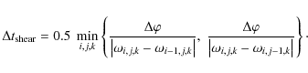(A.7)

The second restriction is only necessary in the case, where the above vertical averaging in Eq. (A.1) has not been performed. The sequencing of the advection sweeps in the FARGO algorithm has to be such that the azimuthal sweep comes at the end, hence in our simulations we use always: radial, meridional, and finally azimuthal.

In a staggered mesh code such as our NIRVANA code, that is essentially based on the ZEUS method, an additional complication arises in the straightforward application of the FARGO method, due to the fact that the velocity variables are located at the cell interfaces and not at the centres. Hence, the corresponding ``momentum cells'' for the radial and meridional momenta ( $\rho u_r$ and $\rho r u_\theta$ ) are shifted with respect to the standard density cells by half a gridcell in the radial or meridional direction, respectively. To apply the FARGO method one has first to split all the momentum cells in two halves, use the algorithm outlined above on each of the halves, and then combine them again afterwards to calculate from the updated momenta the new velocities on the interfaces. This leads of course to an overhead in the simulation cost which is counterbalanced however by the much larger time step.

Appendix B: Radiative transport

Here, we outline briefly the method to solve the flux-limited diffusion equation in 3D. Radiative transport is treated as a sub-step of the integration procedure. In equilibrium viscous heating is balancing radiative diffusion and to ensure this also numerically we incorporate the dissipation into this sub-step. Using the appropriate parts of the energy Eq. (7) and the flux (8) we obtain a diffusion equation for the gas temperature.

$\begin{displaymath}\frac{\partial T}{\partial t} = \frac{1}{c_{\rm v} \rho} ~ \left[ \nabla \cdot ~ D \nabla T + Q^+ \right] \end{displaymath}$

(B.1)

where the diffusion coefficient is given by

$\begin{displaymath}D = \frac{\lambda c 4 a_{\rm R} T^3}{\rho (\kappa + \sigma)}, \end{displaymath}$

(B.2)

and Q⁺ denotes the viscous dissipation that is added to the system. The flux-limiter $\lambda$ depends on the local physical state of the gas and approaches $\lambda = 1/3$ in the optically thick parts and reduces the flux to $F = c a_{\rm R} T^4$ in the optically thin parts. Here we use an expression for $\lambda$ as given in Kley (1989).

A straight forward finite difference form of Eq. (B.1) in Cartesian Coordinates is given by

	$\displaystyle \frac{T^{n+1}_{i,j,k} - T^n_{i,j,k}}{\Delta t}$ = $\displaystyle \frac{1}{(c{v} \rho)_{i,j,k}}$	(B.3)
	$\displaystyle \times \left[\frac{1}{\Delta x} \left( \bar{D}^x_{i+1,j,k} \frac{... ... x} - \bar{D}^x_{i,j,k} \frac{T_{i,j,k} - T_{i-1,j,k}}{\Delta x} \right)\right.$
	$\displaystyle + \frac{1}{\Delta y} \left( \bar{D}^y_{i,j+1,k} \frac{T_{i,j+1,k}... ...{\Delta y} - \bar{D}^y_{i,j,k} \frac{T_{i,j,k} - T_{i,j-1,k}}{\Delta y} \right)$
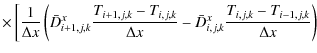
	$\displaystyle \left. + \frac{1}{\Delta z} \left( \bar{D}^z_{i,j,k+1} \frac{T_{i... ... \bar{D}^z_{i,j,k} \frac{T_{i,j,k} - T_{i,j,k-1}}{\Delta z} \right)\right]\cdot$

In orthogonal curvilinear coordinates additional geometry terms have to be added in the above equation. Here $\bar{D}^x_{i,j,k}$ denotes

$\begin{displaymath}\bar{D}^x_{i,j,k} = \frac{1}{2} \left( D_{i,j,k} + D_{i-1,j,k} \right) \end{displaymath}$

(B.4)

and so forth.

The grid structure from which Eq. (B.3) follows is outlined in the two-dimensional case in Fig. B.1. One has to keep in mind that the temperature (being a scalar) is defined in the cell centre, while the values of $\bar{D}^x_{i,j,k}$ are defined at the cell interfaces.

$\begin{figure} \par\includegraphics[width=8.5cm,clip]{12072fB1.eps} \end{figure}$

Figure B.1:

The grid structure used in a staggered grid code for a two-dimensional example. Shown is the cell i,j where the coordinates of the cell centre [ x^c_i, y^c_j] is given by [ 1/2(x_i,j+x_i+1,j), 1/2(y_i,j+y_i,j+1)]. The temperature T_i,j is located at the cell centre where also the diffusion coefficient D is defined. The averaged diffusion coefficients $\bar{D}$ are defined at the cell interfaces.

Open with DEXTER

In Eq. (B.3) no time levels are specified on the right hand side. For explicit differencing the time level should be tⁿ such that the new temperature on the left Tⁿ⁺¹ is entirely given by the old values Tⁿ at time tⁿ. This might lead to very small timesteps since the timestep limitation is approximately given by

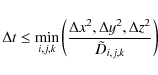$\begin{displaymath}\Delta t \leq \min_{i,j,k} \left( \frac{\Delta x^2, \Delta y^2, \Delta z^2}{ \tilde D_{i,j,k}} \right) \end{displaymath}$

(B.5)

where $\tilde D$ is given by $D/(\rho c_v)$ .

Hence, often an implicit version of the equation has to be used, where all the temperature values T_i,j,k on the r.h.s. are evaluated at the new time tⁿ⁺¹ or an arithmetic mean between new and old times. Even though the diffusion coefficients may depend on temperature, we always evaluate those at the old time tⁿ. Otherwise this would lead to a non-linear matrix equation.

Collection all the terms in Eq. (B.3) this leads to a linear system of equations with the form

A^x_i,j,k T_i-1,j,k + C^x_i,j,k T_i+1,j,k + A^y_i,j,k T_i,j-1,k + C^y_i,j,k T_i,j+1,k
A^z_i,j,k T_i,j,k-1 + C^z_i,j,k T_i,j,k+1 + B_i,j,k T_i,j,k = R_i,j,k			(B.6)

where the superscript n+1 has been omitted on the left hand side. The coefficients A^x_i,j,k to C^z_i,j,k can be obtained straightforwardly from Eq. (B.3). The right hand side is given by

$\begin{displaymath}R_{i,j,k} = T^{n}_{i,j,k} + \frac{1}{(c_v \rho)_{i,j,k}} ~ Q^{+}_{i,j,k} . \end{displaymath}$

Written in matrix notation Eq. (B.6) reads

$\begin{displaymath}{\sf M} \vec{T}^{n+1} = \vec{R}. \end{displaymath}$

(B.7)

Obviously the matrix ${\sf M}$ is a sparse matrix with a banded structure. Usually ${\sf M}$ is diagonally dominant but in situations with extended optically thin regions this property will be lost.

Equation (B.7) can in principle be solved by any linear equation package. For simplicity and testing purposes we work presently with a standard SOR solver. Using an optimised relaxation parameter $\tilde \omega$ we need about 130 iterations per timestep in the initial phase which is far from equilibrium and only 80 iterations at later times near equilibrium.

The radiation module of the code has been tested extensively in different coordinate systems in Bitsch (2008), and we have compared our new results on radiative viscous discs obtained with the 3D version of NIRVANA in detail with those of the existing 2D code RH2D.

References

Alibert, Y., Mordasini, C., & Benz, W. 2004, A&A, 417, L25 [NASA ADS] [CrossRef] [EDP Sciences]
Balbus, S. A., & Hawley, J. F. 1998, Rev. Mod. Phys., 70, 1 [NASA ADS] [CrossRef]
Baruteau, C., & Masset, F. 2008, ApJ, 672, 1054 [NASA ADS] [CrossRef]
Bitsch, B. 2008, Diploma Thesis, University of Tübingen
Cresswell, P., Dirksen, G., Kley, W., & Nelson, R. P. 2007, A&A, 473, 329 [NASA ADS] [CrossRef] [EDP Sciences]
Crida, A., Sándor, Z., & Kley, W. 2008, A&A, 483, 325 [NASA ADS] [CrossRef] [EDP Sciences]
D'Angelo, G., Henning, T., & Kley, W. 2002, A&A, 385, 647 [NASA ADS] [CrossRef] [EDP Sciences]
D'Angelo, G., Kley, W., & Henning, T. 2003, ApJ, 586, 540 [NASA ADS] [CrossRef]
Ida, S., & Lin, D. N. C. 2008, ApJ, 673, 487 [NASA ADS] [CrossRef]
Klahr, H., & Kley, W. 2006, A&A, 445, 747 [NASA ADS] [CrossRef] [EDP Sciences]
Kley, W. 1989, A&A, 208, 98 [NASA ADS]
Kley, W. 1998, A&A, 338, L37 [NASA ADS]
Kley, W., & Crida, A. 2008, A&A, 487, L9 [NASA ADS] [CrossRef] [EDP Sciences]
Kley, W., & Lin, D. N. C. 1996, ApJ, 461, 933 [NASA ADS] [CrossRef]
Kley, W., & Lin, D. N. C. 1999, ApJ, 518, 833 [NASA ADS] [CrossRef]
Kley, W., Papaloizou, J. C. B., & Lin, D. N. C. 1993, ApJ, 416, 679 [NASA ADS] [CrossRef]
Kley, W., D'Angelo, G., & Henning, T. 2001, ApJ, 547, 457 [NASA ADS] [CrossRef]
Levermore, C. D., & Pomraning, G. C. 1981, ApJ, 248, 321 [NASA ADS] [CrossRef]
Li, H., Lubow, S. H., Li, S., & Lin, D. N. C. 2009, ApJ, 690, L52 [NASA ADS] [CrossRef]
Lin, D. N. C., & Papaloizou, J. C. B. 1985, in Protostars and Planets II, 981
Masset, F. 2000a, A&AS, 141, 165 [NASA ADS] [CrossRef] [EDP Sciences]
Masset, F. S. 2000b, in Disks, Planetesimals, and Planets, ed. G. Garzón, C. Eiroa, D. de Winter, & T. J. Mahoney, ASP Conf. Ser., 219, 75
Masset, F. S. 2001, ApJ, 558, 453 [NASA ADS] [CrossRef]
Masset, F. S. 2002, A&A, 387, 605 [NASA ADS] [CrossRef] [EDP Sciences]
Masset, F. S. 2008, in EAS Publications Series, ed. M.-J. Goupil, & J.-P. Zahn, 29, 165
Masset, F. S., D'Angelo, G., & Kley, W. 2006, ApJ, 652, 730 [NASA ADS] [CrossRef]
Mihalas, D., & Weibel Mihalas, B. 1984, Foundations of radiation hydrodynamics (New York: Oxford University Press)
Ogilvie, G. I., & Lubow, S. H. 2003, ApJ, 587, 398 [NASA ADS] [CrossRef]
Paardekooper, S.-J., & Mellema, G. 2006, A&A, 459, L17 [NASA ADS] [CrossRef] [EDP Sciences]
Paardekooper, S.-J., & Mellema, G. 2008, A&A, 478, 245 [CrossRef] [EDP Sciences]
Paardekooper, S.-J., & Papaloizou, J. 2009, MNRAS, 394, 2283 [NASA ADS] [CrossRef]
Paardekooper, S.-J., & Papaloizou, J. C. B. 2008, A&A, 485, 877 [NASA ADS] [CrossRef] [EDP Sciences]
Papaloizou, J. C. B., Nelson, R. P., Kley, W., Masset, F. S., & Artymowicz, P. 2007, in Protostars and Planets V, ed. B. Reipurth, D. Jewitt, & K. Keil, 655
Stone, J. M., & Norman, M. L. 1992, ApJS, 80, 753 [NASA ADS] [CrossRef]
Tanaka, H., Takeuchi, T., & Ward, W. R. 2002, ApJ, 565, 1257 [NASA ADS] [CrossRef]
Tassoul, J. 1978, Theory of rotating stars, Princeton Series in Astrophysics (Princeton: University Press)
Ward, W. R. 1997, Icarus, 126, 261 [NASA ADS] [CrossRef]
Ziegler, U., & Yorke, H. 1997a, Computer Physics Commun., 101, 54 [NASA ADS] [CrossRef]
Ziegler, U., & Yorke, H. W. 1997b, Computer Physics Commun., 101, 54 [NASA ADS] [CrossRef]

All Figures

$\begin{figure} \par\includegraphics[width=9cm,clip]{12072fg01.eps} \end{figure}$	Figure 1: The gravitational potential of a $20~ M_{\rm earth}$ planet with different smoothings applied, see Eqs. (9) and (10). The distance d from the planet is given in units of $a_{\rm p}$ (here $a_{\rm Jup}$ ), and the smoothing length $r_{\rm sm}$ in units of the Hill radius of the planet which refers here to $R_{\rm H} = 0.0271 a_{\rm p}$ . Note that the data points are drawn directly from the used 3D computational grid and indicate our standard numerical resolution (see Sect. 2.4).
Open with DEXTER
In the text

$\begin{figure} \par\includegraphics[width=9cm,clip]{12072fg2a.eps}\par\includegr... ...{12072fg2b.eps}\par\includegraphics[width=9cm,clip]{12072fg2c.eps} \end{figure}$	Figure 2: Evolution of semi-major axis, eccentricity and inclination as a function of time for a 20 $M_{\rm earth}$ planet in a three-dimensional disc. Results are displayed for different numerical resolutions ( $N_r, N_\theta , N_\varphi$ ), and using Fargo and Non-Fargo runs.
Open with DEXTER
In the text

$\begin{figure} \par\includegraphics[width=4.4cm,clip]{12072fg3a.eps}\hspace*{1.5mm} \includegraphics[width=4.4cm,clip]{12072fg3b.eps} \end{figure}$	Figure 3: Radial stratification of surface density ( left) and the midplane temperature ( right) in the disc. This dashed lines represent simple approximations to the 3D stratified results. The solid (green) curves labelled ``flat'' refer to corresponding results for a vertically integrated flat 2D disc using the same input physics.
Open with DEXTER
In the text

$\begin{figure} \par\includegraphics[width=4.4cm,clip]{12072fg4a.eps}\hspace*{1.5mm} \includegraphics[width=4.4cm,clip]{12072fg4b.eps} \end{figure}$	Figure 4: Vertical stratification of density ( left) and temperature ( right) at a radius of r=1.44. Thin dashed lines just represent simple functional relations.
Open with DEXTER
In the text

$\begin{figure} \par\includegraphics[width=8cm,clip]{12072fg5a.eps} \includegraphics[width=8cm,clip]{12072fg5b.eps} \end{figure}$	Figure 5: Vertical stratification of density in logarithmic scale ( top) and temperature ( bottom) at a radius of r=1.00 for a simulation covering the $\theta = 90^\circ$ to $70^\circ$ region. The optical depth $\tau =1.0$ is reached at about z=0.055.
Open with DEXTER
In the text

$\begin{figure} \par\includegraphics[width=9cm,clip]{12072fg6a.eps}\\ [1mm] \includegraphics[width=9cm,clip]{12072fg6b.eps} \end{figure}$	Figure 6: Density ( top) and Temperature ( bottom) for a fully radiative model in a 2D axisymmetric simulation.
Open with DEXTER
In the text

$\begin{figure} \par\includegraphics[width=9cm,clip]{12072fg7.eps} \end{figure}$	Figure 7: Vertical density distribution at r=1.4 for a fully radiative model in a 2D axisymmetric simulation. ``+'': isothermal starting configuration, `` $\times$ '': relaxed radiation equilibrium configuration.
Open with DEXTER
In the text

$\begin{figure} \par\includegraphics[width=9cm,clip]{12072fg8a.eps}\par\includegraphics[width=9cm,clip]{12072fg8b.eps} \end{figure}$	Figure 8: Surface density distribution for isothermal simulations with H/r=0.05 at 100 planetary orbits. Displayed are results for the shallowest and deepest potential. Top: $\epsilon$ -potential with $r_{\rm sm}=0.8$ , bottom: cubic with $r_{\rm sm}=0.5$ .
Open with DEXTER
In the text

$\begin{figure} \par\includegraphics[width=9cm,clip]{12072fg9.eps} \end{figure}$	Figure 9: Radial density distribution in the equator along ( $\rho (r, \varphi =\pi , \theta =\pi /2)$ ), i.e. along a ray through the location of the planet for all 4 planetary potentials used.
Open with DEXTER
In the text

$\begin{figure} \par\includegraphics[width=9cm,clip]{12072f10a.eps}\\ [1mm] \includegraphics[width=9cm,clip]{12072f10b.eps} \end{figure}$	Figure 10: Specific torque (in units of $a_{\rm p}^2 \Omega _{\rm p}^2$ ) acting on the planet using 4 different smoothings for the planetary potential in the isothermal case with H/r = 0.05. Top: evolution of total torque with time. Bottom: radial variation of the specific torque density $\Gamma (r)$ at t=80 orbits.
Open with DEXTER
In the text

$\begin{figure} \par\includegraphics[width=9cm,clip]{12072f11a.eps}\\ [1mm] \includegraphics[width=9cm,clip]{12072f11b.eps} \end{figure}$	Figure 11: Specific torque acting on the planet using different grid resolutions for the isothermal case with H/r = 0.037. In all cases the cubic potential with $r_{\rm sm}=0.5$ has been used. Top: evolution of total torque with time. Bottom: radial variation of the specific torque density, at t=80 orbits for the standard and medium resolution, and at 60 orbits for the high resolution.
Open with DEXTER
In the text

$\begin{figure} \par\includegraphics[width=0.81\linwx]{12072f12a.eps}\vspace{0.5... ...vspace{0.58mm} \includegraphics[width=0.81\linwx]{12072f12d.eps} \end{figure}$	Figure 12: Surface density ( upper two panels) and temperature in the equatorial plane ( lower two) for fully radiative simulations at 100 planetary orbits. Displayed are results for the shallowest and deepest potential. Upper panels refer to the $\epsilon$ -potential with $r_{\rm sm}=0.8$ , and lower to the cubic-potential with $r_{\rm sm}=0.5$ , respectively.
Open with DEXTER
In the text

$\begin{figure} \par\includegraphics[width=9cm,clip]{12072f13a.eps} \includegraphics[width=9cm,clip]{12072f13b.eps} \end{figure}$	Figure 13: Radial density ( top) and temperature ( bottom) distribution in the equator along a ray through the location of the planet for all 4 planetary potentials used, for the fully radiative case.
Open with DEXTER
In the text

$\begin{figure} \par\includegraphics[width=9cm,clip]{12072f14a.eps} \includegraphics[width=9cm,clip]{12072f14b.eps} \end{figure}$	Figure 14: Specific torques acting on a 20 $M_{\rm earth}$ planet for different numerical potentials in the fully radiative case. Top: evolution of total torque with time. Bottom: radial variation of the specific torque for t=80 orbits.
Open with DEXTER
In the text

$\begin{figure} \par\includegraphics[width=9cm,clip]{12072f15a.eps}\\ \includegraphics[width=9cm,clip]{12072f15b.eps} \end{figure}$	Figure 15: Specific torque acting on the planet using different grid resolutions for the fully radiative case. In all cases the cubic potential with $r_{\rm sm}=0.5$ has been used. Top: evolution of total torque with time. Bottom: radial variation of the specific torque density at t=50 orbits.
Open with DEXTER
In the text

$\begin{figure} \par\includegraphics[width=9cm,clip]{12072f16.eps} \end{figure}$	Figure 16: Radial variation of the specific torque acting on the planet using different thermodynamical disc models. In all cases the cubic potential with $r_{\rm sm}=0.5$ and standard resolution have been used. The adiabatic model at t=10 corresponds to the time where the corresponding total torque has its maximum. The models at t=80 have all reached their equilibria.
Open with DEXTER
In the text

$\begin{figure} \par\includegraphics[width=9cm,clip]{12072f17a.eps} \includegraphics[width=9cm,clip]{12072f17b.eps} \end{figure}$	Figure 17: Results of a 2D fully radiative model using a resolution of $512 \times 1536$ gridcells. The gray dot indicates the location of the planet, and the curve its Roche lobe. The solid black lines show the streamlines. Top: perturbed surface density with respect to the case without an embedded planet. The values are scaled as $\Sigma ^{1/2}$ . Bottom: the net torque acting on the planet caused by the mass in each individual gridcell using the prescribed smoothed torque cutoff function with b=0.8, see explanation in text. The values are scaled as $(\tilde{\Gamma}^{\pm})^{1/2}$ .
Open with DEXTER
In the text

$\begin{figure} \par\includegraphics[width=9cm,clip]{12072f18a.eps} \includegraphics[width=9cm,clip]{12072f18b.eps} \end{figure}$	Figure 18: Perturbed entropy ( top) and perturbed density ( bottom) for the 2D fully radiative equilibrium model using a resolution of $512 \times 1536$ gridcells. The values are scaled as $\Sigma ^{1/2}$ and S^1/2, respectively.
Open with DEXTER
In the text

$\begin{figure} \par\includegraphics[width=9cm,clip]{12072f19.eps} \end{figure}$	Figure 19: Specific torques acting on planets of different masses in the fully radiative (blue crosses) and isothermal (red plus signs) regime. Note, that the isothermal models are run for a fixed H/r =0.037. All torque values are displayed at a time when the equilibrium has been reached.
Open with DEXTER
In the text

$\begin{figure} \par\includegraphics[width=9cm,clip]{12072f20.eps} \end{figure}$	Figure 20: Radial torque distribution in equilibrium for various planet masses. The vertical dotted line indicates the location of the maximum.
Open with DEXTER
In the text

$\begin{figure} \par\includegraphics[width=8.5cm,clip]{12072fB1.eps} \end{figure}$	Figure B.1: The grid structure used in a staggered grid code for a two-dimensional example. Shown is the cell i,j where the coordinates of the cell centre [ x^c_i, y^c_j] is given by [ 1/2(x_i,j+x_i+1,j), 1/2(y_i,j+y_i,j+1)]. The temperature T_i,j is located at the cell centre where also the diffusion coefficient D is defined. The averaged diffusion coefficients $\bar{D}$ are defined at the cell interfaces.
Open with DEXTER
In the text

Current usage metrics show cumulative count of Article Views (full-text article views including HTML views, PDF and ePub downloads, according to the available data) and Abstracts Views on Vision4Press platform.

Data correspond to usage on the plateform after 2015. The current usage metrics is available 48-96 hours after online publication and is updated daily on week days.

Initial download of the metrics may take a while.

Planet migration in three-dimensional radiative discs

1 Introduction

2 Physical modelling

2.1 Basic equations

2.2 Planetary potential

2.3 Setup

2.4 Numerics

3 Test calculations

3.1 The FARGO-algorithm

3.2 The radiation algorithm

3.3 Density floor

4 Models with an embedded planet

4.1 Initial setup

4.2 Isothermal discs

4.3 Fully radiative discs

4.4 Torque analysis for the radiative case

4.5 Planets with different planetary masses

5 Summary

Appendix A: Fargo algorithm

Appendix B: Radiative transport

References

All Figures

3.1 The `FARGO`-algorithm