| Issue |
A&A
Volume 506, Number 2, November I 2009
|
|
|---|---|---|
| Page(s) | 745 - 756 | |
| Section | Interstellar and circumstellar matter | |
| DOI | https://doi.org/10.1051/0004-6361/200811246 | |
| Published online | 18 August 2009 | |
A&A 506, 745-756 (2009)
Dust emissivity variations in the Milky
Way![[*]](/icons/foot_motif.png)
D. Paradis1,2,3 - J.-Ph. Bernard2,3 - C. Mény2,3
1 - Spitzer Science Center, California Institute of Technology,
Pasadena, CA 91125, USA
2 - Université de Toulouse, UPS, CESR, 9 Av. du Colonel Roche, 31028
Toulouse Cedex 9, France
3 - CNRS, UMR5187, 31028 Toulouse, France
Received 28 October 2008 / Accepted 3 July 2009
Abstract
Aims. Dust properties appear to vary according to
the environment in which the dust evolves. Previous observational
indications of these variations in the far-infrared (FIR) and
submillimeter (submm) spectral range are scarce and limited to specific
regions of the sky. To determine whether these results can be
generalised to larger scales, we study the evolution in dust
emissivities from the FIR to millimeter (mm) wavelengths, in the atomic
and molecular interstellar medium (ISM), along the Galactic plane
towards the outer Galaxy.
Methods. We correlate the dust FIR to mm emission
with the HI and CO emission, which are taken to trace
the atomic and molecular phases, respectively. The study is carried out
using the DIRBE data from 100 to 240
![]() ,
the Archeops data from 550
,
the Archeops data from 550
![]() to 2.1 mm, and the WMAP data at 3.2 mm (W band), in
regions with Galactic latitude
to 2.1 mm, and the WMAP data at 3.2 mm (W band), in
regions with Galactic latitude ![]() ,
over the Galactic longitude range (
,
over the Galactic longitude range (
![]() )
observed with Archeops. We estimate the average dust temperature in
each phase and divide the emission spectral energy distribution (SED)
by a black body at this temperature to derive the emissivity profile. A
detailed verification of the impact of the implied simplification, such
as temperature mixing along the line of sight, is provided.
)
observed with Archeops. We estimate the average dust temperature in
each phase and divide the emission spectral energy distribution (SED)
by a black body at this temperature to derive the emissivity profile. A
detailed verification of the impact of the implied simplification, such
as temperature mixing along the line of sight, is provided.
Results. In all regions studied, the emissivity
spectra in both the atomic and molecular phases are steeper in the FIR
(
![]() )
than in the submm and mm (
)
than in the submm and mm (![]() ). We find significant
variations in the spectral shape of the dust emissivity as a function
of the dust temperature in the molecular phase. Regions of similar dust
temperature in the molecular and atomic gas exhibit similar emissivity
spectra. Regions where the dust is significantly colder in the
molecular phase show a significant increase in emissivity for the range
100-550
). We find significant
variations in the spectral shape of the dust emissivity as a function
of the dust temperature in the molecular phase. Regions of similar dust
temperature in the molecular and atomic gas exhibit similar emissivity
spectra. Regions where the dust is significantly colder in the
molecular phase show a significant increase in emissivity for the range
100-550
![]() .
We exclude the possibility of this effect being an artifact of our
temperature determination or the assumptions made. This result supports
the hypothesis of grain coagulation in these regions, confirming
results obtained over small fractions of the sky in previous studies
and allowing us to expand these results to the cold molecular
environments in general of the outer MW. Possible reasons for
the observed emissivity increase in the molecular phase that vanishes
in the mm range are discussed by comparison with dust models, involving
dust aggregation and solid state physics processes specific to
amorphous material. We note that it is the first time that these
effects have been demonstrated by direct measurement of the emissivity,
while previous studies were based only on thermal arguments.
.
We exclude the possibility of this effect being an artifact of our
temperature determination or the assumptions made. This result supports
the hypothesis of grain coagulation in these regions, confirming
results obtained over small fractions of the sky in previous studies
and allowing us to expand these results to the cold molecular
environments in general of the outer MW. Possible reasons for
the observed emissivity increase in the molecular phase that vanishes
in the mm range are discussed by comparison with dust models, involving
dust aggregation and solid state physics processes specific to
amorphous material. We note that it is the first time that these
effects have been demonstrated by direct measurement of the emissivity,
while previous studies were based only on thermal arguments.
Key words: ISM: dust, extinction - infrared: ISM - submillimeter
1 Introduction
Measuring the dust emissivity is important to inferring the nature of
dust from its emission and also determining the dust heating
from its observed temperature. In addition, variations in the dust
emissivity may seriously affect the mass estimates inferred from
FIR to mm observations. Dust emissivity and its possible variations
with wavelength or temperature are also critical for separating
astrophysical foreground emission from the
cosmic microwave background (CMB). However, deriving dust
emissivity is generally a difficult task because it relies on both
estimating the dust temperature and the gas column density associated
with the emitting dust. Big dust Grains (BG, see Désert
et al. 1990, for a
description of each dust component) are in thermal
equilibrium with the interstellar radiation field (ISRF). Their
emission is close to that of a gray-body with an equilibrium
temperature near
17.5 K in the diffuse ISM (Boulanger et al. 1996;
Lagache
et al. 1998), with a
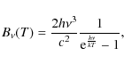
maximum in the far-infrared. The emission spectrum, assuming a fixed
dust abundance and a single grain size, follows
where
Although, in principle, the emissivity may depend on
wavelength and
temperature (e.g., Mény et al.
2007), it has been customary to assume no
temperature dependence and a power law distribution with frequency,
where
A decrease in the IRAS ![]() ratio in several
isolated molecular clouds has also been noted
(e.g., Laureijs
et al. 1991; Abergel et al. 1995,1994),
whereas this ratio
seems to be constant in diffuse regions. This could be interpreted as
a decrease of very small grain (VSG) abundance with respect to
that
of the BGs in dense molecular clouds. Bernard
et al. (1999) analysed the
FIR dust emission from a molecular cirrus in Polaris, using the PRONAOS
balloon-borne experiment data and found a larger decrease in the
BG equilibrium temperature than predicted from the decrease in
the ISRF
intensity in the cloud. The same region showed an obvious deficit in
60
ratio in several
isolated molecular clouds has also been noted
(e.g., Laureijs
et al. 1991; Abergel et al. 1995,1994),
whereas this ratio
seems to be constant in diffuse regions. This could be interpreted as
a decrease of very small grain (VSG) abundance with respect to
that
of the BGs in dense molecular clouds. Bernard
et al. (1999) analysed the
FIR dust emission from a molecular cirrus in Polaris, using the PRONAOS
balloon-borne experiment data and found a larger decrease in the
BG equilibrium temperature than predicted from the decrease in
the ISRF
intensity in the cloud. The same region showed an obvious deficit in
60
![]() emission. They
attributed the change in the particular dust
properties of dense environments.
emission. They
attributed the change in the particular dust
properties of dense environments.
Stepnik et al.
(2003) attempted to explain the origin of the decrease in
VSG abundance and the drop in the BG temperature in dense
environments. They measured a BG temperature of
16.8 K outside a
filament in Taurus, and of 12 K at the centre of the filament,
using
the PRONAOS and the IRAS data. They showed that a model that assumed
the standard
properties of dust, without any spatial variations in the grain
properties, was unable to reproduce the observations. The
attenuation of the radiation field in the cloud was also unable to
explain the
shape of the observed emission profiles. They proposed that the
aggregation of large dust grains and most of the VSGs in fractal
assemblies would explain both the observed 60
![]() emission
deficit and the unusually cold BG temperature. They showed that
aggregation would lead to an increase in the BG emissivities by a
factor of 3-4, and that between 80 and 100
emission
deficit and the unusually cold BG temperature. They showed that
aggregation would lead to an increase in the BG emissivities by a
factor of 3-4, and that between 80 and 100![]() of the VSGs should participate in
the aggregation process. The best-fit model showed that the VSG and BG
aggregation occurs at an extinction
of the VSGs should participate in
the aggregation process. The best-fit model showed that the VSG and BG
aggregation occurs at an extinction ![]() mag
and at
densities higher than
mag
and at
densities higher than ![]() H/cm3.
However, the emissivity
increase in dense environments remains indirect evidence of change in
the emissivity, since
H/cm3.
However, the emissivity
increase in dense environments remains indirect evidence of change in
the emissivity, since
![]() is lower
than expected for the corresponding ISRF. This
effect has never been illustrated by a direct
determination of the dust emissivity, mainly because both the dust
temperature and
is lower
than expected for the corresponding ISRF. This
effect has never been illustrated by a direct
determination of the dust emissivity, mainly because both the dust
temperature and ![]() are difficult to measure.
are difficult to measure.
Cambrésy et al.
(2001a) analysed the DIRBE emission of the Polaris complex
over 20 deg2, to determine the dust
properties. They decomposed the emission into a warm and a cold
component constrained using the ![]() IRAS
intensity ratio. They determined the extinction map of this complex in
the visible, by using star counts in the V band
(Cambrésy 1999). They
calculated the submillimeter emissivity of
each component, normalised to the visible extinction, and found
that the emissivity is 4 times higher in the cold region of
the complex than in the warm region. This result matches the emissivity
increase
derived to explain the low dust temperature by Stepnik
et al. (2003), and was based on the determination of
the submm to
visible dust opacity ratio, which traces the optical properties
of the grain material, independent of the gas column density.
IRAS
intensity ratio. They determined the extinction map of this complex in
the visible, by using star counts in the V band
(Cambrésy 1999). They
calculated the submillimeter emissivity of
each component, normalised to the visible extinction, and found
that the emissivity is 4 times higher in the cold region of
the complex than in the warm region. This result matches the emissivity
increase
derived to explain the low dust temperature by Stepnik
et al. (2003), and was based on the determination of
the submm to
visible dust opacity ratio, which traces the optical properties
of the grain material, independent of the gas column density.
Two hypotheses have been proposed to explain the observations:
the
formation of ice mantles (Laureijs et al. 1991,1996)
and/or grain
aggregation (Draine
& Anderson 1985; Tielens 1989). The 60
![]() emission
deficit in dense regions can be attributed to a large
majority of VSGs participating in the aggregation process, and the VSGs
are almost totally accreted onto the aggregates, in the inner regions
of
the cloud (Stepnik et al.
2003). The VSGs are then connected to the
aggregate, which acts as a thermostat. Their temperature then stops
fluctuating and their contribution to the mid-IR greatly decreases,
which
explains their weak IRAS 60
emission
deficit in dense regions can be attributed to a large
majority of VSGs participating in the aggregation process, and the VSGs
are almost totally accreted onto the aggregates, in the inner regions
of
the cloud (Stepnik et al.
2003). The VSGs are then connected to the
aggregate, which acts as a thermostat. Their temperature then stops
fluctuating and their contribution to the mid-IR greatly decreases,
which
explains their weak IRAS 60
![]() emission. Calculations, for
instance using the discrete dipole approximation (DDA) method, of
optical properties of aggregates (Bazell
& Dwek 1990) show that BG aggregates are
more efficient emitters than a collection of individual grains. This
increased emissivity leads to more efficient
cooling for a given ISRF intensity and therefore explains the lower
temperature observed. The calculations indicate that the aggregate
emissivity should progressively deviate from that of the individual
grains in the IR (around 20
emission. Calculations, for
instance using the discrete dipole approximation (DDA) method, of
optical properties of aggregates (Bazell
& Dwek 1990) show that BG aggregates are
more efficient emitters than a collection of individual grains. This
increased emissivity leads to more efficient
cooling for a given ISRF intensity and therefore explains the lower
temperature observed. The calculations indicate that the aggregate
emissivity should progressively deviate from that of the individual
grains in the IR (around 20
![]() ), and remain parallel to it
at
longer wavelengths, in particular over the entire submillimeter and
millimeter range.
), and remain parallel to it
at
longer wavelengths, in particular over the entire submillimeter and
millimeter range.
The adjunction of VSGs in the aggregate seems to have little effect on FIR/mm properties and simply provides a slightly higher absorptivity of the aggregate in the near-IR (Stepnik 2001a). Calculations by Stepnik et al. (2003) show that a total number of at least 20 individual BG in each aggregate is necessary to provide the required emissivity increase. However, for the aggregation process to be efficient, the individual grains should probably be covered with an ice mantle, to increase the sticking efficiency.
The parameter ![]() in Eq. (1)
is consistent with the
definition used in Boulanger
et al. (1996). The emissivity
in Eq. (1)
is consistent with the
definition used in Boulanger
et al. (1996). The emissivity ![]() is related
to the absorption efficiency
is related
to the absorption efficiency ![]() ,
which is directly
related to the refractive index of the material composing the grain by
,
which is directly
related to the refractive index of the material composing the grain by
where a is the grain radius. Therefore, for a single grain size, the wavelength dependence of
In Sect. 2, we present the data that we used for our study and in Sect. 3 we define the emission to column density conversion factors used. In Sect. 4, we describe the correlation procedure between dust emission and gas tracers. In Sect. 5, we explain how we compute the grain emissivity. The results of this study and the verification of our hypothesis of a single temperature along the LOS are presented in Sects. 6 and 7. Sections 8 and 9 are devoted to our discussion and conclusions.
2 Data
2.1 FIR data
The Diffuse Infrared Background Experiment (DIRBE) was an infrared
photometer onboard the COBE satellite (launched in 1989) to
measure the diffuse infrared and microwave radiation from the early
universe. It observed the entire sky at 10 different
wavelengths between 1 and
240
![]() ,
with a 40
,
with a 40
![]() instantaneous angular
resolution. However, the asymmetric beam of the DIRBE instrument
convolved with the spinning of the instrument produced an effective
beam of
instantaneous angular
resolution. However, the asymmetric beam of the DIRBE instrument
convolved with the spinning of the instrument produced an effective
beam of ![]()
![]() in the yearly averaged products
(Cambrésy et al. 2001b).
For our study, we only consider data in the far-infrared
at 100, 140, and 240
in the yearly averaged products
(Cambrésy et al. 2001b).
For our study, we only consider data in the far-infrared
at 100, 140, and 240
![]() ,
since emission at shorter
wavelengths contains a large contribution from thermally
fluctuating VSGs and polycyclic aromatic hydrocarbons (PAH). The DIRBE
data at these wavelengths were calibrated with models for Uranus
(100
,
since emission at shorter
wavelengths contains a large contribution from thermally
fluctuating VSGs and polycyclic aromatic hydrocarbons (PAH). The DIRBE
data at these wavelengths were calibrated with models for Uranus
(100
![]() )
and Jupiter (140 and 240
)
and Jupiter (140 and 240
![]() )
together with in-flight
beam shape measurements. This calibration matched that of the
FIRAS instrument, which incorporated an absolute
calibrator, within a small correction factor, which we did not
apply in this study since it is smaller than our uncertainties (Fixen et al. 1997).
)
together with in-flight
beam shape measurements. This calibration matched that of the
FIRAS instrument, which incorporated an absolute
calibrator, within a small correction factor, which we did not
apply in this study since it is smaller than our uncertainties (Fixen et al. 1997).
Archeops was a balloon-borne experiment dedicated to
the measure of
the temperature fluctuations in the CMB. The focal plane instrument, a
multi-band photometer, worked in four bands centered on 550
![]() ,
850
,
850
![]() ,
1.4 mm, and 2.1 mm. Archeops had an angular
resolution of 8
,
1.4 mm, and 2.1 mm. Archeops had an angular
resolution of 8
![]() (see Benoit et al. 2002,
for a full
description of the instrument). We use data obtained during
the last flight of the instrument from Kiruna in
February 2002, which
covered about 30
(see Benoit et al. 2002,
for a full
description of the instrument). We use data obtained during
the last flight of the instrument from Kiruna in
February 2002, which
covered about 30![]() of the sky. We note that we limit our analysis
to the region surveyed by Archeops, which is given by the range of
Galactic
longitudes
of the sky. We note that we limit our analysis
to the region surveyed by Archeops, which is given by the range of
Galactic
longitudes ![]() ,
in the second and third Galactic quadrants. The Archeops data were
calibrated against the FIRAS maps, at 550
,
in the second and third Galactic quadrants. The Archeops data were
calibrated against the FIRAS maps, at 550
![]() and 850
and 850
![]() ,
and with respect to the CMB dipole at 1.4 mm and
2.1 mm. We note that the calibration of the Archeops data
should be accurate at
all wavelengths, since it relies on the FIRAS maps at high
frequencies, which are absolutely calibrated to
,
and with respect to the CMB dipole at 1.4 mm and
2.1 mm. We note that the calibration of the Archeops data
should be accurate at
all wavelengths, since it relies on the FIRAS maps at high
frequencies, which are absolutely calibrated to ![]() (Fixsen et al. 1994),
and on the CMB dipole at low frequencies, whose brightness is
accurately known. In addition, the Archeops cosmology results derived
from the low frequency channels have been shown to be consistent with
those of the WMAP satellite at the
(Fixsen et al. 1994),
and on the CMB dipole at low frequencies, whose brightness is
accurately known. In addition, the Archeops cosmology results derived
from the low frequency channels have been shown to be consistent with
those of the WMAP satellite at the ![]() accuracy (Tristram et al.
2005).
Details of the Archeops data processing are given in
Macias-Perez et al. (2007).
We note that the Archeops channel at 550
accuracy (Tristram et al.
2005).
Details of the Archeops data processing are given in
Macias-Perez et al. (2007).
We note that the Archeops channel at 550
![]() has residual stripes, because
only one detector was
available at that frequency.
has residual stripes, because
only one detector was
available at that frequency.
The Wilkinson Microwave Anisotropy Probe (WMAP) measured the
emission
over the entire sky in the microwave range (3.2-13 mm), and
provided
accurate maps of the CMB fluctuations. The WMAP data, with
a 13
![]() beam, is currently the instrument of the highest angular resolution
covering the entire sky in this wavelength domain. Here, we use only
the W band data (3.2 mm), because the other bands are often
dominated by gas emission, such as free-free and synchrotron, or
by the anomalous foreground emission
(see Draine
& Lazarian 1998; Bennett et al. 2003),
presumably because of small spinning
particles. The calibration of the WMAP data was completed using the CMB
dipole amplitude (see Hinshaw
et al. 2003).
beam, is currently the instrument of the highest angular resolution
covering the entire sky in this wavelength domain. Here, we use only
the W band data (3.2 mm), because the other bands are often
dominated by gas emission, such as free-free and synchrotron, or
by the anomalous foreground emission
(see Draine
& Lazarian 1998; Bennett et al. 2003),
presumably because of small spinning
particles. The calibration of the WMAP data was completed using the CMB
dipole amplitude (see Hinshaw
et al. 2003).
2.2 Gas tracers
We use the Leiden/Dwingeloo survey by Hartmann
& Burton (1996) for the HI data, with
sky observations above -30
![]() of Galactic latitude, obtained
with the 25 m Dwingeloo telescope, whose angular resolution
is 36
of Galactic latitude, obtained
with the 25 m Dwingeloo telescope, whose angular resolution
is 36
![]() (see Hartmann 1994, for
more details).
(see Hartmann 1994, for
more details).
We use ![]() data compiled by Dame et al.
(2001). These observations were obtained
along the Galactic plane in a Galactic latitude range from 4
data compiled by Dame et al.
(2001). These observations were obtained
along the Galactic plane in a Galactic latitude range from 4
![]() to 10
to 10
![]() ,
with an angular resolution of 7.5
,
with an angular resolution of 7.5
![]() ,
and some observations of large clouds at higher latitude,
with an angular resolution of 15
,
and some observations of large clouds at higher latitude,
with an angular resolution of 15
![]() .
The spatial coverage
is about 45
.
The spatial coverage
is about 45![]() of the sky.
of the sky.
All data were projected onto the HEALPix pixelisation scheme
(Hierarchical Equal Area isoLatitude Pixelisation)![]() with a nside = 128, corresponding to
a pixel size of 0.45
with a nside = 128, corresponding to
a pixel size of 0.45
![]() .
For the Archeops and WMAP first
release data, we use the published maps, and for HI and CO, we use the
maps
available on the WMAP lambda web site
.
For the Archeops and WMAP first
release data, we use the published maps, and for HI and CO, we use the
maps
available on the WMAP lambda web site![]() .
For the DIRBE data, we used our own
resampling method developed in the context of the ancillary data
for the Planck mission, computing the pixel intersection between the
original DIRBE maps in the sixcube format and the HEALPix
pixelisation. The method
preserves the photometry without significantly affecting the angular
resolution. Since the Archeops data were filtered to subtract
slow drifts, we simulated fake data stream with all data described in
this section, according to the actual Archeops scanning
strategy. Those data time-lines were treated in a similar way to the
Archeops
ones, in particular by including the low frequency filtering applied to
the Archeops data, and were then reprojected into sky maps. Using the
standard HEALPix tools, all the data were corrected to the DIRBE
angular resolution (1
.
For the DIRBE data, we used our own
resampling method developed in the context of the ancillary data
for the Planck mission, computing the pixel intersection between the
original DIRBE maps in the sixcube format and the HEALPix
pixelisation. The method
preserves the photometry without significantly affecting the angular
resolution. Since the Archeops data were filtered to subtract
slow drifts, we simulated fake data stream with all data described in
this section, according to the actual Archeops scanning
strategy. Those data time-lines were treated in a similar way to the
Archeops
ones, in particular by including the low frequency filtering applied to
the Archeops data, and were then reprojected into sky maps. Using the
standard HEALPix tools, all the data were corrected to the DIRBE
angular resolution (1
![]() ), by convolution with a
Gaussian
kernel of an appropriate size in relation to the original resolution of
each
dataset.
), by convolution with a
Gaussian
kernel of an appropriate size in relation to the original resolution of
each
dataset.
3 Conversion factors
Assuming that the gas is optically thin, the hydrogen column density can be deduced from the integrated intensity of the HI emission at 21 cm (| (4) |
where
 |
(5) |
This value was inferred from
4 Correlation between IR and gas tracers
We considered only regions along the Galactic plane with ![]() and pixels with sufficient HI or CO emission
(
and pixels with sufficient HI or CO emission
(
![]() and
and ![]() ).
To assess the possible
contribution from free-free,
synchrotron, and spinning dust emission on the IR emission in the WMAP
W
band, we used the Planck Sky Model
).
To assess the possible
contribution from free-free,
synchrotron, and spinning dust emission on the IR emission in the WMAP
W
band, we used the Planck Sky Model![]() (Delabrouille et al.
2009).
The model indicates that the free-free emission is the main
contribution in this band and generates about 30
(Delabrouille et al.
2009).
The model indicates that the free-free emission is the main
contribution in this band and generates about 30![]() of the IR emission. Its contribution was subtracted from the W
band
emission, using the free-free map predicted by the Planck Sky Model.
Other
contaminations (synchrotron, spinning dust) are negligible
in this band (<3
of the IR emission. Its contribution was subtracted from the W
band
emission, using the free-free map predicted by the Planck Sky Model.
Other
contaminations (synchrotron, spinning dust) are negligible
in this band (<3![]() ),
according to the same
model. The contributions from free-free, synchrotron, and spinning dust
are insignificant in other data used in this study.
),
according to the same
model. The contributions from free-free, synchrotron, and spinning dust
are insignificant in other data used in this study.
We performed correlations between the infrared emission and
gas
tracers, in a set of rectangular regions covering the area of
interest. Individual regions have sizes ![]() ,
distributed across a regular grid
of Galactic coordinates every 3
,
distributed across a regular grid
of Galactic coordinates every 3
![]() in longitude and 2
in longitude and 2
![]() in latitude. In each region and each map, we subtracted a
background value computed as the median over a common background area,
defined to be the faintest half of the HI data. In this way,
we ensured
that the correlation produces a null IR emission for a null column
density. This step also removes any possible residual contribution
from both the Zodiacal light and the cosmic infrared background. We
then determined the best-fit linear correlation between the
FIR emission and gas tracers using
in latitude. In each region and each map, we subtracted a
background value computed as the median over a common background area,
defined to be the faintest half of the HI data. In this way,
we ensured
that the correlation produces a null IR emission for a null column
density. This step also removes any possible residual contribution
from both the Zodiacal light and the cosmic infrared background. We
then determined the best-fit linear correlation between the
FIR emission and gas tracers using
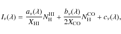
where
In a second step, we rejected regions of smaller than 15
pixels to maintain a sufficient number of pixels to perform the
correlations. The number of pixels in each region is given in tables in
the Appendix. With this selection, we removed 15![]() of the regions. In
a third step, we removed regions with clearly unphysical values of the
dust temperatures (>1000 K). For temperatures inferred
from
the spectral shape of
of the regions. In
a third step, we removed regions with clearly unphysical values of the
dust temperatures (>1000 K). For temperatures inferred
from
the spectral shape of ![]() and
and ![]() between 100 and
550
between 100 and
550
![]() (see Sect. 5
for more explanation),
these unphysical values imply that at least one of the correlation
coefficients
(see Sect. 5
for more explanation),
these unphysical values imply that at least one of the correlation
coefficients ![]() or
or ![]() in this wavelength range
is still affected by uncorrected instrumental effects, mostly residual
stripes in the Archeops 550
in this wavelength range
is still affected by uncorrected instrumental effects, mostly residual
stripes in the Archeops 550
![]() channel. This selection
removed 27
channel. This selection
removed 27![]() of the remaining regions.
of the remaining regions.
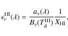
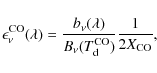
5 Grain emissivity determination
5.1 Method
Using Eqs. (1)
and (6),
and assuming a single
temperature of dust in the atomic (
![]() )
and the molecular
(
)
and the molecular
(
![]() )
phases, the emissivity of the dust associated with each
phase can be written
)
phases, the emissivity of the dust associated with each
phase can be written
and
respectively. The values of the dust temperatures in the two phases can be obtained by fitting the SED of the correlation coefficients
 |
(9) |
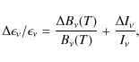
where the uncertainties on the intensity for the atomic and molecular phase are given by
 |
(10) |
the relative error in
 |
(11) |
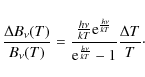
Errors in temperature used to derive the error in the Planck function are determined using a bootstrap method, when fitting for the temperature and spectral index. We note that the temperatures are mostly constrained by values close to the peak of the emission (i.e., 100, 140, and 240
All data used in this study follow a given flux convention
(e.g., ![]() for DIRBE data), which allows us to compute unambiguously the total
power received in the instrument
photometric band, regardless of the energy distribution in the
band. However, the true brightness at the reference frequency depends
on the emission spectral shape, which is unknown until a fit using a
model has
converged. We therefore corrected the emissivity derived above by
dividing by the appropriate color correction factor, computed using
the filter transmission and flux convention of each instrument
used. This was done in an iterative way, starting from color
correction factors derived from a dust model, and iterating for the
true shape of each SED, until convergence was reached.
for DIRBE data), which allows us to compute unambiguously the total
power received in the instrument
photometric band, regardless of the energy distribution in the
band. However, the true brightness at the reference frequency depends
on the emission spectral shape, which is unknown until a fit using a
model has
converged. We therefore corrected the emissivity derived above by
dividing by the appropriate color correction factor, computed using
the filter transmission and flux convention of each instrument
used. This was done in an iterative way, starting from color
correction factors derived from a dust model, and iterating for the
true shape of each SED, until convergence was reached.
5.2 Classification according to dust temperature
Dust in dense molecular clouds is expected to be colder than in the
surrounding atomic material, as long as no significant star formation
is occurring in the cloud. However, massive star formation can
significantly heat the dust in molecular clouds. In addition, star
formation may increase significantly the turbulence in the star-forming
molecular medium, which in turn, could modify the dust emission
properties. To search for these potential variations, we
classify the regions according to 3 categories based upon the
dust
temperature derived for dust in the atomic phase (
![]() )
and in the molecular phase (
)
and in the molecular phase (
![]() ):
):
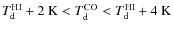
- regular: atomic and molecular medium with similar dust
temperatures defined as
 .
This
case allows us to compare the dust emissivity in the two environments
in
regions where the ISRF intensity is similar in both phases. This
category accounts for 18 regions in our sample;
.
This
case allows us to compare the dust emissivity in the two environments
in
regions where the ISRF intensity is similar in both phases. This
category accounts for 18 regions in our sample;
- colder CO: dust in the molecular phase significantly colder
than in the
atomic phase:
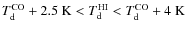 .
In this
case, the colder dust temperature in the molecular phase is indicative
of a
lower ISRF intensity in the cloud, most likely indicating dense
molecular environment with little star formation. This case is the
most relevant to the search for emissivity variations linked to the
formation of dust aggregates, since so far, these have been found
in such regions (see e.g., Stepnik et al. 2003; Bernard
et al. 1999). This category
accounts for 45 regions in our sample;
.
In this
case, the colder dust temperature in the molecular phase is indicative
of a
lower ISRF intensity in the cloud, most likely indicating dense
molecular environment with little star formation. This case is the
most relevant to the search for emissivity variations linked to the
formation of dust aggregates, since so far, these have been found
in such regions (see e.g., Stepnik et al. 2003; Bernard
et al. 1999). This category
accounts for 45 regions in our sample;
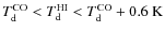
- warmer CO: dust in the atomic phase significantly colder
than in the
molecular phase:
 .
This
category should incorporate most of the massive star-forming regions.
The lower temperature (here
.
This
category should incorporate most of the massive star-forming regions.
The lower temperature (here  )
is lower than in the
previous case 2 in order to include enough regions. This
category
accounts for 25 regions in our sample.
)
is lower than in the
previous case 2 in order to include enough regions. This
category
accounts for 25 regions in our sample.
6 Results
![\begin{figure}
\par\includegraphics[width=8.7cm]{fig/11246fg1.eps}
\end{figure}](/articles/aa/full_html/2009/41/aa11246-08/img107.png) |
Figure 1: Studied regions for each temperature case: case 1 (regular) in white, case 2 (colder CO) in grey and case 3 (warmer CO) in black. The sky region covered by the Archeops data is also delineated. The coordinate grid shown is in Galactic coordinates. The map shows half the sky and is centered roughly towards the Galactic anticenter. |
| Open with DEXTER | |
![\begin{figure}
\par\includegraphics[width=8.7cm]{fig/11246fg2.eps}
\end{figure}](/articles/aa/full_html/2009/41/aa11246-08/img108.png) |
Figure 2: Dust temperature histograms for each selected case: the atomic and molecular phases are shown in dark grey with black contours and light grey, respectively. |
| Open with DEXTER | |
![\begin{figure}
\par\includegraphics[width=8cm]{fig/11246fg3.eps}
\end{figure}](/articles/aa/full_html/2009/41/aa11246-08/img110.png) |
Figure 3:
Median dust emissivity SEDs for case 1 (regular: upper panel),
case
2 (colder CO: middle panel) and case 3
(warmer CO: lower panel). The
DIRBE, Archeops and WMAP data correspond to diamond, star, and
square
symbols, respectively. The shaded areas show the |
| Open with DEXTER | |
Figure 3 shows the SEDs of the median emissivity derived from the correlation values, for the atomic and molecular phases, for each of the cases described in Sect. 5.2. The corresponding values are also given in Table 1.
The emissivity values shown in Fig. 3 were not
normalised in any other way than assuming the fixed conversion factors
described in Sect. 3.
In Fig. 3,
we also show the emissivity value derived from the FIRAS
data by Boulanger et al.
(1996) for the atomic diffuse ISM in the solar
neighbourhood at ![]() ,
assuming
,
assuming ![]() .
It can be seen
that the emissivity values derived here are in rough agreement with
that value. We note however that the atomic emissivities that we
derived
are somewhat higher than in the solar neighbourhood. We also note that
there is a continuity in the emissivity SED between
the WMAP W band and the Archeops range indicating that there
is no
obvious calibration difference between the two experiments, which are
both calibrated to the CMB dipole in this range.
.
It can be seen
that the emissivity values derived here are in rough agreement with
that value. We note however that the atomic emissivities that we
derived
are somewhat higher than in the solar neighbourhood. We also note that
there is a continuity in the emissivity SED between
the WMAP W band and the Archeops range indicating that there
is no
obvious calibration difference between the two experiments, which are
both calibrated to the CMB dipole in this range.
The scaling of emissivity values for the molecular phase can
be
modified by assuming a different ![]() factor. The
factor. The ![]() factor is difficult to determine. It is expected
to vary with various factors such as the metallicity and the chemistry
of the ISM, and could therefore change from cloud to
cloud (e.g., Magnani &
Onello 1995). In Fig. 4,
we show the same emissivity SEDs, where we have arbitrarily chosen the
factor is difficult to determine. It is expected
to vary with various factors such as the metallicity and the chemistry
of the ISM, and could therefore change from cloud to
cloud (e.g., Magnani &
Onello 1995). In Fig. 4,
we show the same emissivity SEDs, where we have arbitrarily chosen the
![]() value so that the atomic and molecular emissivities match at
the longest wavelengths. For each case, the derived
value so that the atomic and molecular emissivities match at
the longest wavelengths. For each case, the derived ![]() values are
given in the plot. Figure 4 more
clearly shows
the variations in the spectral shape. From that figure it is apparent
that in case 1 and 3, the atomic and molecular medium
emissivity SEDs
are almost parallel, while in case 2 (colder CO), the
molecular
emissivity SED is significantly steeper than the atomic one in the
FIR range. We note however, that if the absolute
level of the emissivities in the molecular phase can vary according to
the assumed
values are
given in the plot. Figure 4 more
clearly shows
the variations in the spectral shape. From that figure it is apparent
that in case 1 and 3, the atomic and molecular medium
emissivity SEDs
are almost parallel, while in case 2 (colder CO), the
molecular
emissivity SED is significantly steeper than the atomic one in the
FIR range. We note however, that if the absolute
level of the emissivities in the molecular phase can vary according to
the assumed ![]() value,
the spectral shape of the emissivity SED and therefore the emissivity
slope (
value,
the spectral shape of the emissivity SED and therefore the emissivity
slope (![]() )
will remain unchanged.
)
will remain unchanged.
In Fig. 4,
we also show power laws with
![]() ,
,
![]() and
and ![]() normalised at 100
normalised at 100
![]() for the atomic
phase. Although all emissivity SEDs globally show the expected
decrease with wavelength, it can be seen that,
in all 3 cases, the emissivity SED is steeper in the FIR (DIRBE data)
and flattens significantly in the submillimeter above
for the atomic
phase. Although all emissivity SEDs globally show the expected
decrease with wavelength, it can be seen that,
in all 3 cases, the emissivity SED is steeper in the FIR (DIRBE data)
and flattens significantly in the submillimeter above ![]() (Archeops and WMAP data). Tables 2 and 3
summarise the median values of the emissivity
spectral index at all wavelengths in the DIRBE and
Archeops wavelength ranges, respectively. These values were
inferred from a
linear adjustment of the emissivity SEDs. Uncertainties correspond to
1-
(Archeops and WMAP data). Tables 2 and 3
summarise the median values of the emissivity
spectral index at all wavelengths in the DIRBE and
Archeops wavelength ranges, respectively. These values were
inferred from a
linear adjustment of the emissivity SEDs. Uncertainties correspond to
1-![]() .
It can be seen that the emissivity index is generally
higher than
.
It can be seen that the emissivity index is generally
higher than ![]() in the FIR corresponding to a steep
emissivity decrease with wavelength, and is about
in the FIR corresponding to a steep
emissivity decrease with wavelength, and is about ![]() in
the submm and mm domain, corresponding to a flatter
spectrum. Apart from this common behavior, there are also significant
differences between the 3 temperature cases, which are
discussed
below.
in
the submm and mm domain, corresponding to a flatter
spectrum. Apart from this common behavior, there are also significant
differences between the 3 temperature cases, which are
discussed
below.
6.1 Case 1: regular
In this case, the emissivity SED of the dust associated with the atomic and molecular phases are almost parallel, and both clearly experience the same slope change between the DIRBE and the Archeops wavelengths. This similarity probably indicates that, in this case, the dust emission properties associated with the molecular and atomic phases are the same.
In addition, the absolute emissivity values in the two phases
are
relatively close. This indicates that our adopted ![]() value is
reasonable in that case. There is no reason in principle that the
dust abundance
value is
reasonable in that case. There is no reason in principle that the
dust abundance ![]() could differ between the two
phases. Therefore, an incorrect estimate of the
could differ between the two
phases. Therefore, an incorrect estimate of the ![]() parameter would produce
a wavelength-independent difference between the two emissivity
SEDs. Looking at the median values of
the emissivity ratios in the two phases presented in
Table 4,
we can see that the emissivity in the
atomic phase is higher that in the molecular phases at all
wavelengths, by about 30
parameter would produce
a wavelength-independent difference between the two emissivity
SEDs. Looking at the median values of
the emissivity ratios in the two phases presented in
Table 4,
we can see that the emissivity in the
atomic phase is higher that in the molecular phases at all
wavelengths, by about 30![]() for the assumed
for the assumed ![]() .
This difference
could be accounted for by a change in the
.
This difference
could be accounted for by a change in the ![]() value, which would
then have to be slightly lower than the one assumed,
value, which would
then have to be slightly lower than the one assumed, ![]() .
.
Table 1: Median values of the dust emissivity in the molecular and the atomic phase for each studied case: case 1 (regular), case 2 (colder CO), case 3 (warmer CO).
Table 2:
Median values of the emissivity spectral index (![]() )
in the
molecular and the atomic phase for each studied case and each
wavelength.
)
in the
molecular and the atomic phase for each studied case and each
wavelength.
Table 3:
Median values of the emissivity spectral index (![]() )
for the
FIR and submm domain, for each studied cases.
)
for the
FIR and submm domain, for each studied cases.
6.2 Case 2: colder CO
This case includes regions where dust in the molecular
phase is significantly colder than in the surrounding atomic
medium. It is of the greatest interest when comparing our
results with those obtained using the PRONAOS data in the Taurus
and the Polaris regions, which lead previous authors to propose the
presence of fractal dust aggregates in the molecular phase. Our
results (see Fig. 3)
indicate that
the emissivity SED of dust associated with the atomic and molecular
medium differ. In the FIR (DIRBE
wavelength range), the emissivity spectral index in the molecular phase
is significantly higher than in the atomic phase. According to
Table 3
the molecular to atomic emissivity
ratio (
![]() )
is equal to 1.3 in the
FIR domain.
However, in the submillimeter (Archeops wavelength range), the
emissivity spectra in the two phases become parallel again, and have
quite comparable emissivity values for the assumed value of
)
is equal to 1.3 in the
FIR domain.
However, in the submillimeter (Archeops wavelength range), the
emissivity spectra in the two phases become parallel again, and have
quite comparable emissivity values for the assumed value of ![]() .
Matching exactly the submm emissivities in the two phases in the
submillimeter range would lead to
.
Matching exactly the submm emissivities in the two phases in the
submillimeter range would lead to ![]() .
According to Table 3,
.
According to Table 3, ![]() =1.0,
indicating that the
slope of the submm emissivity is not very different from
case 1, whose ratio is 0.9.
For the adopted
=1.0,
indicating that the
slope of the submm emissivity is not very different from
case 1, whose ratio is 0.9.
For the adopted ![]() ,
we observe that the emissivity in the molecular
phase is higher than that in the atomic phase in the FIR range, by
a factor ranging from 3.1 at 100
,
we observe that the emissivity in the molecular
phase is higher than that in the atomic phase in the FIR range, by
a factor ranging from 3.1 at 100
![]() ,
to about 1.5 at 240
,
to about 1.5 at 240
![]() (see Table 4).
The absolute emissivity
values for the two phases tend to become progressively similar around
550
(see Table 4).
The absolute emissivity
values for the two phases tend to become progressively similar around
550
![]() .
This behavior cannot be attributed to the
assumed
.
This behavior cannot be attributed to the
assumed ![]() value, which would affect emissivity values at all
wavelengths. We also considered the possibility that this could be due
to an error on the determination of the dust temperature in the
molecular phase. Obtaining the same emissivity slope in the FIR in the
two phases would require an increase of the temperature in the
molecular phase of 2-3 K, which is larger than the temperature
uncertainty, which are between 0.25 K and 0.72 K. In
our analysis, we
have so far used the major simplification of a single dust temperature
along the line of sight. In Sect. 7, we investigate
the
effect of this hypothesis on the results. In particular, we consider
the effect of the temperature mixing due to the grain size
distribution, the LOS mixing of the radiation field and the grain
composition.
value, which would affect emissivity values at all
wavelengths. We also considered the possibility that this could be due
to an error on the determination of the dust temperature in the
molecular phase. Obtaining the same emissivity slope in the FIR in the
two phases would require an increase of the temperature in the
molecular phase of 2-3 K, which is larger than the temperature
uncertainty, which are between 0.25 K and 0.72 K. In
our analysis, we
have so far used the major simplification of a single dust temperature
along the line of sight. In Sect. 7, we investigate
the
effect of this hypothesis on the results. In particular, we consider
the effect of the temperature mixing due to the grain size
distribution, the LOS mixing of the radiation field and the grain
composition.
Table 4:
Median values of the ratio between the dust emissivity in the
molecular phase and in the atomic phase for each studied case. Error
bars represent the ![]() 1-
1-![]() dispersion around each
value.
dispersion around each
value.
![\begin{figure}
\par\includegraphics[width=8cm]{fig/11246fg4.eps}
\end{figure}](/articles/aa/full_html/2009/41/aa11246-08/img127.png) |
Figure 4:
Same as Fig. 3
but with the molecular emissivity
scaled to match that of the atomic phase in the range
|
| Open with DEXTER | |
6.3 Case 3: warmer CO
In this case, the dust temperature in the molecular phase is higher
than the
dust temperature in the atomic phase. Taking into account the error
bars, the behavior of the
emissivity spectrum is qualitatively the same as in case 1.
For the assumed
![]() ,
we note that the atomic emissivities are significantly higher
than the molecular ones at all wavelengths. To reproduce the
emissivity in the submm, we would require
,
we note that the atomic emissivities are significantly higher
than the molecular ones at all wavelengths. To reproduce the
emissivity in the submm, we would require ![]() =
=
![]() .
The results of this case show that when the
dust temperature in the atomic phase is close to or colder than the
molecular phase, grains emission properties seem to be the same.
.
The results of this case show that when the
dust temperature in the atomic phase is close to or colder than the
molecular phase, grains emission properties seem to be the same.
7 Possible biases caused by assumptions
In the study presented above, we assumed a single dust temperature along each LOS. This is probably overly simplistic, since we expect a mixture of temperatures for various reasons. First, dust exhibits a size distribution, and dust temperatures depend upon grain size for a given radiation field. Second, the ISRF strength probably varies along any given LOS within the Galactic plane, even towards the external Galactic regions studied here. Third, composition variations in the dust could produce temperature variations, which could also affect our results. Since we divide the observed sky brightness by the black-body function at a single temperature, slight systematic biases in the dust temperature caused by these effects could in principle explain the inferred variations of the dust emissivity, particularly in the FIR region, where the black-body function is non-linear with respect to the dust temperature.
In this section, we explore those 3 possibilities and test the robustness of our results to temperature variations along the LOS induced by either grain size distribution, ISRF strength mixing or grain composition variations. In all cases, we produce predicted emission SEDs using a pertinent dust emission model, which includes the additional complexity, apply the same treatment applied to the true data to the modelled SEDs, and compare the derived emissivity curves with that of the model.
Table 5: Ratios of the predicted to apparent emissivities, using the same processing as for the data with different models.
![\begin{figure}
\par\includegraphics[width=18cm]{fig/11246fg5.eps}
\end{figure}](/articles/aa/full_html/2009/41/aa11246-08/img139.png) |
Figure 5:
Ratios of the predicted (
|
| Open with DEXTER | |
7.1 Effect of the grain size distribution
To test the influence of temperature caused by the BG size
distribution, we generated model SEDs at various ISRF intensities
(
![]() ), using the dust model of Désert et al. (1990),
which
includes a realistic size distribution for large grains and computes
the induced temperature mixing, by taking into account the effects of
grain temperature fluctuations. Model SEDs were computed in all
instrument filters used in our study, using the proper color
correction to match the flux convention of each instrument. We then
applied the same processing to the model SEDs as applied to the actual
data. As the model assumes a dust emissivity with
), using the dust model of Désert et al. (1990),
which
includes a realistic size distribution for large grains and computes
the induced temperature mixing, by taking into account the effects of
grain temperature fluctuations. Model SEDs were computed in all
instrument filters used in our study, using the proper color
correction to match the flux convention of each instrument. We then
applied the same processing to the model SEDs as applied to the actual
data. As the model assumes a dust emissivity with ![]() over
the entire wavelength range considered here, we expect in that case to
recover a
simple power law with slope
over
the entire wavelength range considered here, we expect in that case to
recover a
simple power law with slope ![]() .
We performed
the test over
.
We performed
the test over ![]() values ranging from 0.05 to 10 times the
solar neighbourhood ISRF strength. Ratios of the predicted
emissivity values inferred from the model and the apparent emissivity
obtained with our procedure are given in Table 5,
normalised to the emissivity value in the WMAP band. Figure 5 is a
graphical representation of
Table 5.
The left panel shows that the emissivity
ratio is close to 1. We therefore recover emissivity spectra very
similar to the input power law, indicating that no significant bias is
introduced by not considering the LOS temperature mixing induced by a
realistic dust size distribution. We also checked the influence of
changing the spectral shape of the ISRF, in particular increasing the
UV content as expected close to young stars. This test showed that the
shape of the ISRF does not affect our results, because BGs absorb
uniformly across the entire visible to
ultra-violet range of the model used. We conclude that the method
described above introduces no significant bias in that case.
values ranging from 0.05 to 10 times the
solar neighbourhood ISRF strength. Ratios of the predicted
emissivity values inferred from the model and the apparent emissivity
obtained with our procedure are given in Table 5,
normalised to the emissivity value in the WMAP band. Figure 5 is a
graphical representation of
Table 5.
The left panel shows that the emissivity
ratio is close to 1. We therefore recover emissivity spectra very
similar to the input power law, indicating that no significant bias is
introduced by not considering the LOS temperature mixing induced by a
realistic dust size distribution. We also checked the influence of
changing the spectral shape of the ISRF, in particular increasing the
UV content as expected close to young stars. This test showed that the
shape of the ISRF does not affect our results, because BGs absorb
uniformly across the entire visible to
ultra-violet range of the model used. We conclude that the method
described above introduces no significant bias in that case.
7.2 Effect of the ISRF strength mixture
To test the influence of the variations in the ISRF strength
mixture along the LOS, we use the model proposed by Dale et al. (2001),
who introduced the concept of local SED combination, assuming a
power-law distribution of dust mass subjected to a given heating
intensity ![]() ,
to interpret the emission by
external galaxies:
,
to interpret the emission by
external galaxies:
 |
(12) |
where
 |
(13) |
In Fig. 5 (middle plot), it can be seen that significant departures from model predictions can occur in the FIR, close to the peak of the emission, for flat
Table 6: Median values of the dust emissivity in the molecular and the atomic phase for each studied case, after correction of a mixture of the radiation field intensity along the line of sight.
The resulting corrected median emissivity values are shown in
Fig. 6,
after renormalisation by ![]() .
Comparison with
Fig. 4
shows that
.
Comparison with
Fig. 4
shows that ![]() mixing has little
impact on our results. In particular, both the break in the emissivity
slope near 500
mixing has little
impact on our results. In particular, both the break in the emissivity
slope near 500
![]() and the dust emissivity increase in
the molecular phase in case 2 are still present. We note that
the amplitude of
the emissivity increase is slightly lower after the correction, as
shown in Table 6,
with a median ratio of
and the dust emissivity increase in
the molecular phase in case 2 are still present. We note that
the amplitude of
the emissivity increase is slightly lower after the correction, as
shown in Table 6,
with a median ratio of ![]() between the 2 spectra at 100
between the 2 spectra at 100
![]() after correction,
instead of 3.1, before renormalisation by
after correction,
instead of 3.1, before renormalisation by ![]() .
The emissivity slopes in the FIR are equal to
.
The emissivity slopes in the FIR are equal to ![]() and
and ![]() ,
in the FIR for the molecular and atomic
phase, respectively, and
,
in the FIR for the molecular and atomic
phase, respectively, and ![]() and
and ![]() in the
submm.
in the
submm.
7.3 Effect of the grain composition
We use the Finkbeiner
et al. (1999) model to test the influence of dust
composition on our results. In the framework of this model, the shape
of the submm emission is assumed to be caused by a mixture of
silicate and graphite grains that reach different temperatures
(![]() and
and ![]() for the silicate and graphite components,
respectively), the temperatures being linked by the
radiation field. In principle, this could also affect our
interpretation, since we assumed a single dust temperature to derive
the dust emissivity spectrum. Unlike Finkbeiner
et al. (1999) however, we
used the same
for the silicate and graphite components,
respectively), the temperatures being linked by the
radiation field. In principle, this could also affect our
interpretation, since we assumed a single dust temperature to derive
the dust emissivity spectrum. Unlike Finkbeiner
et al. (1999) however, we
used the same ![]() power law emissivity for each grain
component, to simplify the comparison between the recovered
emissivity and the model. We computed the emissivity ratio at various
temperatures of the graphitic component ranging from 8 K to
22 K (see
the right plot of Fig. 5).
Table 5
shows that in this case the bias introduced by our simplification
hypothesis does not significantly impact our results. Similar tests
using various emissivity power laws for the two components gave equally
good results.
power law emissivity for each grain
component, to simplify the comparison between the recovered
emissivity and the model. We computed the emissivity ratio at various
temperatures of the graphitic component ranging from 8 K to
22 K (see
the right plot of Fig. 5).
Table 5
shows that in this case the bias introduced by our simplification
hypothesis does not significantly impact our results. Similar tests
using various emissivity power laws for the two components gave equally
good results.
8 Discussion
Regarding the absolute values of the derived emissivities, it can be seen in Fig. 3 that the values we derived for the atomic phase are in rough agreement with that derived by Boulanger et al. (1996) (We also emphasize that the atomic and molecular emissivity
spectra for
cases 1 and 3 could be reproduced over the full
wavelength range
studied by slightly decreasing the ![]() value used for the column
density conversion. We therefore consider it likely that the actual
value used for the column
density conversion. We therefore consider it likely that the actual
![]() value is slightly lower than the assumed value of
value is slightly lower than the assumed value of ![]() in those cases.
In case 2, however, the emissivity spectra have a
significantly different shape and cannot be reproduced over the full
wavelength range by simply changing the
in those cases.
In case 2, however, the emissivity spectra have a
significantly different shape and cannot be reproduced over the full
wavelength range by simply changing the ![]() value.
We note however that a
similar decrease to that in case 1 would improve the match in
the
submm and millimeter range.
value.
We note however that a
similar decrease to that in case 1 would improve the match in
the
submm and millimeter range.
Regarding the spectral shape of the emissivity, the results
shown in
Sect. 6.2
indicate that the FIR dust emissivity of dust
associated with molecular regions is significantly higher than that of
the surrounding atomic medium, in cases where the dust temperature is
colder in the molecular phase than in the atomic phase
(Case 2). Taking into account the error bars derived in
Sect. 5.1
and shown in Fig. 4,
this result is significant at the ![]() level.
This result is in qualitative
agreement with the result obtained by Stepnik
et al. (2003), who showed
that an increase in the dust emissivity by a factor of 3-4 in the
molecular
phase is required to explain the low dust temperature in that phase.
We note that their study was limited to
the wavelength range from 200 to 600
level.
This result is in qualitative
agreement with the result obtained by Stepnik
et al. (2003), who showed
that an increase in the dust emissivity by a factor of 3-4 in the
molecular
phase is required to explain the low dust temperature in that phase.
We note that their study was limited to
the wavelength range from 200 to 600
![]() .
The increase that we found for the DIRBE wavelength range is
therefore of the same order, although slightly smaller, than that
derived by Stepnik et al.
(2003) for a particular cold molecular filament
in Taurus. In our case 2 regions, we note that on average the
dust is
3.2 K colder in the molecular phase than in the atomic phase.
This is
also similar to, although slightly lower than, the difference observed
by Stepnik et al. (2003)
in the Taurus filament (4.8 K). Our result
therefore confirms the hypothesis proposed by Bernard
et al. (1999) and
Stepnik et al. (2003)
that dust aggregation may be responsible for the
decrease in the dust equilibrium temperature. In quiescent molecular
clouds of case 2, aggregation of BGs in
fractal clusters is a likely cause of the FIR emissivity increase, the
corresponding decrease in the dust equilibrium temperature being a
consequence of the higher emissivity and more efficient cooling.
.
The increase that we found for the DIRBE wavelength range is
therefore of the same order, although slightly smaller, than that
derived by Stepnik et al.
(2003) for a particular cold molecular filament
in Taurus. In our case 2 regions, we note that on average the
dust is
3.2 K colder in the molecular phase than in the atomic phase.
This is
also similar to, although slightly lower than, the difference observed
by Stepnik et al. (2003)
in the Taurus filament (4.8 K). Our result
therefore confirms the hypothesis proposed by Bernard
et al. (1999) and
Stepnik et al. (2003)
that dust aggregation may be responsible for the
decrease in the dust equilibrium temperature. In quiescent molecular
clouds of case 2, aggregation of BGs in
fractal clusters is a likely cause of the FIR emissivity increase, the
corresponding decrease in the dust equilibrium temperature being a
consequence of the higher emissivity and more efficient cooling.
![\begin{figure}
\par\includegraphics[width=8cm]{fig/11246fg6.eps}
\end{figure}](/articles/aa/full_html/2009/41/aa11246-08/img159.png) |
Figure 6:
Median dust emissivity SEDs for the 3 cases (see Fig. 3 for the
description of the curves)
corrected for the hypothesis of a mixture of different interstellar
radiation field along the line of sight. The molecular emissivity
has been scaled to match that of the atomic phase in the range
|
| Open with DEXTER | |
We note however that reproducing the temperature difference by
increasing the dust emissivity only requires the emissivity to be
higher in
the FIR, where large grains emit most of their energy. Therefore, the
close agreement between the emissivities derived for the submm and mm
does not therefore the thermal argument upon which the conclusion of
dust aggregates is based. A simple calculation of the thermal
equilibrium shows that the measured emissivity increase
in case 2 would produce a temperature decrease of about
2 K, assuming that
the increase below ![]() equals that at 100
equals that at 100
![]() .
This
is slightly lower than the observed temperature decrease, which could
indicate that the emissivity continues increasing below 100
.
This
is slightly lower than the observed temperature decrease, which could
indicate that the emissivity continues increasing below 100
![]() .
.
In all cases studied, the emissivity spectra derived are
steeper in
the FIR, with spectral index of ![]() and flatten in
the submm and mm regime, where the spectral index reaches
and flatten in
the submm and mm regime, where the spectral index reaches ![]() .
Taking into account, the error bars derived in
Sect. 5.1
and shown in Fig. 4,
this result is significant at the
.
Taking into account, the error bars derived in
Sect. 5.1
and shown in Fig. 4,
this result is significant at the ![]() and
and ![]() level
for cases 1 and 2, respectively. We note that
attributing the flattening
to calibration errors would require the calibration of both the
Archeops and WMAP experiments to be wrong by more than a factor
of 2
in the same direction, which is very unlikely. This behavior could
in principle be due to the presence of two dust components at
different equilibrium temperatures, as proposed in
phenomenological models with two temperature components
(e.g., Finkbeiner et al.
1999). Such models have been invoked to explain
the flatness of submm emission spectrum, but require the existence of
a cold component with
level
for cases 1 and 2, respectively. We note that
attributing the flattening
to calibration errors would require the calibration of both the
Archeops and WMAP experiments to be wrong by more than a factor
of 2
in the same direction, which is very unlikely. This behavior could
in principle be due to the presence of two dust components at
different equilibrium temperatures, as proposed in
phenomenological models with two temperature components
(e.g., Finkbeiner et al.
1999). Such models have been invoked to explain
the flatness of submm emission spectrum, but require the existence of
a cold component with ![]() ,
whose origin in the
diffuse ISM remains to be understood. However, we note that the
spectral indices that we obtained in this work are in good agreement
with those
proposed in the Finkbeiner
et al. (1999) model.
,
whose origin in the
diffuse ISM remains to be understood. However, we note that the
spectral indices that we obtained in this work are in good agreement
with those
proposed in the Finkbeiner
et al. (1999) model.
A more physical approach consists of interpreting the submm
flattening
by intrinsic dust properties. To explain the FIR/mm dust emission, Mény et al. (2007)
proposed a model based on some specific properties of the
amorphous state. First, they considered a temperature-independent
emission caused by excitation of acoustic lattice vibrations, coming
from
the coupling between the electromagnetic fields and a disordered
charge distribution (DCD) that characterizes the amorphous nature of
dust. Their description also takes into account resonant absorption
and relaxation processes associated with localized asymmetric two-level
systems (TLS) in the grains, which produce additional emission
with emissivity that depends on both temperature and wavelength. Within
this model, the emissivity spectral index is therefore predicted to
change with both wavelength and temperature. The behaviour of a
flattening of the spectrum in the millimeter range is in
qualitative agreement with their model, although the data do
not allow us to test further a possible dependence with dust
temperature,
since the temperature range that we can sample here is limited.
Finally,
we note that in this model, the TLS phenomenon responsible for the
emission above ![]() is of a different nature
than the vibration of DCD in the amorphous lattice producing the FIR
emission. It is therefore possible that fractal aggregates consisting
of
amorphous individual grains also exhibit a change in properties
between the FIR and the submm. In particular, the TLS phenomenon
operating at atomic scale may be less sensitive to the dust
grains being gathered into aggregates, while the DCD vibration, which
is
a global phenomenon, is expected to exhibit an excess emission, as
predicted by classical DDA calculations. This may offer a possible
physical interpretation to the emissivity increase of dust in the
molecular phase as being limited to the FIR region. Obviously, detailed
modelling of the interaction between the electromagnetic wave and a
fractal aggregate consisting of amorphous material is needed to further
investigate this issue.
is of a different nature
than the vibration of DCD in the amorphous lattice producing the FIR
emission. It is therefore possible that fractal aggregates consisting
of
amorphous individual grains also exhibit a change in properties
between the FIR and the submm. In particular, the TLS phenomenon
operating at atomic scale may be less sensitive to the dust
grains being gathered into aggregates, while the DCD vibration, which
is
a global phenomenon, is expected to exhibit an excess emission, as
predicted by classical DDA calculations. This may offer a possible
physical interpretation to the emissivity increase of dust in the
molecular phase as being limited to the FIR region. Obviously, detailed
modelling of the interaction between the electromagnetic wave and a
fractal aggregate consisting of amorphous material is needed to further
investigate this issue.
9 Conclusions
We have analysed the dust emission from the outer Galactic plane
region using DIRBE, Archeops, and WMAP data from 100
![]() to 3.2 mm. We have performed a correlation study of the FIR-mm
emission with gas
tracers in individual regions, and derived the average equilibrium
temperature of large dust grains in both molecular and atomic
phases in a set of regions along the Galactic plane. We used this
temperature to derive the emissivity spectra for each phase and
region. We classified regions into 3 classes, according to the
relative
temperature of the dust associated with the molecular and atomic
phases.
For each class, we derived the median emissivity profile.
to 3.2 mm. We have performed a correlation study of the FIR-mm
emission with gas
tracers in individual regions, and derived the average equilibrium
temperature of large dust grains in both molecular and atomic
phases in a set of regions along the Galactic plane. We used this
temperature to derive the emissivity spectra for each phase and
region. We classified regions into 3 classes, according to the
relative
temperature of the dust associated with the molecular and atomic
phases.
For each class, we derived the median emissivity profile.
We showed that the emissivity spectra are always steeper in
the FIR
(
![]() )
and flatten in the submm and mm. In regions
where dust is significantly colder in the molecular phase than in the
surrounding atomic medium, we produced an increase in the emissivity
by a factor of
)
and flatten in the submm and mm. In regions
where dust is significantly colder in the molecular phase than in the
surrounding atomic medium, we produced an increase in the emissivity
by a factor of ![]() 3
in the FIR. However, we showed that the
emissivity increase is restricted to the FIR range; the emissivity
spectra for the dust in the atomic and molecular phases become
comparable again in the submm and mm wavelength range.
3
in the FIR. However, we showed that the
emissivity increase is restricted to the FIR range; the emissivity
spectra for the dust in the atomic and molecular phases become
comparable again in the submm and mm wavelength range.
The observed break in the emissivity spectrum, which appears
to be a
general phenomenon, is consistent with the phenomenological all-sky
fit of the FIRAS data of Finkbeiner
et al. (1999). It is also in qualitative agreement
with the dust emission model of
Mény et al. (2007),
which invokes quantum effects in amorphous solids to
explain the flatness of the observed submm emission spectrum and also
produces a break in the emissivity slope around 600
![]() .
.
We interpret the FIR emissivity increase in molecular clouds containing cold dust as being caused by the coagulation of large grains into fractal aggregates. Previous observations, obtained over much smaller portions of the sky by Stepnik et al. (2003), showed that dust aggregation could lead to an increase in the dust emissivity by a factor of 3-4, to explain the unusually low dust temperatures observed. The fact that emissivities do reconcile in the submillimeter is not in agreement with DDA calculations of simple aggregates and the physical reason for this remains unclear. We however propose that this may be related to the amorphous nature of the grains contained in the aggregates.
Finally, the absence of a detectable FIR emissivity increase in regions where the dust temperature in the molecular phase is similar or higher than that in the atomic phase is interpreted as the absence of fractal grains in those environments. This is probably because the formation of such aggregates is prevented by the star formation activity, while it is favoured in more quiescent regions where turbulence is milder.
References
- Abergel, A., Boulanger, F., Mizuno, A., et al. 1994, ApJ, 423, L59 [NASA ADS] [CrossRef]
- Abergel, A., Boulanger, F., Fukui, Y., et al. 1995, A&AS, 111, 483 [NASA ADS]
- Allamandola, L. J., Tielens, A. G. G. M., & Barker, J. R. 1989, ApJS, 71, 733 [NASA ADS] [CrossRef]
- Bacmann, A., Lefloch, B., Ceccarelli, C., et al. 2002, A&A, 389, 6 [NASA ADS] [CrossRef]
- Bazell, D., & Dwek, E. 1990, ApJ, 360, 142 [NASA ADS] [CrossRef]
- Bennett, C., Hill, R., & Hinshaw, G. 2003, ApJS, 148, 117 [NASA ADS]
- Benoit, A., Amblard, A., Ansari, R., et al. 2002, Astropart. Phys., 101
- Bernard, J.-Ph., Boulanger, F., Désert, F. X, Puget, J. L. 1992, A&A, 263, 258 [NASA ADS]
- Bernard, J.-Ph., Abergel, A., Ristorcelli, I., et al. 1999, A&A, 347, 640 [NASA ADS]
- Boulanger, F., Prevot, M. L., & Gry, C. 1994, A&A, 284, 956 [NASA ADS]
- Boulanger, F., Abergel, A., Bernard, J.-Ph., et al. 1996, A&A, 312, 256 [NASA ADS]
- Cambrésy, L. 1999, A&A, 345, 965 [NASA ADS]
- Cambrésy, L., Boulanger, F., Lagache, G., et al. 2001a, A&A, 375, 999 [NASA ADS] [CrossRef] [EDP Sciences]
- Cambrésy, L., Reach, W. T., Beichman, T. H., & Jarret, T. H. 2001b, ApJ, 555, 563 [NASA ADS] [CrossRef]
- Caselli, P., Walmsley, C. M., Tafalla, M., et al. 1999, ApJ, 523, 165 [NASA ADS] [CrossRef]
- Dale, D. A., Helou, G., Contursi, A., et al. 2001, ApJ, 549, 215 [NASA ADS] [CrossRef]
- Dame, T. M., Hartmann, D., & Thaddeus, P. 2001, ApJ, 547, 792 [NASA ADS] [CrossRef]
- Delabrouille, J., Cardoso, J.-F., Le Jeune, M., et al. 2009, A&A, 493, 835 [NASA ADS] [CrossRef] [EDP Sciences]
- Désert, F.-X., Boulanger, F., & Puget, J. L. 1990, A&A, 237, 215 [NASA ADS]
- Dickey, J. M., & Lockman, F. J. 1990, Annu. Rev. Astron. Astrophys., 28, 215 [NASA ADS] [CrossRef]
- Draine, B. T., & Anderson, N. 1985, ApJ, 292, 494 [NASA ADS] [CrossRef]
- Draine, B. T., & Lazarian, A. 1998, ApJ, 494, L19 [NASA ADS] [CrossRef]
- Dupac, X., Bernard, J.-Ph., Boudet, N., et al. 2003, A&A, 404, L11 [NASA ADS] [CrossRef] [EDP Sciences]
- Finkbeiner, D. P., Davis, M., & Schlegel, D. J. 1999, ApJ, 524, 867 [NASA ADS] [CrossRef]
- Fixsen, D. J., Cheng, E. S., Cottingham, D. A., et al. 1994, ApJ, 420, 457 [NASA ADS] [CrossRef]
- Fixsen, D. J., Weiland, J. L., Brood, S., et al. 1997, ApJ, 490, 482 [NASA ADS] [CrossRef]
- Hartmann, D. 1994, Ph.D. thesis, The Leiden/Dwingeloo Survey of Galactic Neutral Hydrogen, University of Leiden
- Hartmann, D., & Burton, W. B. 1996, Atlas of Galactic Neutral Hydrogen (Cambridge University Press)
- Hinshaw, G., Barnes, C., Bennett, et al. 2003, ApJS, 148, 63 [NASA ADS] [CrossRef]
- Kemper, F., Vriend, W. J., & Tielens, A. G. G. M. 2004, ApJ, 609, 826 [NASA ADS] [CrossRef]
- Lagache, G., Abergel, A., Boulanger, F., & Puget, J. L. 1998, A&A, 333, 709 [NASA ADS]
- Laureijs, R. J., Clark, F. O., & Prusti, T. 1991, ApJ, 372, 185 [NASA ADS] [CrossRef]
- Laureijs, R. J., Fukui, Y., Helou, G., et al. 1995, ApJS, 101, 87 [NASA ADS] [CrossRef]
- Laureijs, R. J., Haikala, L., Burgdorf, M., et al. 1996, A&A, 315, L317 [NASA ADS]
- Macias-Perez, J. F., Lagache, G., Maffei, B., et al. 2007, A&A, 467, 1313 [NASA ADS] [CrossRef] [EDP Sciences]
- Magnani, L., & Onello, J. S. 1995, ApJ, 443, 169 [NASA ADS] [CrossRef]
- Mathis, J. S., Mezger, P. G., & Panagia, N. 1983, A&A, 128, 212 [NASA ADS]
- Mény, C., Gromov, V., Boudet, N., et al. 2007, A&A, 468, 171 [NASA ADS] [CrossRef] [EDP Sciences]
- Spitzer, L. 1978, Physical Processes in the interstellar medium (New-York: Wiley-Interscience)
- Stepnik, B. 2001a, Ph.D. thesis, Emission submillimétrique du milieu interstellaire: coagulation des grains, Ile de France
- Stepnik, B., Abergel, A., Bernard, J.-Ph., et al. 2001b, ASPC, 243, 47 [NASA ADS]
- Stepnik, B., Abergel, A., Bernard, J.-Ph., et al. 2003, A&A, 398, 551 [NASA ADS] [CrossRef] [EDP Sciences]
- Strong, A. W., Bloemen, J. B. G. M., Dame, T. M., et al. 1988, A&A, 207, 1 [NASA ADS]
- Tielens, A. 1989, IAU Symp., 135, 239 [NASA ADS]
- Tielens, A. G. G. M., & Allamandolla, L. J. 1987, ASSL, 134, 397 [NASA ADS]
- Tristram, M., Patanchon, G., Macías-Pérez, J. F., et al. 2005, A&A, 436, 785 [NASA ADS] [CrossRef] [EDP Sciences]
- Van de Bult, C. E. P. M., Greenberg, J. M., & Whittet, D. C. B. 1985, MNRAS, 214, 289 [NASA ADS]
Online Material
Appendix: A
Table 7:
Results of the IR/HI correlations in the atomic phase for all sky
regions.
Cols. 1-2: central position of each studied regions in degree.
Column 3: number of pixels used for the correlations in each
studied regions. Columns 4-11:
results of the correlations in ![]() for
for ![]() .
Columns 12-13: emissivity
spectral indices in the range 100-240
.
Columns 12-13: emissivity
spectral indices in the range 100-240
![]() (
(
![]() )
and in the range 550-2100
)
and in the range 550-2100
![]() (
(
![]() ). Column 14: derived
dust temperature in Kelvin. Errors bars represent the 1-
). Column 14: derived
dust temperature in Kelvin. Errors bars represent the 1-
![]() uncertainty estimates.
uncertainty estimates.
Table 8:
Results of the IR/CO correlations in the molecular phase for all sky
regions.
Columns 1-2: central position of each studied regions in
degree. Column 3: number of pixels used for the correlations
in each studied regions. Columns 4-11: results of the
correlations in ![]() for
for ![]() .
Colums 12-13: emissivity
spectral indices in the range 100-240
.
Colums 12-13: emissivity
spectral indices in the range 100-240
![]() (
(
![]() )
and in the range 550-2100
)
and in the range 550-2100 ![]() (
(
![]() ). Column 14: derived
dust temperature in Kelvin. Errors bars represent the 1-
). Column 14: derived
dust temperature in Kelvin. Errors bars represent the 1-
![]() uncertainty estimates. Uncertainties equal to 0.0 are inferior
to 0.05.
uncertainty estimates. Uncertainties equal to 0.0 are inferior
to 0.05.
Footnotes
- ... Way
- Appendix A is only available in electronic form at http://www.aanda.org
- ... Pixelisation)
- HEALPix
pixelisation distributes
 points as uniformly
as possible on a sphere surface, knowing that these points are divided
into (4Nside-1) parallel on latitudes and are fairly spaced on
longitudes on each one of these parallels. See
http://healpix.jpl.nasa.gov/
points as uniformly
as possible on a sphere surface, knowing that these points are divided
into (4Nside-1) parallel on latitudes and are fairly spaced on
longitudes on each one of these parallels. See
http://healpix.jpl.nasa.gov/
- ... site
- (http://lambda.gsfc.nasa.gov/)
- ... Model
- see http://www.apc.univ-paris7.fr/APC_CS/Recherche/Adamis/PSM/psky.php
All Tables
Table 1: Median values of the dust emissivity in the molecular and the atomic phase for each studied case: case 1 (regular), case 2 (colder CO), case 3 (warmer CO).
Table 2:
Median values of the emissivity spectral index (![]() )
in the
molecular and the atomic phase for each studied case and each
wavelength.
)
in the
molecular and the atomic phase for each studied case and each
wavelength.
Table 3:
Median values of the emissivity spectral index (![]() )
for the
FIR and submm domain, for each studied cases.
)
for the
FIR and submm domain, for each studied cases.
Table 4:
Median values of the ratio between the dust emissivity in the
molecular phase and in the atomic phase for each studied case. Error
bars represent the ![]() 1-
1-![]() dispersion around each
value.
dispersion around each
value.
Table 5: Ratios of the predicted to apparent emissivities, using the same processing as for the data with different models.
Table 6: Median values of the dust emissivity in the molecular and the atomic phase for each studied case, after correction of a mixture of the radiation field intensity along the line of sight.
Table 7:
Results of the IR/HI correlations in the atomic phase for all sky
regions.
Cols. 1-2: central position of each studied regions in degree.
Column 3: number of pixels used for the correlations in each
studied regions. Columns 4-11:
results of the correlations in ![]() for
for ![]() .
Columns 12-13: emissivity
spectral indices in the range 100-240
.
Columns 12-13: emissivity
spectral indices in the range 100-240
![]() (
(
![]() )
and in the range 550-2100
)
and in the range 550-2100
![]() (
(
![]() ). Column 14: derived
dust temperature in Kelvin. Errors bars represent the 1-
). Column 14: derived
dust temperature in Kelvin. Errors bars represent the 1-
![]() uncertainty estimates.
uncertainty estimates.
Table 8:
Results of the IR/CO correlations in the molecular phase for all sky
regions.
Columns 1-2: central position of each studied regions in
degree. Column 3: number of pixels used for the correlations
in each studied regions. Columns 4-11: results of the
correlations in ![]() for
for ![]() .
Colums 12-13: emissivity
spectral indices in the range 100-240
.
Colums 12-13: emissivity
spectral indices in the range 100-240
![]() (
(
![]() )
and in the range 550-2100
)
and in the range 550-2100 ![]() (
(
![]() ). Column 14: derived
dust temperature in Kelvin. Errors bars represent the 1-
). Column 14: derived
dust temperature in Kelvin. Errors bars represent the 1-
![]() uncertainty estimates. Uncertainties equal to 0.0 are inferior
to 0.05.
uncertainty estimates. Uncertainties equal to 0.0 are inferior
to 0.05.
All Figures
| |
Figure 1: Studied regions for each temperature case: case 1 (regular) in white, case 2 (colder CO) in grey and case 3 (warmer CO) in black. The sky region covered by the Archeops data is also delineated. The coordinate grid shown is in Galactic coordinates. The map shows half the sky and is centered roughly towards the Galactic anticenter. |
| Open with DEXTER | |
| In the text | |
| |
Figure 2: Dust temperature histograms for each selected case: the atomic and molecular phases are shown in dark grey with black contours and light grey, respectively. |
| Open with DEXTER | |
| In the text | |
| |
Figure 3:
Median dust emissivity SEDs for case 1 (regular: upper panel),
case
2 (colder CO: middle panel) and case 3
(warmer CO: lower panel). The
DIRBE, Archeops and WMAP data correspond to diamond, star, and
square
symbols, respectively. The shaded areas show the |
| Open with DEXTER | |
| In the text | |
| |
Figure 4:
Same as Fig. 3
but with the molecular emissivity
scaled to match that of the atomic phase in the range
|
| Open with DEXTER | |
| In the text | |
| |
Figure 5:
Ratios of the predicted (
|
| Open with DEXTER | |
| In the text | |
| |
Figure 6:
Median dust emissivity SEDs for the 3 cases (see Fig. 3 for the
description of the curves)
corrected for the hypothesis of a mixture of different interstellar
radiation field along the line of sight. The molecular emissivity
has been scaled to match that of the atomic phase in the range
|
| Open with DEXTER | |
| In the text | |
Copyright ESO 2009
Current usage metrics show cumulative count of Article Views (full-text article views including HTML views, PDF and ePub downloads, according to the available data) and Abstracts Views on Vision4Press platform.
Data correspond to usage on the plateform after 2015. The current usage metrics is available 48-96 hours after online publication and is updated daily on week days.
Initial download of the metrics may take a while.