| Issue |
A&A
Volume 506, Number 2, November I 2009
|
|
|---|---|---|
| Page(s) | 1043 - 1053 | |
| Section | Astronomical instrumentation | |
| DOI | https://doi.org/10.1051/0004-6361/200811203 | |
| Published online | 27 August 2009 | |
A&A 506, 1043-1053 (2009)
On the detection of Lorentzian profiles in a power spectrum: a Bayesian approach using ignorance priors
M. Gruberbauer1,2 - T. Kallinger1 - W. W. Weiss1 - D. B. Guenther2
1 - Institute for Astronomy (IfA), University of Vienna,
Türkenschanzstrasse 17, 1180 Vienna, Austria
2 - Department of Astronomy and Physics, Saint Marys University, Halifax, NS B3H 3C3, Canada
Received 21 October 2008 / Accepted 11 August 2009
Abstract
Aims. Deriving accurate frequencies, amplitudes, and mode
lifetimes from stochastically driven pulsation is challenging, more so,
if one demands that realistic error estimates be given for all model
fitting parameters. As has been shown by other authors, the traditional
method of fitting Lorentzian profiles to the power spectrum of
time-resolved photometric or spectroscopic data via the maximum
likelihood estimation (MLE) procedure delivers good approximations for
these quantities. We, however, show that a conservative Bayesian
approach allows one to treat the detection of modes with minimal
assumptions (i.e., about the existence and identity of the modes).
Methods. We derive a conservative Bayesian treatment for the
probability of Lorentzian profiles being present in a power spectrum
and describe an efficient implementation that evaluates the probability
density distribution of parameters by using a Markov-chain Monte Carlo
(MCMC) technique.
Results. Potentially superior to ``best-fit'' procedure like
MLE, which only provides formal uncertainties, our method samples and
approximates the actual probability distributions for all parameters
involved. Moreover, it avoids shortcomings that make the MLE treatment
susceptible to the built-in assumptions of a model that is fitted to
the data. This is especially relevant when analyzing solar-type
pulsation in stars other than the Sun where the observations are of
lower quality and can be over-interpreted. As an example, we apply our
technique to CoRoT![]() observations of the solar-type pulsator HD 49933.
observations of the solar-type pulsator HD 49933.
Key words: stars: oscillations - stars: individual: HD 49933 - methods: statistical
1 Introduction
Our understanding of the Sun's structure has been revolutionized over the last three decades by the application of helioseismology, where the surface manifestation of acoustic modes (p-modes) are used to probe the interior. Seismology is now being applied to stars using precise rapid photometry from space and high-precision radial velocity measurements from the ground. Low degree p modes were identified in several main-sequence and sub-giant stars (see e.g., Bedding & Kjeldsen 2006).Due to the lower signal to noise ratio of the data obtained from stars, and the more poorly constrained stellar models, there is a greater risk of getting things wrong. It is critical to a meaningful analysis to have a measure of the reliability and accuracy of the observed stellar frequency spectrum. Even a few incorrectly identified frequencies, i.e., frequencies that are not intrinsic to the star but an artifact of the data processing or of instrumental origin, will significantly complicate the analysis and may even lead to a misinterpretation of the observations. Indeed, it is a case where quality overrides quantity, that is, a few well observed modes frequencies are more useful in model fitting than a large number of poorly determined or unreliable frequencies.
Here we describe a Bayesian approach to extracting frequencies from a noisy stellar oscillation spectrum. The Bayesian method treats the problem of identifying frequency peaks in terms of probabilities. The probability that a peak in the spectrum is an oscillation mode is calculated using basic physical assumptions about the shape of the mode profile and the nature of the background noise. If the data warrants it, additional prior knowledge can be included to increase the complexity of the mode shape, aiding in mode identification and the analysis of rotational effects (i.e., how frequency is split by rotation). The actual application of the Bayesian approach to compute the posterior probability distributions of models evaluated using simulated or real data is computationally complex and can quickly exceed our computational resources. Therefore, we use an implementation of the Markov-chain Monte Carlo (MCMC) technique, which significantly reduces these demands. The application of Bayesian treatments to solar-type oscillations is not new (e.g., Brewer et al. 2007). The implementation of MCMC techniques for a Bayesian analysis of Lorentzian profiles has also already been described (Benomar 2008).
Because we are very concerned about the reliability of the data (i.e., whether individual peaks in the spectrum are intrinsic or spurious) and specifically want to avoid interpreting noise, however, we advocate a more conservative approach. In particular, we use the mode height parameter of our models so that we can quantify the probability that a frequency peak is real or simply due to noise. This eventually allows us to arrive at a model that is just complex enough to comply with the data and its noise properties.
In the next section we describe the application of Bayes theorem to the problem of identifying stellar modes in an oscillation spectrum. In Sect. 3 we describe our application of the MCMC technique to the computations. In Sect. 4 we test our method on simulated data and in Sect. 5 we apply our methodology to the recently obtained observations from CoRoT for the star HD 49933.
2 The probability of a p-mode power spectrum model
In the following subsections we introduce the Bayesian formalisms including the likelihood function and the definition and role of priors. But first we review the basic properties of solar-type oscillations (e.g. (see e.g., Appourchaux et al. 1998).
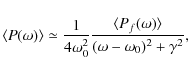
From the equation of a damped harmonic oscillator forced by a random
function, the average power of the Fourier transform of the
displacement can be approximated as,
 |
(1) |
where Pf is the power of the Fourier transform of the forcing function, and
where
where
with b being the background noise (which is assumed to be locally white) and
2.1 Application of Bayes theorem
The Bayes' Theorem can be stated as follows:
where p(A | D, I) is the probability for some hypothesis A given the data D and the prior information I. Note that I is also called the posterior probability of A. p(A | I) is the prior probability of A, p(D | A, I) is the likelihood function, and p(D | I) is the global likelihood. The latter serves as a normalizing constant and ensures the total probability summed over all hypotheses equals one. An extensive introduction to this field and the relevant methods can be found in Gregory (2005).
In order to apply the Bayesian formulation to any problem, one has to identify and assign probabilities for the individual terms in Eq. (4). In the following subsections we discuss our choices.
2.2 The likelihood function
The statistic of a power spectrum is given by a ![]() distribution with 2 degrees of freedom. The probability density that a model spectrum m matches an observed power spectrum o corresponds to
distribution with 2 degrees of freedom. The probability density that a model spectrum m matches an observed power spectrum o corresponds to
where
2.3 The role of the priors - improving the MLE approach
The simplest model of a p-mode profile consists of four parameters: mode frequency, mode height, mode lifetime, and background offset. Physically, the mode height and mode lifetime parameters are correlated. However, here we refrain from using this information and assume them to be independent. This enables us to use the mode height parameter as a device to distinguish between a detection and a non-detection of p-mode signal. We define the following two priors, called ignorance priors because they make no assumptions about the physical properties of the object being modeled:
- 1.
- for a mode with frequency
 ,
mode lifetime
,
mode lifetime  ,
background offset b we assume a uniform prior of the form
,
background offset b we assume a uniform prior of the form
(6)
where x stands for the respective parameters,
,
and b.
That is, we assume that the probability is equal across the range of
parameters and makes obvious the nomenclature, ignorance prior. For the
prior of the frequency parameter this is an appropriate choice, since
we cannot a priori exclude, for an observed spectrum, any value
within the range defined by the upper and lower p-mode frequencies. The
mode lifetime and the background offset, as long as they do not vary
across the fitted part of the spectrum by more than a magnitude, are
mostly determined by the global properties of the power spectrum and
therefore also warrant a uniform prior;
- 2.
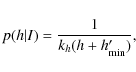
- for a mode with height h we adopt a modified Jeffrey's prior of the form
where
(8)
and (>0) expresses the ``strength'' of the prior. Lower values of
decrease the probability associated with
(>0) expresses the ``strength'' of the prior. Lower values of
decrease the probability associated with
 .
In contrast to the uniform prior, the Jeffrey's prior is normally
employed to ensure a uniform probability density per decade range
(e.g., the prior probability between 0.001 and 0.01 is the
same as between 0.01 and 0.1). The modified prior behaves
like a Jeffrey's prior for
.
In contrast to the uniform prior, the Jeffrey's prior is normally
employed to ensure a uniform probability density per decade range
(e.g., the prior probability between 0.001 and 0.01 is the
same as between 0.01 and 0.1). The modified prior behaves
like a Jeffrey's prior for
 ,
yet allows for values smaller than
.
In this regime it acts like a standard uniform prior and avoids a logarithm of 0.
,
yet allows for values smaller than
.
In this regime it acts like a standard uniform prior and avoids a logarithm of 0.
| (9) |
The ratio of the probabilities

is an odds ratio for the models ``mode height = h'' and ``mode height
If
To summarize, the mode height clearly is a scale parameter, rather than a location parameter (see Gregory 2005). Choosing
![]() allows one to set a lower limit for mode peak detection. The MLE
procedure does not implicitly allow for such a restriction and, thus,
makes it prone to overfitting.
allows one to set a lower limit for mode peak detection. The MLE
procedure does not implicitly allow for such a restriction and, thus,
makes it prone to overfitting.
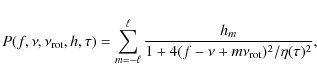
2.4 Treatment of rotational effects using ignorance priors
The effects of stellar rotation complicate the picture tremendously. If
rotational splitting is suspected, one can replace single Lorentzian
profiles with a sum of profiles. The central Lorentzian of the
rotationally split mode can be treated just like a single profile,
i.e., it has the same parameters and corresponding priors. The number
of suspected split components, however, depends on the spherical degree
of the mode. The components themselves are characterized by the
rotational splitting and their mode heights, which relative to each
other and the central peak depend on the stars inclination angle (see,
e.g., Gizon & Solanki 2003).
If the SNR conditions are very poor and/or a preliminary mode
identification is not possible, we chose not to use the inclination
angle as a parameter but to set the heights of the split components as
individual free parameters (see Eq. (3)).
Each Lorentzian profile in the model can a priori be ``equipped''
with a number of rotationally split components conforming to the
highest value of ![]() expected to be present in the data. The corresponding height priors,
then, only allow significant mode heights of those components in the
rotationally split multiplets for which there is enough evidence in the
data. This way, no preliminary mode identification is necessary. Alas,
using this approach the number of parameters needed for the model
increases tremendously. For high SNR data, where the degree of the
modes becomes even visually apparent through the rotational splitting,
a preliminary mode identification is certainly a more sensible
approach. In such a case, though, our method is not needed anyway.
expected to be present in the data. The corresponding height priors,
then, only allow significant mode heights of those components in the
rotationally split multiplets for which there is enough evidence in the
data. This way, no preliminary mode identification is necessary. Alas,
using this approach the number of parameters needed for the model
increases tremendously. For high SNR data, where the degree of the
modes becomes even visually apparent through the rotational splitting,
a preliminary mode identification is certainly a more sensible
approach. In such a case, though, our method is not needed anyway.
3 Application using MCMC
The analytic evaluation of complex models in a large parameter space in terms of Bayesian probability soon reaches the limit of computer resources. Stochastic methods can provide a sufficient sampling of the parameter regions of interest at a much smaller cost. In particular applications of the MCMC-technique have therefore gained increasing popularity and the (Bayesian) problems to which MCMC nowadays are applied range from the detection of planets (Gregory 2007), to the analysis of solar-type pulsators (Brewer et al. 2007), to spot modelling of active stellar atmospheres (Croll 2006).
Basically, MCMC performs a sequential walk through the parameter space of a specific problem. The MCMC technique probes solutions to the Bayesian equations by generating a random set of model parameters at some point and then progressing through parameter space via a biased random walk. This bias directing the chain of steps through parameter space is provided by the Bayesian probabilities themselves. Specifically, each parameter of the model is incremented or decremented by some random fraction of a predefined step width and the procedure then accepts or declines this combination of steps. The condition of acceptance is provided by the Metropolis-Hastings algorithm (Hastings 1970), which is based on the ratio of probabilities of subsequent parameter configurations before and after the step. In order to comply with this algorithm, the random steps do not necessarily have to be sampled from a symmetric proposal distribution. However, using such a distribution (uniform, Gaussian, etc.) is more intuitive and facilitates the necessary calibration of the algorithm (see below). MCMC scales with an increasing number of parameters and it is an ideal tool for solving our problem. We note that the Metropolis-Hastings algorithm evaluates only the relative probability between different parameter configurations. The normalisation factor of Eq. (4), which is often very difficult to evaluate, does not need to be calculated and will be dropped here after.
3.1 Semi-automated MCMC calibration
In order for the MCMC-implementation to operate efficiently the acceptance rate must be properly calibrated. When there are more than two parameters it can be shown that the acceptance rate should be about 0.25 in order to minimize correlations between the different parameters (Roberts et al. 1997). Because the acceptance rate depends mainly on the step width of each parameter, the step widths, themselves, have to be calibrated. The calibration process becomes more and more cumbersome as the number of parameters increases. We, therefore, implemented the following automated MCMC calibration scheme, similar to that described in Gregory (2005).
Given an observed power spectrum, several non-overlapping frequency
windows are defined that envelope the range of the individual mode
frequency parameters. The number of Lorentzian profiles to be
investigated per window is specified, and the lower and upper
constraints for the mode height(s), the mode lifetime(s), etc. are
defined. The model spectrum is initialized with appropriate starting
parameters, such as equidistant frequencies within the frequency
windows and mean values for the mode height, mode lifetime, and so on.
The MCMC algorithm is started with a step width of
| (12) |
for each model parameter x, where
Once the desired individual acceptance rates remain fairly stable, our algorithm switches to the standard MCMC routine, where the probability of a new configuration, and therefore the probability of its acceptance, is evaluated after all parameters have been slightly changed according to a random walk. At this point the MCMC routine is set to automatically test the parameter space.
3.2 Evaluating the MCMC results
Since the acceptance probability for each step is calculated using the Bayesian posterior probability, the MCMC routine will compute distributions (marginal distributions) for each involved parameter. After a sufficient number of iterations the marginal distributions for all model frequencies, mode heights, mode lifetimes, and background offsets can be estimated from histograms that count how frequently respective values of each parameter were visited. An estimate for the validity of the tested model can be obtained by examining these distributions.If any strong asymmetries, multiple local maxima, and other obviously non-Gaussian features appear they can be used to guide one toward an improved model. Regardless, the uncertainties for all parameters can be obtained from the cumulative distribution function of the normalized histograms.
4 Simulations
In order to test our method with parameters similar to a typical CoRoT run we generated 100 time series of 60 days duration each following the procedure in Chaplin et al. (1997). Each simulated data run represents a different realisation of the signal described in Table 1.
Table 1: Input parameters for the simulated solar-type pulsator.
We calculated the power spectra of each time series and applied our Bayesian analysis. The frequency range was between 130 andTable 2:
Parameter limits for the analysis of the simulated solar-type pulsator. According to Eq. (7),
![]() was set to 10-6.
was set to 10-6.
![\begin{figure}
\par\includegraphics[width=8.5cm,clip]{11203fg1.eps}
\end{figure}](/articles/aa/full_html/2009/41/aa11203-08/img52.png) |
Figure 1: Results of the Bayesian analysis for one of the 100 simulated data sets. Upper panel: a) the power density spectrum calculated from the simulated data (dashed line) and the most probable model spectrum derived from the analysis (solid line); b) the marginal distributions of the mode frequency parameters for both Lorentzian profiles of the model. Middle panel: the corresponding marginal distributions of the mode height parameters. Dashed and solid lines refer to the respective distributions presented in the top panel b). Bottom panel: the marginal distribution of the mode lifetime parameter. |
| Open with DEXTER | |
4.1 Evaluation of the simulations
Figure 1 shows a
typical power spectrum calculated from one of the 100 test data
sets, along with the most probable fit to the data. All input parameter
values fall within the borders of the derived marginal distributions.
We present the median values for all the parameters (but see discussion
in Gregory 2005) and, importantly, the uncertainties. A closer inspection of Fig. 1 reveals that not all the derived parameter values fall within the 1![]() uncertainties of the parameter values of the simulated data. Indeed,
all the parameters for this example are underestimated: the median of
the f1 distribution deviates from the input value by 2.99
uncertainties of the parameter values of the simulated data. Indeed,
all the parameters for this example are underestimated: the median of
the f1 distribution deviates from the input value by 2.99![]() .
The corresponding mode height is underestimated by 0.37
.
The corresponding mode height is underestimated by 0.37![]() .
f2 is underestimated by 0.63
.
f2 is underestimated by 0.63![]() ,
with the corresponding mode height deviating by 1.2
,
with the corresponding mode height deviating by 1.2![]() .
The mode lifetime also deviates by 0.84
.
The mode lifetime also deviates by 0.84![]() .
Such deviations are expected and are a direct consequence of the stochastic nature of the signal.
.
Such deviations are expected and are a direct consequence of the stochastic nature of the signal.
![\begin{figure}
\par\includegraphics[width=8.5cm,clip]{11203fg2.eps}
\end{figure}](/articles/aa/full_html/2009/41/aa11203-08/img53.png) |
Figure 2:
Right panels: distribution of the derived median mode parameter values (
|
| Open with DEXTER | |
Figure 2 shows the
results for all 100 simulations. The median values derived from our
analysis are compared to the simulation input values and are plotted
against the corresponding normalized probabilities of these input
values, evaluated via the marginal distributions. As expected, the
input values are not always reproduced to within 1![]() (p > 0.682), but are consistently found within 3
(p > 0.682), but are consistently found within 3![]() .
The scatter of the derived median values of the parameters around the
input values behaves as expected. The median of the frequency parameter
is shown to be distributed symmetrically, while the mode lifetime and
mode heights follow a log-normal distribution. The figure also
illustrates the overall accuracy with which each parameter can be
reproduced. The frequency parameter shows a lower accuracy limit of
about
.
The scatter of the derived median values of the parameters around the
input values behaves as expected. The median of the frequency parameter
is shown to be distributed symmetrically, while the mode lifetime and
mode heights follow a log-normal distribution. The figure also
illustrates the overall accuracy with which each parameter can be
reproduced. The frequency parameter shows a lower accuracy limit of
about ![]() .
The corresponding lower limits for the mode height and mode lifetime parameters are much larger at about
.
The corresponding lower limits for the mode height and mode lifetime parameters are much larger at about ![]() .
.
In addition, Fig. 2 shows cumulative histograms for the parameter value probabilities of the evaluated simulations. These histograms indicate that the scatter of the probabilities of the input values, for individual realisations, can be roughly approximated by a normal distribution. As the derived marginal distributions for all parameters provide a consistent picture, we argue that the probability densities obtained from a single data set can be trusted.
4.2 The importance of the mode height prior
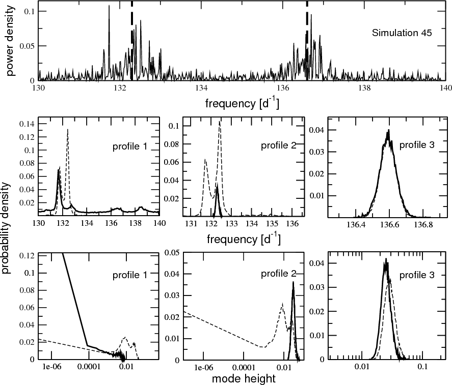 |
Figure 3:
3 Lorentzian profiles are fitted to simulated data that contain
2 frequencies. Top panel: power density spectrum of one of the
100 simulations mentioned in Sect. 4. The 2 input frequencies are marked by thick dashed lines. Additional power at |
| Open with DEXTER | |
As was argued in Sect. 2.3,
the mode height prior in its given form allows one to adjust the
fitting to better account for noise. The simulations described in the
previous Section provide us with an excellent example for this
rationale. In Fig. 3 we
show one of the simulations that includes by chance an additional power
excess in the frequency range of consideration due to noise and/or the
stochastic nature of the input signal. Using these data we tested how
looking for of a (non-existent) third Lorentzian profile would be
influenced by the
![]() parameter of the mode height prior. We evaluated the probabilities for
the existence of 3 Lorentzian profiles in the spectrum and
performed the analysis with two different values of
parameter of the mode height prior. We evaluated the probabilities for
the existence of 3 Lorentzian profiles in the spectrum and
performed the analysis with two different values of
![]() and
and
![]() .
The weaker prior with
.
The weaker prior with
![]() failed to correctly identify the noise peak as noise. This is similar
to the behavior of the MLE method, or any Bayesian application that
does not implicitly treat the problem of over-fitting due to, e.g.,
noise. The strong prior with
failed to correctly identify the noise peak as noise. This is similar
to the behavior of the MLE method, or any Bayesian application that
does not implicitly treat the problem of over-fitting due to, e.g.,
noise. The strong prior with
![]() ,
correctly distinguished between the noise peak and the two real profiles (see Fig. 3) and, in fact, determined a maximum in probability for a mode height of zero for the third.
,
correctly distinguished between the noise peak and the two real profiles (see Fig. 3) and, in fact, determined a maximum in probability for a mode height of zero for the third.
In the case of the strong prior, the marginal distribution of the frequency parameters for profile 2 and profile 3 are good approximations to a normal distribution and match the two input frequencies. Indeed, profile 2 is not influenced by the additional power excess in its vicinity. Although the marginal distribution shows a maximum probability for the frequency parameter at the location of the additional power excess, the marginal distribution also assigns significant probability densities to the whole parameter range. But more to the point the marginal distributions for the height prior, which again are well-shaped for profile 2 and profile 3, show a most probable mode height of zero for profile 1. That is, the profile 1 is unnecessary to fitting this range of frequencies with only two profiles are clearly detected.
In the case of the weak prior, the marginal distributions of the
frequency and mode height parameters of profile 1 and profile 2
intersect and mix. Hence, there seems to be evidence for a third
Lorentzian profile which is comparably strong to the evidence for the
actual Lorentzian profile at
![]() .
Moreover, profile 1 and profile 2 cannot be easily separated.
Thus, their mode parameters cannot be unambiguously determined. In
summary, with a weak mode-height prior (mimicking MLE methods) a third
mode is detected where none exist and the near by mode information is
distorted.
.
Moreover, profile 1 and profile 2 cannot be easily separated.
Thus, their mode parameters cannot be unambiguously determined. In
summary, with a weak mode-height prior (mimicking MLE methods) a third
mode is detected where none exist and the near by mode information is
distorted.
5 Application to the CoRoT target HD 49933
![\begin{figure}
\par\includegraphics[width=9cm]{11203fg4.eps}
\end{figure}](/articles/aa/full_html/2009/41/aa11203-08/img58.png) |
Figure 4:
Top panel: power density spectrum of HD 49933. Light grey:
original power density spectrum; dark grey: the original spectrum
smoothed with a 20 |
| Open with DEXTER | |
The question of detecting Lorentzian profiles is only relevant for data sets, where the SNR is high enough to see evidence for solar-type pulsation, but low enough to be questionably tractable with methods used in helioseismology. The ground-braking CoRoT data have all the qualities necessary for the technique to work:
- 1.
- good data quality devoid of strong instrumental signal or aliasing;
- 2.
- clear indication of Lorentzian profiles at least in the region of maximum pulsation power;
- 3.
- increasingly poor S/R further away from the region of maximum pulsation power.
Intrinsic stellar noise-like signal, mainly due to turbulent
convection, generates significant power in the frequency range of
pulsation and effects the accurate determination of mode parameters.
For the Sun Harvey (1985) modeled the background signal with a sum of power laws. Aigrain et al. (2004), and more recently Michel et al. (2009), use
![]() ,
with
,
with
![]() ,
or hereafter
,
or hereafter
![]() ,
to model the solar granulation signal, where
,
to model the solar granulation signal, where ![]() is the frequency,
is the frequency, ![]() is the characteristic times scale of the ith component and Ci is the slope of the power law. The normalisation factor ai is chosen such that
is the characteristic times scale of the ith component and Ci is the slope of the power law. The normalisation factor ai is chosen such that
![]() corresponds to the variance of the stochastic signal in the time
series. Whereas the slope of the power laws was arbitrary fixed
to 2 in Harvey's original model, Appourchaux et al. (2002) were the first to suggest a different value. Recently, Aigrain et al. (2004) and Michel et al. (2009)
have shown that, at least for the Sun, the slope is closer to 4.
Each power law represents a different physical process with time scales
for the Sun ranging from minutes in the case of granulation to days in
the case of stellar activity.
corresponds to the variance of the stochastic signal in the time
series. Whereas the slope of the power laws was arbitrary fixed
to 2 in Harvey's original model, Appourchaux et al. (2002) were the first to suggest a different value. Recently, Aigrain et al. (2004) and Michel et al. (2009)
have shown that, at least for the Sun, the slope is closer to 4.
Each power law represents a different physical process with time scales
for the Sun ranging from minutes in the case of granulation to days in
the case of stellar activity.
Appourchaux et al. (2008) used a single power
law for the background signal in the frequency range of pulsation and
fitted the corresponding parameters simultaneously with the p-mode
parameters to the observed power density spectrum. We have separated
the analysis of the background signal from the analysis of the
pulsation signal, in which case one has to model the pulsation signal
in the power density spectrum with a dedicated term in the global
background fit.
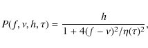
Kallinger et al. (2008) have shown that the
power excess hump due to pulsation can be approximated by a Gaussian
function. Hence, our global model to fit the heavily smoothed power
density spectrum of HD 49933 consists of a superposition of white
noise, three power law components, and a power excess hump approximated
by a Gaussian function:
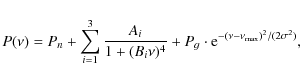
where Pn is the white noise component, Ai and Bi are the amplitudes and characteristic time scales of the power laws, Pg,
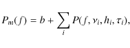
5.1 MCMC analysis
The frequency range between the lower and upper limits beyond which we see the pulsation signal disappearing in the noise was subdivided into 16 windows. To each, a chosen number of Lorentzian profiles was fitted, based on our Bayesian algorithm. The model parameters are presented in Table 4. This subdivision into windows was only chosen to accelerate the burn-in phase. It has no influence on the results, as long as the resulting marginal distributions for the mode frequency parameters are not intersected by the window borders. Yet, it still enables us to perform a global fit which includes the influence of Lorentzian profiles also from adjacent windows.
Table 3: Global fit parameters.
Table 4:
Parameter limits for the analysis of HD 49933. The height prior parameter was set to
![]() .
.
For the first analysis we decided to consider only 2 Lorentzian profiles in each window. Moreover, we also kept the mode lifetime uniform for all Lorentzian profiles, expecting that the marginal distribution of this parameter would tell us whether this assumption is valid.
![\begin{figure}
\par\includegraphics[width=17cm]{11203fg5.eps}
\end{figure}](/articles/aa/full_html/2009/41/aa11203-08/img69.png) |
Figure 5: Observed power density spectrum (gray) and fitted Lorentzian profiles. Vertical lines indicate the borders of the fitting windows (see text). The dashed lines in the bottom panel show two profiles for which our Bayesian technique results in ambiguous frequency distributions ranging over the whole fitting window |
| Open with DEXTER | |
Figure 5 shows the
power density spectrum, on which our analysis is based, together with
the fitting windows we defined, and the most probable model derived
after ![]() 1.3 million
iterations. The model manages to reproduce the observations quite well,
and there remain only very few frequency ranges where a visual
inspection seems to indicate additional power.
Beyond
1.3 million
iterations. The model manages to reproduce the observations quite well,
and there remain only very few frequency ranges where a visual
inspection seems to indicate additional power.
Beyond
![]() several Lorentzian profiles are fitted with fairly well defined
frequencies, but with a probability maximum for a mode height of zero.
Two profiles, listed in Table 5
as P25 and P26, indicated in the figure by dashed lines, have
ambiguous frequency distributions ranging over the whole fitting
window. What is shown is a biased choice to fit the general picture.
several Lorentzian profiles are fitted with fairly well defined
frequencies, but with a probability maximum for a mode height of zero.
Two profiles, listed in Table 5
as P25 and P26, indicated in the figure by dashed lines, have
ambiguous frequency distributions ranging over the whole fitting
window. What is shown is a biased choice to fit the general picture.
![\begin{figure}
\par\includegraphics[width=8cm,clip]{11203fg6.eps}
\end{figure}](/articles/aa/full_html/2009/41/aa11203-08/img71.png) |
Figure 6:
Top panel: marginal distribution of the mode frequency
parameter of one of the profiles fitted to the CoRoT data. The median
value, and the lower and upper 1 |
| Open with DEXTER | |
Figure 6 presents an example for the marginal frequency distribution and mode height for one of the Lorentzian profiles. As expected, the former can be very well approximated by a Gaussian, while the latter follows a log-normal distribution. The bottom panel shows a quite narrow and smooth mode height distribution for a simultaneous fit to all Lorentzian profiles, indicating a constant mode lifetime. The data therefore do not seem to warrant different mode lifetimes. It is thus save to assume that any variations among the various profiles for this parameter are accounted for within the uncertainty given by the mode lifetime distribution. Surprisingly, we do not find well-defined multi-modal distributions for any of the frequency parameters involved. Some ambiguities in the distributions are only apparent at very high frequencies and with the poorest SNR. Additional profiles, either due to modes of higher degree or rotational splitting, still could be present, if the frequencies are very well separated.
![\begin{figure}
\par\includegraphics[width=8cm,clip]{11203fg7.eps}
\end{figure}](/articles/aa/full_html/2009/41/aa11203-08/img72.png) |
Figure 7: Top panel: a) the fitted region in the power density spectrum, where the p modes have the highest SNR. The most probable model (thick solid line) is presented in comparison to the observations (dotted line). The borders of the fitting windows are indicated by the thick dashed lines. b) The marginal mode frequency distributions for 3 profiles per window. Six profiles are identified (black), while the additional profiles are ambiguous across the whole frequency range (gray lines). Frequencies identified by Appourchaux et al. (2008) are shown as thin dashed lines. Bottom panel: the corresponding mode height distributions. |
| Open with DEXTER | |
5.2 On the evidence for  = 2 modes
We repeated our analysis for the region with the highest SNR, but
included for each fitting window a third Lorentzian profile in our
model. The results are shown in presented in Fig. 7.
The probability distributions for the additional profiles consistently
favours a mode height of zero. Moreover, the corresponding mode
frequency distributions only vaguely contain regions of higher
probability. We therefore conclude that, based on our conservative
approach, any additional power in the power density spectrum is due to
noise or to the stochastic nature of the clearly detected modes. From
our perspective, focussing on the ``detection'' of profiles, the data
do not present convincing evidence for ![]() modes.
modes.
5.3 On the evidence for rotational splitting
The failed detection of additional profiles, and the single-mode nature
of the frequency distributions of detected profiles, suggests that the
effects expected from rotational splitting can most likely be neglected
in the analysis of the CoRoT data of HD 49933. Nonetheless, in
order to perform a more rigorous test, we analysed the same frequency
region shown in Fig. 7
including these effects. Our model used 2 Lorentzian profiles per
fitting window, each of which contains 2 additional features
corresponding to rotational splitting of ![]() modes (see Eq. (3)). Accordingly, a new global parameter, the rotation frequency, was introduced. Appourchaux et al. (2008) report the detection of a particular spectral feature at 3.4
modes (see Eq. (3)). Accordingly, a new global parameter, the rotation frequency, was introduced. Appourchaux et al. (2008) report the detection of a particular spectral feature at 3.4 ![]() Hz
which apparently corresponds to the HD 49933's rotation frequency.
We therefore used this value as a reference and allowed a scatter of
about 0.2
Hz
which apparently corresponds to the HD 49933's rotation frequency.
We therefore used this value as a reference and allowed a scatter of
about 0.2 ![]() Hz in either direction. This range corresponds to twice the classical frequency resolution
Hz in either direction. This range corresponds to twice the classical frequency resolution
![]() of the CoRoT time series, where
of the CoRoT time series, where ![]() is the length of the data set, and was used to define the borders of a
uniform prior. The heights of the rotation profiles were implemented as
usual, using modified Jeffrey's priors for these parameters. We
expected a well defined distribution for the rotation frequency to
emerge from the analysis. However, we find no preferred value for this
parameter, as is shown in Fig. 8. The distribution is mostly consistent with sampling noise.
is the length of the data set, and was used to define the borders of a
uniform prior. The heights of the rotation profiles were implemented as
usual, using modified Jeffrey's priors for these parameters. We
expected a well defined distribution for the rotation frequency to
emerge from the analysis. However, we find no preferred value for this
parameter, as is shown in Fig. 8. The distribution is mostly consistent with sampling noise.
Concerning the mode heights, alternating detections and non-detections
of the rotation profiles would indicate a difference in their central
profiles between radial and non-radial modes. We cannot find any such
differences, since the mode height distributions for the rotation
profiles are consistent with a null result. While the star certainly
does rotate, it seems that the signal is too close to the noise level
to support any need for these parameters. In other words, rotational
effects, if present, seem to be ill-defined and do not need to be
considered for the frequency analysis of this data set. As an example
of a near ideal case, the bottom panel of Fig. 8
shows corresponding results from a single mode using 60 days of
data of the Sun observed as a star by the VIRGO (green band) instrument
on board the SOHO spacecraft (see Fröhlich et al. 1997, and references therein). Fitting only the small range between 3090 and 3110 ![]() Hz and using the same profile model as for HD 49933, the rotational splitting becomes apparent.
Hz and using the same profile model as for HD 49933, the rotational splitting becomes apparent.
![\begin{figure}
\par\includegraphics[width=8cm]{11203fg8.eps}
\end{figure}](/articles/aa/full_html/2009/41/aa11203-08/img77.png) |
Figure 8: Top panel: the marginal distribution of the rotational splitting parameter derived as explained in Sect. 5.3. The thick black line is a boxcar average using 10 data points. Bottom panel: the same but for the analysis of VIRGO data of the Sun. |
| Open with DEXTER | |
5.4 Results
As a consequence of the results from the previous two sections, we use
only 2 modes per window without any rotational splitting for our
global fit. For 6 of the 32 fitted profiles, the
identification is ambiguous (or the most probable mode heights are
close to zero) due to the low SNR. All other profiles are clearly
detected and their parameters have smooth, single-mode distributions.
The results of our analysis are presented in Table 5. The 1![]() -errors
have been derived from the cumulative distribution functions, which are
evaluated using the marginal distributions for all parameters. We find
that the data are consistent with a mode lifetime of roughly
0.5 days which does not appear to vary significantly across the
spectrum. The confidence for this overall result can be calculated via
the mode height parameter. As we have used
-errors
have been derived from the cumulative distribution functions, which are
evaluated using the marginal distributions for all parameters. We find
that the data are consistent with a mode lifetime of roughly
0.5 days which does not appear to vary significantly across the
spectrum. The confidence for this overall result can be calculated via
the mode height parameter. As we have used
![]() ,
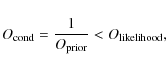
the result gives an odds ratio condition
,
the result gives an odds ratio condition
![]() .
.
Therefore, the obtained parameter distributions are at least
![]() times
more probable than a model spectrum that only consists of the
background offset. The profiles 25 and 26 are only listed for
sake of completeness. Due to the ambiguity in their marginal frequency
distribution, apparent in their given uncertainties, we do not assign
credibility to these values. The final Echelle diagram is displayed in
Fig. 9. The frequencies estimated as
times
more probable than a model spectrum that only consists of the
background offset. The profiles 25 and 26 are only listed for
sake of completeness. Due to the ambiguity in their marginal frequency
distribution, apparent in their given uncertainties, we do not assign
credibility to these values. The final Echelle diagram is displayed in
Fig. 9. The frequencies estimated as ![]() by Appourchaux et al. (2008) agree very well with our corresponding values, and the 1
by Appourchaux et al. (2008) agree very well with our corresponding values, and the 1![]() -uncertainties
are comparable in both studies. The remaining frequencies, however,
differ due to the cited authors' explicit assumption of
-uncertainties
are comparable in both studies. The remaining frequencies, however,
differ due to the cited authors' explicit assumption of ![]() modes, which we do not detect.
modes, which we do not detect.
Although we deliberately did not include fixed mode height ratios for
modes of different degree in our model, the resulting mode height
ratios are mostly consistent within the uncertainties with a fixed
ratio. The obvious outlier in Fig. 10 at ![]()
![]() is due to profiles 25 and 26, which we already marked as highly suspicious.
is due to profiles 25 and 26, which we already marked as highly suspicious.
Table 5: Results of the CoRoT data for HD 49933.
![\begin{figure}
\par\includegraphics[width=7.5cm,clip]{11203fg9.eps}
\end{figure}](/articles/aa/full_html/2009/41/aa11203-08/img86.png) |
Figure 9: Echelle diagram showing the identified frequencies (solid error bars). Values belonging to profile 25 and 26 (see Table 5) are indicated by the dashed error bars. Frequencies found by Appourchaux et al. (2008) are displayed in grey. |
| Open with DEXTER | |
![\begin{figure}
\par\includegraphics[width=8.4cm,clip]{11203fg10.eps}
\end{figure}](/articles/aa/full_html/2009/41/aa11203-08/img87.png) |
Figure 10:
The mode height ratios for subsequent modes listed in Table 5 (e.g.,
hP2/hP1) are shown as filled circles. The dotted lines correspond to the |
| Open with DEXTER | |
6 Discussion
With high quality data and evidence for additional and/or closely spaced modes, such as might appear for nonradial modes split by rotation, we believe that it might be advantageous to change the peak Lorentzian model by combining the corresponding Lorentzian profiles and fitting them as a group. Eventually, once the quality of the data becomes even better, we think that a more classical Bayesian treatment replacing the ignorance priors with specific information from theory or previous observations, is more appropriate because the potential gain in information outweighs the danger of over-fitting. Benomar (2008) has performed such an analysis for the data set also presented in this paper, and obviously obtained different results. It thus remains questionable whether the Initial Run CoRoT data of HD 49933 is already good enough for such an approach.![\begin{figure}
\par\includegraphics[width=8cm,clip]{11203fg11.eps}
\end{figure}](/articles/aa/full_html/2009/41/aa11203-08/img88.png) |
Figure 11: The high-frequency region devoid of p-mode signal used for testing the global likelihood comparison. Note that the scale is similar to Fig. 5. |
| Open with DEXTER | |
6.1 On the global likelihood of p-mode profiles
In this paper we have used Bayes' theorem to solve a parameter estimation problem. One of the biggest advantages of Bayesian analysis, however, is to perform model comparison. This is achieved by first calculating the global likelihood via integration over all model parameters. The global likelihoods are subsequently used to compare the different models themselves. It would be interesting to use parallel tempering (e.g., Benomar 2008), an algorithm which allows the Markov chain to more easily sample the complete parameter space, to perform such model selection by calculating the global likelihood of a model via integration over the tempering parameter (see, e.g., Gregory 2007). However, we think that the validity of applying this kind of model selection to p-mode analysis needs to be carefully tested first.
As a first trial run, we have investigated how the global likelihood of
three simple models behaves in a region of pure noise. We studied the
region between 4600 and 4700 ![]() Hz in the power spectrum of HD 49933 (see Fig. 11)
which is far beyond the region of pulsation. At such high frequencies,
the power spectrum should be dominated by the noise properties of the
instrument. Following the description given in Gregory (2005) on how to obtain the global likelihood, we evaluated three models
Hz in the power spectrum of HD 49933 (see Fig. 11)
which is far beyond the region of pulsation. At such high frequencies,
the power spectrum should be dominated by the noise properties of the
instrument. Following the description given in Gregory (2005) on how to obtain the global likelihood, we evaluated three models
- M1: constant noise level;
- M2: constant noise level + 1 Lorentzian profile; and
- M3: constant noise level + 2 Lorentzian profiles.
Depending on the choice of the tempering parameters used in the parallel tempering process, as well as on differences in the numerical integration scheme required to calculate these numbers, the end result varies, but the overall magnitudes of difference in probability remain the same. The likelihood function alone seems to prefer models with (more) Lorentzian profiles, even if there are none (related to solar-type oscillations) present in the data.
This is an issue demanding clarification. It will be required to test the influence of the allowed parameter ranges in order to see where this preference arises in the integration over the parameter space. Moreover, the influence from different kind of prior probabilities on the global likelihoods also needs to be studied. To conclude, our initial test suggests that we cannot yet trust the global likelihood completely when comparing models of power spectra (to real data at least) until we are able to clarify this issue.
7 Conclusion
We have presented a conservative approach (using only ignorance priors) for a Bayesian analysis of solar-type p modes with a minimum of parameters. The method uses a mode-height prior that allows us to more easily and reliably distinguish real peaks from those that arise stochastically from noise, in reference to a threshold set by the user. We show how the marginal distributions of all the parameters can be obtained. Our tests with simulated data succeeded by reproducing the simulation input values and not being confused by randomly occurring noise peaks. Furthermore, we have applied our method to the Initial Run CoRoT data of HD 49933, where we can easily and unambiguously identify at least 26 p modes. We fail to detectWe would like to especially thank Daniel Huber (Sydney Institute for Astronomy, Sydney, Australia) for interesting discussions. We also thank Peter Reegen (Institute for Astronomy, Vienna, Austria) and Tim Bedding (Sydney Institute for Astronomy, Sydney, Australia) for their suggestions. M.G., T.K. and W.W. have received financial support by the Austrian Fonds zur Förderung der wissenschaftlichen Forschung (P17890-N02). D.B.G. acknowledges funding from the Natural Sciences & Engineering Research Council (NSERC) Canada. Last but not least, we are very thankful for the constructive comments provided by the anonymous referee who helped to greatly improve this article. We are grateful for the VIRGO data being publicly available.
References
- Aigrain, S., Favata, F., & Gilmore, G. 2004, A&A, 414, 1139 [NASA ADS] [CrossRef] [EDP Sciences]
- Appourchaux, T. 2008, Astron. Nachr., 329, 485 [NASA ADS] [CrossRef]
- Appourchaux, T., Gizon, L., & Rabello-Soares, M.-C. 1998, A&AS, 132, 107 [NASA ADS] [CrossRef] [EDP Sciences]
- Appourchaux, T., Andersen, B., & Sekii, T. 2002, in From Solar Min to Max: Half a Solar Cycle with SOHO, ed. A. Wilson, ESA SP, 508, 47
- Appourchaux, T., Michel, E., Auvergne, M., et al. 2008, A&A, 488, 705 [NASA ADS] [CrossRef] [EDP Sciences]
- Baglin, A., Michel, E., Auvergne, M., et al. 2006, in ESA SP, 1306, 39
- Bedding, T., & Kjeldsen, H. 2006, in Proceedings of SOHO 18/GONG 2006/HELAS I, Beyond the spherical Sun, ESA SP, 624
- Benomar, O. 2008, Commun. Asteroseismol., 157, 98 [NASA ADS]
- Brewer, B. J., Bedding, T. R., Kjeldsen, H., & Stello, D. 2007, ApJ, 654, 551 [NASA ADS] [CrossRef]
- Chaplin, W. J., Elsworth, Y., Howe, R., et al. 1997, MNRAS, 287, 51 [NASA ADS]
- Croll, B. 2006, PASP, 118, 1351 [NASA ADS] [CrossRef]
- Fröhlich, C., Crommelynck, D. A., Wehrli, C., et al. 1997, Sol. Phys., 175, 267 [NASA ADS] [CrossRef]
- Gizon, L., & Solanki, S. K. 2003, ApJ, 589, 1009 [NASA ADS] [CrossRef]
- Gregory, P. C. 2005, Bayesian Logical Data Analysis for the Physical Sciences: a Comparative Approach with ``Mathematica'' Support, ed. P. C. Gregory (Cambridge, UK: Cambridge University Press)
- Gregory, P. C. 2007, MNRAS, 374, 1321 [NASA ADS] [CrossRef]
- Harvey, J. 1985, in Future Missions in Solar, Heliospheric & Space Plasma Physics, ed. E. Rolfe, & B. Battrick, ESA SP, 235, 199
- Hastings 1970, Biometrika, 57, 97 [CrossRef]
- Kallinger, T., Weiss, W. W., Barban, C., et al. 2008, A&A, submitted
- Kallinger, T., Gruberbauer, M., Guenther, D. B., Fossati, L., & Weiss, W. W. 2009, [arXiv:0811.4686]
- Michel, E., Samadi, R., Baudin, F., et al. 2009, A&A, 495, 979 [NASA ADS] [CrossRef] [EDP Sciences]
- Roberts, G. O., Gelman, A., & Gilks, W. R. 1997, Ann. Appl. Prob., 7, 110 [CrossRef]
- Toutain, T., & Appourchaux, T. 1994, A&A, 289, 649 [NASA ADS]
Footnotes
- ... CoRoT
![[*]](/icons/foot_motif.png)
- The CoRoT (COnvection, ROtation and planetary Transits space mission, launched on 2006 December 27, was developed and is operated by the CNES, with participation of the Science Programs of ESA, ESAs RSSD, Austria, Belgium, Brazil, Germany and Spain.
All Tables
Table 1: Input parameters for the simulated solar-type pulsator.
Table 2:
Parameter limits for the analysis of the simulated solar-type pulsator. According to Eq. (7),
![]() was set to 10-6.
was set to 10-6.
Table 3: Global fit parameters.
Table 4:
Parameter limits for the analysis of HD 49933. The height prior parameter was set to
![]() .
.
Table 5: Results of the CoRoT data for HD 49933.
All Figures
| |
Figure 1: Results of the Bayesian analysis for one of the 100 simulated data sets. Upper panel: a) the power density spectrum calculated from the simulated data (dashed line) and the most probable model spectrum derived from the analysis (solid line); b) the marginal distributions of the mode frequency parameters for both Lorentzian profiles of the model. Middle panel: the corresponding marginal distributions of the mode height parameters. Dashed and solid lines refer to the respective distributions presented in the top panel b). Bottom panel: the marginal distribution of the mode lifetime parameter. |
| Open with DEXTER | |
| In the text | |
| |
Figure 2:
Right panels: distribution of the derived median mode parameter values (
|
| Open with DEXTER | |
| In the text | |
| |
Figure 3:
3 Lorentzian profiles are fitted to simulated data that contain
2 frequencies. Top panel: power density spectrum of one of the
100 simulations mentioned in Sect. 4. The 2 input frequencies are marked by thick dashed lines. Additional power at |
| Open with DEXTER | |
| In the text | |
| |
Figure 4:
Top panel: power density spectrum of HD 49933. Light grey:
original power density spectrum; dark grey: the original spectrum
smoothed with a 20 |
| Open with DEXTER | |
| In the text | |
| |
Figure 5: Observed power density spectrum (gray) and fitted Lorentzian profiles. Vertical lines indicate the borders of the fitting windows (see text). The dashed lines in the bottom panel show two profiles for which our Bayesian technique results in ambiguous frequency distributions ranging over the whole fitting window |
| Open with DEXTER | |
| In the text | |
| |
Figure 6:
Top panel: marginal distribution of the mode frequency
parameter of one of the profiles fitted to the CoRoT data. The median
value, and the lower and upper 1 |
| Open with DEXTER | |
| In the text | |
| |
Figure 7: Top panel: a) the fitted region in the power density spectrum, where the p modes have the highest SNR. The most probable model (thick solid line) is presented in comparison to the observations (dotted line). The borders of the fitting windows are indicated by the thick dashed lines. b) The marginal mode frequency distributions for 3 profiles per window. Six profiles are identified (black), while the additional profiles are ambiguous across the whole frequency range (gray lines). Frequencies identified by Appourchaux et al. (2008) are shown as thin dashed lines. Bottom panel: the corresponding mode height distributions. |
| Open with DEXTER | |
| In the text | |
| |
Figure 8: Top panel: the marginal distribution of the rotational splitting parameter derived as explained in Sect. 5.3. The thick black line is a boxcar average using 10 data points. Bottom panel: the same but for the analysis of VIRGO data of the Sun. |
| Open with DEXTER | |
| In the text | |
| |
Figure 9: Echelle diagram showing the identified frequencies (solid error bars). Values belonging to profile 25 and 26 (see Table 5) are indicated by the dashed error bars. Frequencies found by Appourchaux et al. (2008) are displayed in grey. |
| Open with DEXTER | |
| In the text | |
| |
Figure 10:
The mode height ratios for subsequent modes listed in Table 5 (e.g.,
hP2/hP1) are shown as filled circles. The dotted lines correspond to the |
| Open with DEXTER | |
| In the text | |
| |
Figure 11: The high-frequency region devoid of p-mode signal used for testing the global likelihood comparison. Note that the scale is similar to Fig. 5. |
| Open with DEXTER | |
| In the text | |
Copyright ESO 2009
Current usage metrics show cumulative count of Article Views (full-text article views including HTML views, PDF and ePub downloads, according to the available data) and Abstracts Views on Vision4Press platform.
Data correspond to usage on the plateform after 2015. The current usage metrics is available 48-96 hours after online publication and is updated daily on week days.
Initial download of the metrics may take a while.