| Issue |
A&A
Volume 506, Number 1, October IV 2009
The CoRoT space mission: early results
|
|
|---|---|---|
| Page(s) | 435 - 444 | |
| Section | Astronomical instrumentation | |
| DOI | https://doi.org/10.1051/0004-6361/200911906 | |
| Published online | 02 July 2009 | |
The CoRoT space mission: early results
Narrow frequency-windowed autocorrelations as a diagnostic of solar-like stars
I. W. Roxburgh1,2
1 - Queen Mary University of London, Astronomy Unit,
Mile End Road, London E1 4NS, UK
2 - LESIA, Observatoire de Paris, Place Jules Janssen, 92195 Meudon, France
Received 20 February 2009 / Accepted 17 June 2009
Abstract
Aims. This paper investigates the diagnostic potential of narrow, frequency-windowed autocorrelation as a tool for probing the properties of solar-like oscillating stars when the determination of individual frequencies is impossible or is subject to large uncertainties, and when mode identification is difficult.
Methods. I use theoretical analysis including phase-shifts, modelling, and data analysis.
Results. Narrow-windowed autocorrelation of a time series can reveal the variation with frequency of the large separations
![]() and the half large separations
and the half large separations
![]() ,
thus helping with mode identification. This technique is applied to the CoRoT p-mode oscillators HD 49933, HD 175726, HD 181420, and HD 181906. Theoretical analysis and modelling are presented to illustrate the technique.
,
thus helping with mode identification. This technique is applied to the CoRoT p-mode oscillators HD 49933, HD 175726, HD 181420, and HD 181906. Theoretical analysis and modelling are presented to illustrate the technique.
Key words: stars: oscillations - methods: analytical - methods: data analysis
1 Introduction
For solar-like stars reliable determining of p-mode frequencies from power spectra is not always possible since the amplitudes of the stochastically excited modes are very small, giving low signal/noise. For F stars observed by CoRoT![]() the line widths are large, which hinders the reliable determination of frequencies and for some stars, particularly HD 175726, individual frequencies are exceedingly difficult to extract.
I here consider an alternative approach that may be useful when faced with poor quality data, namely the use of the autocorrelation of the time series. As shown by Roxburgh & Vorontsov (2006a) by adding noise to a solar power spectrum, this has diagnostic potential when faced with noisy data.
the line widths are large, which hinders the reliable determination of frequencies and for some stars, particularly HD 175726, individual frequencies are exceedingly difficult to extract.
I here consider an alternative approach that may be useful when faced with poor quality data, namely the use of the autocorrelation of the time series. As shown by Roxburgh & Vorontsov (2006a) by adding noise to a solar power spectrum, this has diagnostic potential when faced with noisy data.
The autocorrelation of a discrete time series G(tk), k=0,N is
 |
(1) |
One can see immediately that peaks are expected in the autocorrelation function of a photometric time series due to p-mode oscillations. Such oscillations are acoustic waves excited by surface convection. A wave packet produced near the surface of the star propagates to the far side of the star in time 2T, where T is the acoustic radius of the star, and is reflected back arriving at (or near) the point of emission at 4T. Thus one expects a peak in the autocorrelation at
To concentrate on frequency components in the photometric time series of a star in the range of p-mode oscillations, one can filter the time series by transforming to the frequency domain, windowing the resulting Fourier transform to retain only contributions in a given frequency range, then transform back to the time domain and take the autocorrelation of the resulting time series.
From the Wiener-Khinchin theorem the autocorrelation A(t) is equal to the real part of the Fourier transform ![]() of the power spectrum
of the power spectrum ![]() of the time series, and the amplitude envelope
of the time series, and the amplitude envelope
![]() by the amplitude of the full Fourier transform:
by the amplitude of the full Fourier transform:
 |
(2) |
(cf. Press et al. 1992). It is therefore not necessary to transform back to the time domain but simply to take the Fourier transform of the filtered power spectrum. Figure 1 shows the autocorrelation and the amplitude envelope of the photometric time series of the F5V star HD 49933 observed for 60 days in the initial run of CoRoT (see below and Appourchaux et al. 2008), which has been filtered (using a
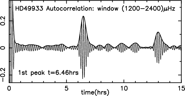 |
Figure 1:
HD 49933 autocorrelation, frequency windowed between
|
| Open with DEXTER | |
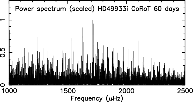 |
Figure 2: HD 49933 power spectrum. |
| Open with DEXTER | |
To determine the location of the peaks in the filtered autocorrelation function (Fig. 1),
one could fit a Gabor function to the rapidly oscillating autocorrelation (cf. Kholikov & Hill 2008), but it is more convenient to use the amplitude envelope or its square, the autocorrelation power. As mentioned above, the first peak in the autocorrelation is expected at 4T, where
![]() is the acoustic radius of the star, the time for a wave to travel from centre to surface (here c(r) is the sound speed), and this gives an estimate of the large separation
is the acoustic radius of the star, the time for a wave to travel from centre to surface (here c(r) is the sound speed), and this gives an estimate of the large separation ![]() .
However, as the actual ray path and the location of the reflecting layer in the atmosphere depend on the star's structure and on frequency and degree, the round trip travel time is not independent of
.
However, as the actual ray path and the location of the reflecting layer in the atmosphere depend on the star's structure and on frequency and degree, the round trip travel time is not independent of ![]() ,
and the large separations
,
and the large separations
![]() vary with both frequency and degree. This variation is primarily due to the quasi-periodic modulation of the frequencies caused by the HeII ionisation layer and to the different contributions of the inner layers to frequencies of different degree
vary with both frequency and degree. This variation is primarily due to the quasi-periodic modulation of the frequencies caused by the HeII ionisation layer and to the different contributions of the inner layers to frequencies of different degree ![]() .
Additionally there can be a small contribution at 2T due to reflection from the core (Roxburgh & Vorontsov 1996,7).
I here examine whether information on this variation with frequency and degree can be extracted from the autocorrelation power by narrow windowing in the frequency domain.
.
Additionally there can be a small contribution at 2T due to reflection from the core (Roxburgh & Vorontsov 1996,7).
I here examine whether information on this variation with frequency and degree can be extracted from the autocorrelation power by narrow windowing in the frequency domain.
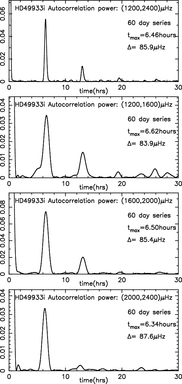 |
Figure 3:
Frequency windowed autocorrelation power for HD 49933 (scaled): a) windowed between
|
| Open with DEXTER | |
2 The CoRoT star HD 49933
The F5V (mv=5.77) star HD 49933 was observed for 60 days in the initial run of CoRoT (see Appourchaux et al. 2008). After applying several corrections, details of which are given in Samadi et al. (2006), the light curves are sampled at a cadence of 32 s, the duty cycle is ![]() 90% and the gaps, mainly due to the passages of the satellite through the South Atlantic anomaly, are filled by interpolation. (This is level 2 data in the language of CoRoT.) The typical length of the gaps is
90% and the gaps, mainly due to the passages of the satellite through the South Atlantic anomaly, are filled by interpolation. (This is level 2 data in the language of CoRoT.) The typical length of the gaps is ![]() 9 min, producing a
9 min, producing a ![]() 10% reduction in power at frequencies >2000
10% reduction in power at frequencies >2000 ![]() Hz (see Appourchauux et al. 2008).
Hz (see Appourchauux et al. 2008).
The resulting light curve has a mean drift and significant variations due to rotation and activity, this can be removed by subtracting off a running mean. Linear interpolation in the gaps can be modified by adding noise based on the mean variation outside the gaps.
Experiments using different running means, and none, and different gap-filling procedures showed that the results described below were independent of these procedures. The power spectrum
using the level 2 data is shown in Fig. 2 for the frequency range
![]() Hz.
Hz.
This power spectrum was then filtered with a ![]() window
window
![]() with
with
![]() Hz and the resulting autocorrelation (normalised to 1 at t=0) is that shown Fig. 1 above, and the autocorrelation power in Fig. 3a. The first peak occurs at a time
Hz and the resulting autocorrelation (normalised to 1 at t=0) is that shown Fig. 1 above, and the autocorrelation power in Fig. 3a. The first peak occurs at a time
![]() h corresponding to a mean large separation of
h corresponding to a mean large separation of ![]() Hz, the second peak at
Hz, the second peak at
![]() and a third peak can just be detected at
and a third peak can just be detected at
![]() .
The rapid decrease in the height of successive peaks in Fig. 3a indicates the short life time of the modes; this is to be expected since the line widths in the power spectrum are broad (Appourchaux et al. 2008).
.
The rapid decrease in the height of successive peaks in Fig. 3a indicates the short life time of the modes; this is to be expected since the line widths in the power spectrum are broad (Appourchaux et al. 2008).
Figures 3b-d show the autocorrelation power for three independent narrower windows of ![]() Hz. These again show the characteristic maxima near 6.46 h, but they are not at exactly at the same values. This suggests one may be able to extract more detailed information on the frequency variation of
Hz. These again show the characteristic maxima near 6.46 h, but they are not at exactly at the same values. This suggests one may be able to extract more detailed information on the frequency variation of ![]() by using such narrow windows.
by using such narrow windows.
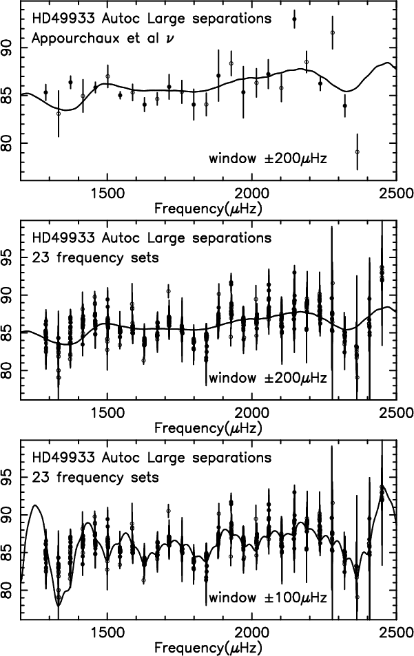 |
Figure 4:
a) Variation of large separation with frequency for HD 49933 from autocorrelation with a |
| Open with DEXTER | |
I then took a set of narrower windows of ![]() 200 Hz centred on a frequency
200 Hz centred on a frequency ![]() and moved the windows through the frequency range
and moved the windows through the frequency range
![]() Hz in steps of
Hz in steps of ![]() Hz, and determined the location of the peaks tk in the autocorrelation power near 6.46 h, and hence a local value of the large separations as
Hz, and determined the location of the peaks tk in the autocorrelation power near 6.46 h, and hence a local value of the large separations as
![]() .
The results are shown in Fig. 4a. Superimposed on this curve are the values of the large separations (and their
.
The results are shown in Fig. 4a. Superimposed on this curve are the values of the large separations (and their ![]() formal errors) as determined by Appourchaux et al. (2008). The agreement is poor. However there is considerable uncertainty in the determination of these frequencies: it is difficult to decide which modes are
formal errors) as determined by Appourchaux et al. (2008). The agreement is poor. However there is considerable uncertainty in the determination of these frequencies: it is difficult to decide which modes are ![]() pairs and which are rotationally split
pairs and which are rotationally split ![]() modes (see e.g. Kallinger et al. 2008), there is uncertainty in determining the rotation and angle of inclination of the star, and the values of frequencies determined by fitting pairs of modes, longer sets, or a complete set of 14 n values do not agree.
The values at high frequency are particularly difficult to extract. This is illustrated in Fig. 4b which shows the results for 23 different frequency sets determined for HD 49933 from the initial run 60 day data set with different fitting assumptions and extraction procedures (Verner, private communication). The variation is large.
modes (see e.g. Kallinger et al. 2008), there is uncertainty in determining the rotation and angle of inclination of the star, and the values of frequencies determined by fitting pairs of modes, longer sets, or a complete set of 14 n values do not agree.
The values at high frequency are particularly difficult to extract. This is illustrated in Fig. 4b which shows the results for 23 different frequency sets determined for HD 49933 from the initial run 60 day data set with different fitting assumptions and extraction procedures (Verner, private communication). The variation is large.
Fortunately HD 49933 has subsequently been observed during a 132 day run on CoRoT - leading to improved frequency determinations. These results have yet to be published by the CoRoT Data Analysis Team but are expected to give much better agreement with the variation of large separations obtained by frequency windowed autocorrelation.
Figure 4c shows the same results but for a narrow frequency window of full width ![]() Hz. The fit to the mean of the several frequency sets is improved. The curve has a modulation period of
Hz. The fit to the mean of the several frequency sets is improved. The curve has a modulation period of ![]()
![]() Hz, which is half of the mean value of the large separations. As shown below this is because the ``half large separations'',
Hz, which is half of the mean value of the large separations. As shown below this is because the ``half large separations'',
| (3) |
between neighbouring modes of
3 HD 175726: a low signal to noise example
HD 175726 is a F9/G0 (mv=6.72) star observed for 27 days in the first short run of CoRoT. Details of the properties of this star are given in Mosser et al. (2009). As for HD 49933, the level 2 CoRoT time series has a 32 s cadence, and (![]() 9 min) gaps due to passage through the South Atlantic anomaly filled by linear interpolation. The major variations in the light curve were removed by subtracting off a running mean, and experiments using different running means and different gap-filling procedures showed that the results described below were largely independent of these procedures. The power spectrum is shown in Fig. 5a, individual p-modes cannot be seen in the spectrum, but in the boxcar spectrum shown in Fig. 5b a slight excess of power can be seen in the p-mode frequency range
9 min) gaps due to passage through the South Atlantic anomaly filled by linear interpolation. The major variations in the light curve were removed by subtracting off a running mean, and experiments using different running means and different gap-filling procedures showed that the results described below were largely independent of these procedures. The power spectrum is shown in Fig. 5a, individual p-modes cannot be seen in the spectrum, but in the boxcar spectrum shown in Fig. 5b a slight excess of power can be seen in the p-mode frequency range
![]() Hz. It is therefore worthwhile to look for evidence of variations of the large separations with frequency using narrow-windowed autocorrelations - indeed it was the challenge presented by this star that initiated the research reported here.
A detailed description of analysis techniques and efforts to extract frequencies are given in Mosser et al. (2009).
Hz. It is therefore worthwhile to look for evidence of variations of the large separations with frequency using narrow-windowed autocorrelations - indeed it was the challenge presented by this star that initiated the research reported here.
A detailed description of analysis techniques and efforts to extract frequencies are given in Mosser et al. (2009).
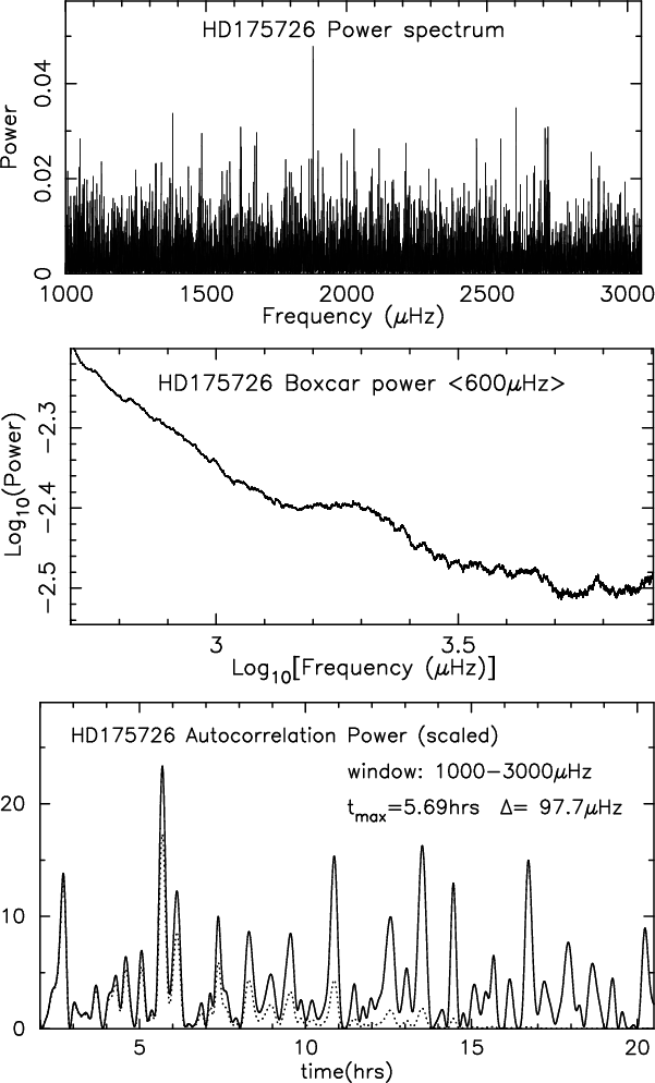 |
Figure 5:
a) Power spectra for HD 175726: b) result of applying a boxcar of |
| Open with DEXTER | |
The autocorrelation power, filtered by a ![]() window between
window between
![]() Hz, is shown in Fig. 5c. The highest peak away from zero is at t=5.69 h, which, if due to the large separations, gives a mean large separation
Hz, is shown in Fig. 5c. The highest peak away from zero is at t=5.69 h, which, if due to the large separations, gives a mean large separation
![]() Hz. Also shown in Fig. 5c as the dotted line is the autocorrelation power obtained using a boxcar power spectrum with averaging over
Hz. Also shown in Fig. 5c as the dotted line is the autocorrelation power obtained using a boxcar power spectrum with averaging over ![]() Hz. It should be stressed that one is here fighting to extract a signal from the noise and the results will differ somewhat depending on how one treats the data: filtering out low frequency variations, filling gaps by linear interpolation with or without added noise, and suppressing or not harmonics of the orbital period. Nevertheless the general behaviour is found with different procedures (see Mosser et al. 2009, for a more detailed discussion on the statistical robustness of the results).
Hz. It should be stressed that one is here fighting to extract a signal from the noise and the results will differ somewhat depending on how one treats the data: filtering out low frequency variations, filling gaps by linear interpolation with or without added noise, and suppressing or not harmonics of the orbital period. Nevertheless the general behaviour is found with different procedures (see Mosser et al. 2009, for a more detailed discussion on the statistical robustness of the results).
 |
Figure 6:
Variation of Large separation with frequency for HD 175726 for a set of narrow window of |
| Open with DEXTER | |
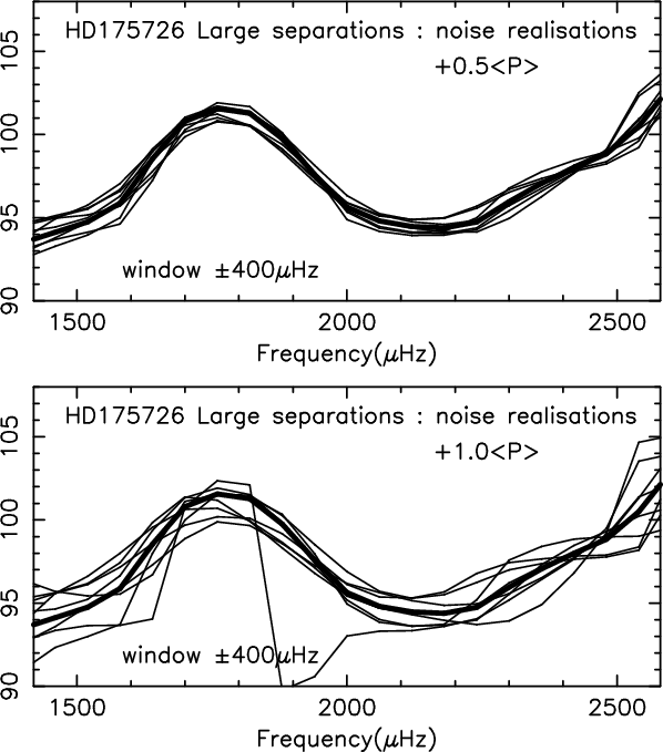 |
Figure 7:
Autocorrelation power for HD 175726 |
| Open with DEXTER | |
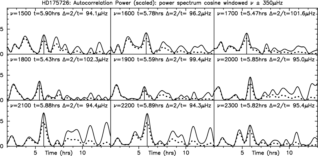 |
Figure 8:
Autocorrelation power for HD 175726 |
| Open with DEXTER | |
I then added exponentially distributed noise to the power spectrum with a mean of 0.5 and 1.0 times the average power
![]() in the frequency range
in the frequency range
![]() Hz, and repeated the calculations for a
Hz, and repeated the calculations for a ![]() 400
400 ![]() Hz window; the results are shown in Figs. 7a and b, the thick line being the result with no added noise. These results suggest that the signal is there, but this does not of course prove that the signal is due to the variation
Hz window; the results are shown in Figs. 7a and b, the thick line being the result with no added noise. These results suggest that the signal is there, but this does not of course prove that the signal is due to the variation
![]() .
Estimates of the error on the autocorrelation due to time resolution, window width, and interference between signal and noise are considered in Mosser et al. (2009). They also test the reliability of the shape displayed in Fig. 6 with an H0 test and concluded that the hypothesis that the signal is real is only rejected at the
.
Estimates of the error on the autocorrelation due to time resolution, window width, and interference between signal and noise are considered in Mosser et al. (2009). They also test the reliability of the shape displayed in Fig. 6 with an H0 test and concluded that the hypothesis that the signal is real is only rejected at the ![]()
![]() level.
level.
As mentioned above, one is here fighting against the noise - just how much is illustrated in Fig. 8, which gives the autocorrelation power for a window of half width ![]() Hz centred on frequencies in the range 1500 and
Hz centred on frequencies in the range 1500 and ![]() Hz. A peak around
Hz. A peak around ![]() Hz can just be seen, although how significant it is needs to be the subject of further investigation. The dotted line in Fig. 8 is the autocorrelation power using a boxcar spectrum averaging over
Hz can just be seen, although how significant it is needs to be the subject of further investigation. The dotted line in Fig. 8 is the autocorrelation power using a boxcar spectrum averaging over ![]() Hz.
Hz.
4 Analysis and modelling
I first take the simplest possible model where the peaks in the frequency power spectrum are given by delta functions so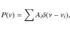 |
(4) |
where
As shown by Roxburgh and Vorontsov (2000), by matching the inner and outer solutions of the equations governing the oscillations at an intermediate radius rf, the eigenfrequencies
![]() satisfy the eigenfrequency equation
satisfy the eigenfrequency equation
 |
(5) |
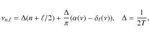
where
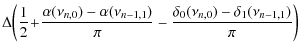
![\begin{displaymath}\Delta_{n,\ell}=\Delta\left(1 + {1\over\pi}\big[ \alpha(\nu_{...
..._\ell(\nu_{n.\ell}) + \delta_\ell(\nu_{n-1,\ell})\big]\right).
\end{displaymath}](/articles/aa/full_html/2009/40/aa11906-09/img99.png) |
(6) |
Consider first the simple model consisting solely of a pair of adjacent modes
| F(t) | = | ![$\displaystyle \int_0^\infty \left[a_0 \delta(\nu-\nu_{0})
+ a_1 \delta(\nu-\nu_{1})\right] {\rm e}^{2\pi {\rm i}\nu t }$](/articles/aa/full_html/2009/40/aa11906-09/img102.png) |
(7) |
| = |
where the ai are the amplitudes of the modes in the power spectrum.
The autocorrelation power (the power spectrum of the power spectrum) is |F|2 which is then
![\begin{displaymath}A^2 = a_0^2 + a_1^2 + 2 a_0~a_1 \cos[ 2\pi (\nu_1-\nu_0) t].
\end{displaymath}](/articles/aa/full_html/2009/40/aa11906-09/img104.png) |
(8) |
This has its first peak (beyond zero) when
However if, as is the real case,
![]() vary with frequency and
vary with frequency and
![]() ,
the above pair analysis remains valid but
,
the above pair analysis remains valid but
![]() .
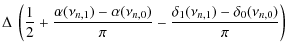
I therefore define the half large separations
.
I therefore define the half large separations
| (9) |
Their sum gives the ordinary large separations
| (10) |
and difference the small separations (Roxburgh 1993, 2009)
| (11) |
The power from the pair of modes
![]() is
is
![\begin{displaymath}A^2 = \left( a_0^2 + a_1^2 + 2 a_0~a_1 \cos[ 2\pi\Delta_{10}(n) t] \right ),
\end{displaymath}](/articles/aa/full_html/2009/40/aa11906-09/img115.png) |
(12) |
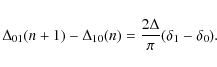
which has its first maximum at
![\begin{displaymath}A^2 = \left( a_0^2 + a_1^2 + 2 a_0~a_1 \cos[ 2\pi\Delta_{01}(n+1) t] \right ),
\end{displaymath}](/articles/aa/full_html/2009/40/aa11906-09/img118.png) |
(13) |
and has its first maximum at
As can be seen from Eq. (5)
| |
= |  |
(14) |
| = |  |
(15) |
so even if
 |
(16) |
For the Sun the difference
For a large set of eigenfrequencies within a window (including ![]() )
the situation is more complicated since one cannot just add up the power in each pair but have to take the full Fourier transform. However one can see that if there is only one pair
)
the situation is more complicated since one cannot just add up the power in each pair but have to take the full Fourier transform. However one can see that if there is only one pair
![]() in a window, the position of the first maximum will be different from that with just the
overlapping pair
in a window, the position of the first maximum will be different from that with just the
overlapping pair
![]() .
If there are a number of such sets within a window then one may expect the
first peak in the autocorrelation power spectrum to be determined by the full large separations
.
If there are a number of such sets within a window then one may expect the
first peak in the autocorrelation power spectrum to be determined by the full large separations
![]() .
Note that, at least for the Sun, the difference between
.
Note that, at least for the Sun, the difference between ![]() and
and ![]() is much smaller that that between
is much smaller that that between
![]() and
and
![]() since the inner phase shifts
since the inner phase shifts
![]() differ by much more than the change in
differ by much more than the change in
![]() ,
and
,
and ![]() between adjacent frequencies.
Of course the actual windowed autocorrelation for a small set of frequencies depends on the amplitudes of all significant modes
(
between adjacent frequencies.
Of course the actual windowed autocorrelation for a small set of frequencies depends on the amplitudes of all significant modes
(
![]() )
within the window and on noise peaks. For a theoretical model this could be calculated but for a real data set one can do no more than predict that for very narrow windows the first peak of the autocorrelation function will vary depending on whether it is an
)
within the window and on noise peaks. For a theoretical model this could be calculated but for a real data set one can do no more than predict that for very narrow windows the first peak of the autocorrelation function will vary depending on whether it is an ![]() pair or an
pair or an ![]() pair at the centre of the window, but for a wider window the peak is determined by a locally averaged large separation.
This is the origin of the oscillatory behaviour of the
pair at the centre of the window, but for a wider window the peak is determined by a locally averaged large separation.
This is the origin of the oscillatory behaviour of the ![]()
![]() Hz windowed results for HD 49933 displayed in
Fig. 4c. It offers the possibility of determining the inner phase shift difference
Hz windowed results for HD 49933 displayed in
Fig. 4c. It offers the possibility of determining the inner phase shift difference
![]() as a function of frequency, which is an important diagnostic of the stellar interior and convective boundaries (Roxburgh 2009).
as a function of frequency, which is an important diagnostic of the stellar interior and convective boundaries (Roxburgh 2009).
To demonstrate that this technique can, in principle, work I constructed a theoretician's ideal artificial noise free power spectrum by prescribing a surface phase shift
![]() and inner phase shits
and inner phase shits
![]() ,
with the eigenfrequencies determined by the Eigenfrequency equation (Roxburgh & Vorontsov 2000)
,
with the eigenfrequencies determined by the Eigenfrequency equation (Roxburgh & Vorontsov 2000)
| (17) |
To produce a model with similar characteristics to HD 175726 the model had an acoustic radius of T=5000 s, and
| |
= | ![$\displaystyle {4.5\over 0.5 +\nu_{2}}
\left(1+{0.03375 \over \nu_{2}^2}
\sin\left[{2\pi\nu/\nu_0} +1.5\right] \right)$](/articles/aa/full_html/2009/40/aa11906-09/img142.png) |
(18) |
| = | (19) |
where
The individual line profiles were taken to be Lorentzians of width ![]() Hz and the amplitude ratios for modes with
Hz and the amplitude ratios for modes with
![]() in the ratios
1, 1.334, 0.35, 0.016. The resulting powers spectrum was then scaled by the factor
in the ratios
1, 1.334, 0.35, 0.016. The resulting powers spectrum was then scaled by the factor
![]() with
with
![]() The resulting model power spectrum is shown in Fig. 9a.
Applying the narrow windowed autocorrelation analysis with windows of
The resulting model power spectrum is shown in Fig. 9a.
Applying the narrow windowed autocorrelation analysis with windows of ![]()
![]() Hz yielded the curves displayed in Fig. 9b, together with the values of
Hz yielded the curves displayed in Fig. 9b, together with the values of ![]() derived from the frequencies of the model. As expected the wider windows depart further from the actual large separations since the wider the window the greater the smoothing of the actual separations. The narrowest window shows the beginnings of a periodic modulation due to the difference between the half large separations
derived from the frequencies of the model. As expected the wider windows depart further from the actual large separations since the wider the window the greater the smoothing of the actual separations. The narrowest window shows the beginnings of a periodic modulation due to the difference between the half large separations
![]() and
and
![]() .
.
I then added exponential noise to this artificial power spectrum as shown in Fig. 10a, which is on the same scale as Fig. 9a. The noiseless power spectrum is shown in white in this figure. The variation of the large separations with frequency as determined from frequency windowed autocorrelation with windows of ![]()
![]() Hz are shown in Fig. 10b.
Hz are shown in Fig. 10b.
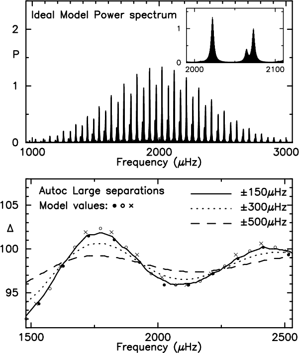 |
Figure 9:
a) Ideal model power spectrum; the inset shows an example of the line profiles. b) Large separation
|
| Open with DEXTER | |
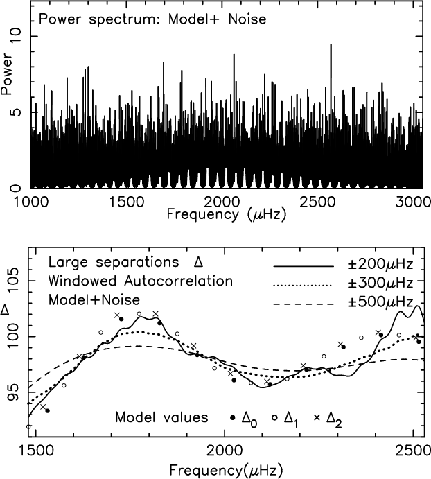 |
Figure 10:
a) Ideal model power spectrum + added noise; the noiseless power spectrum is shown in white. b) Large separation
|
| Open with DEXTER | |
Comparison of these results with those for HD 175726 shown in Fig. 6 suggests one can extract some information on the large scale variations of
![]() by this procedure.
by this procedure.
Returning to the noiseless model power spectrum I then took very narrow frequency windows of ![]()
![]() Hz to test whether this can give the half large separations
Hz to test whether this can give the half large separations
![]() defined above in Eq. (9). Figure 11a shows the results for the full model power spectrum. The autocorrelation values show the same general behaviour as the exact values of the frequencies but somewhat offset. That this is due to the contribution of the
defined above in Eq. (9). Figure 11a shows the results for the full model power spectrum. The autocorrelation values show the same general behaviour as the exact values of the frequencies but somewhat offset. That this is due to the contribution of the ![]() modes is clear from Fig. 11b where the model power spectrum was taken to only have
modes is clear from Fig. 11b where the model power spectrum was taken to only have ![]() modes; in this case the half large separations are faithfully reproduced.
modes; in this case the half large separations are faithfully reproduced.
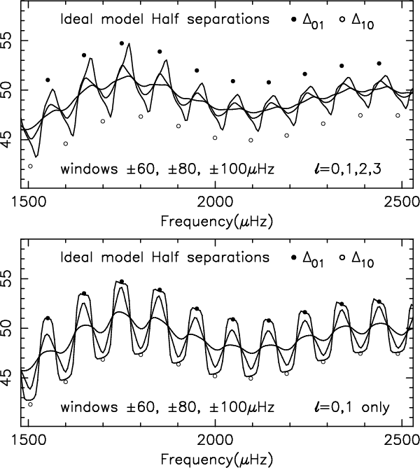 |
Figure 11:
a) Half large separation
|
| Open with DEXTER | |
5 HD 181420
HD 181420 is an F2 (mv=6.57) star observed by CoRoT in a 156 day run (Michel et al. 2008, Barban et al. 2009). Details of the data reduction are given in Barban et al. (2009), but are essentially the same as described above for HD 49933. The power spectrum is given in Fig. 12a and a boxcar spectrum in Fig. 12b. There is excess power in the p-mode frequency range
![]() Hz. Details of the extraction of frequencies are given in Barban et al. (2009) but as with HD 49933 it is difficult to discriminate between peaks corresponding to modes
Hz. Details of the extraction of frequencies are given in Barban et al. (2009) but as with HD 49933 it is difficult to discriminate between peaks corresponding to modes ![]() and those corresponding to
and those corresponding to ![]() ;
Barban et al. (2009) give frequency sets for both (Scenarios 1 and 2). I here give the results of applying narrow frequency windowed autocorrelations to the time series and see if one can differentiate between them.
;
Barban et al. (2009) give frequency sets for both (Scenarios 1 and 2). I here give the results of applying narrow frequency windowed autocorrelations to the time series and see if one can differentiate between them.
Figure 13a shows the autocorrelation power in a wide (![]() Hz) window with a clean peak at
Hz) window with a clean peak at
![]() hrs corresponding to a mean large separation of
hrs corresponding to a mean large separation of ![]() Hz, and a secondary peak at
Hz, and a secondary peak at
![]() .
The rapid decrease in amplitude between the two peaks is again indicative of the large line widths in the power spectrum. Figure 13b shows the results of using a narrower frequency window of full width
.
The rapid decrease in amplitude between the two peaks is again indicative of the large line widths in the power spectrum. Figure 13b shows the results of using a narrower frequency window of full width ![]() Hz. Again there is variation of
Hz. Again there is variation of ![]() with frequency.
with frequency.
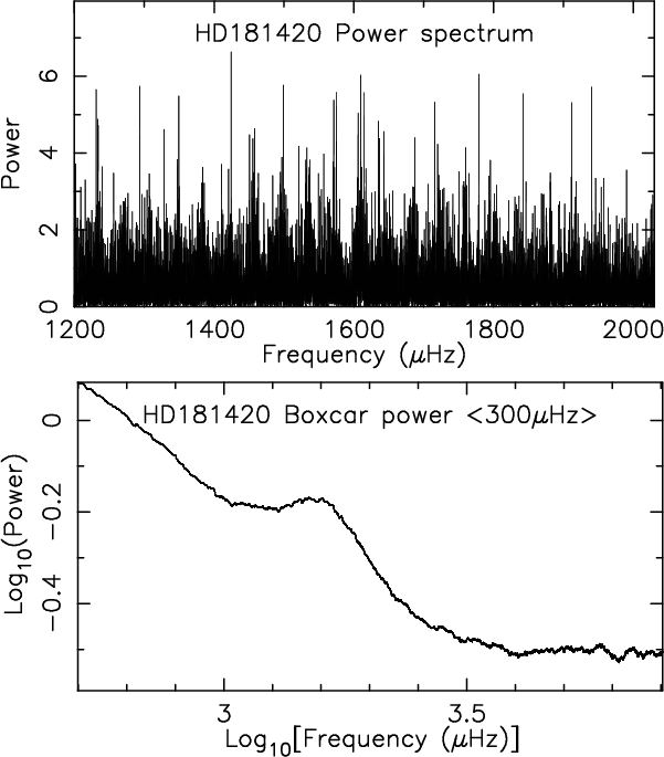 |
Figure 12:
a) HD 181420 Power spectrum. b) Boxcar power spectrum full width |
| Open with DEXTER | |
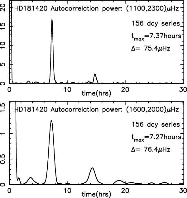 |
Figure 13:
a) Autocorrelation power for HD 181420 with |
| Open with DEXTER | |
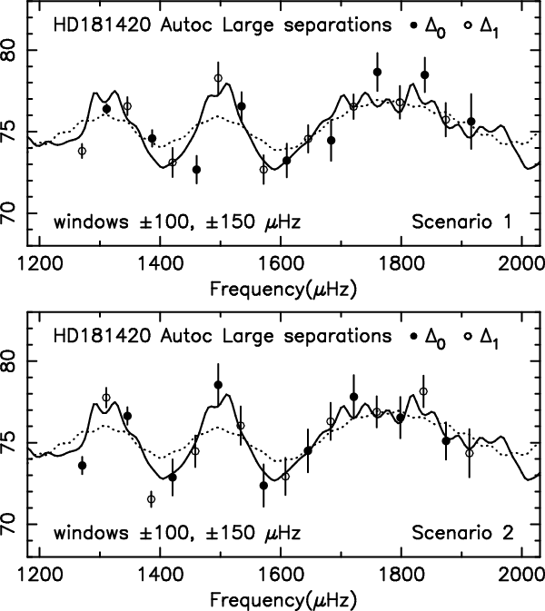 |
Figure 14:
Autocorrelation Large separations for HD 181420 with |
| Open with DEXTER | |
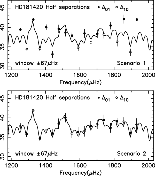 |
Figure 15:
Autocorrelation Half Large separations for HD 181420 with |
| Open with DEXTER | |
I then used narrow windows of ![]()
![]() Hz and determined the local large separations
Hz and determined the local large separations
![]() ,
the results are in Fig. 14a for Barban's Scenario 1, and in Fig. 14b for Scenario 2. The points and error bars are from the frequency sets given in Barban et al. There is not much to choose between the fit of the
,
the results are in Fig. 14a for Barban's Scenario 1, and in Fig. 14b for Scenario 2. The points and error bars are from the frequency sets given in Barban et al. There is not much to choose between the fit of the ![]()
![]() Hz windowed results to the separations determined from the frequencies - possibly Scenario 2 is a little better than Scenario 1.
Hz windowed results to the separations determined from the frequencies - possibly Scenario 2 is a little better than Scenario 1.
Since the values of ![]() vary substantially with frequency a better test would be to use even narrower windows which give the half large separations
vary substantially with frequency a better test would be to use even narrower windows which give the half large separations
![]() as in Fig. 11. The results for a window of
as in Fig. 11. The results for a window of ![]()
![]() Hz are shown in Fig. 15 for both scenarios. Here Scenario 2 gives a better fit than Scenario 1, suggesting that Scenario 2 is the correct identification of the modes.
Hz are shown in Fig. 15 for both scenarios. Here Scenario 2 gives a better fit than Scenario 1, suggesting that Scenario 2 is the correct identification of the modes.
6 HD 181906
HD 181906 is an F8 (mv=7.65) star observed by CoRoT for 156 days, that displays very low p-mode power in the frequency range
![]() Hz (Michel et al. 2008, García et al. 2009); it is considerably fainter than HD 49933 and HD 181420. Figure 16a gives the power spectrum and Fig. 16b the boxcar spectrum which shows an excess of power in the p-mode frequency range
Hz (Michel et al. 2008, García et al. 2009); it is considerably fainter than HD 49933 and HD 181420. Figure 16a gives the power spectrum and Fig. 16b the boxcar spectrum which shows an excess of power in the p-mode frequency range
![]() Hz. The power spectrum was derived from the time series by the same procedures as for HD 49933. Figure 16c gives the autocorrelation power for a wide frequency window of
Hz. The power spectrum was derived from the time series by the same procedures as for HD 49933. Figure 16c gives the autocorrelation power for a wide frequency window of ![]() Hz. There is a clear peak at
Hz. There is a clear peak at
![]() hrs corresponding to a mean large separation of
hrs corresponding to a mean large separation of ![]() Hz and a small second peak at
Hz and a small second peak at
![]() .
.
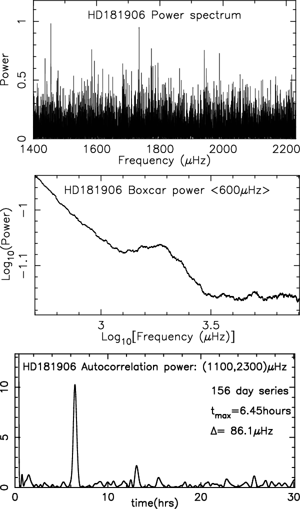 |
Figure 16:
a) Power spectrum of HD 181906. b) Boxcar power spectrum with |
| Open with DEXTER | |
Extracting frequencies from the power spectrum is difficult as the signal to noise is small and rotational splitting, line widths and (![]() )
separations all overlap. By making severe constraints on the fitting procedure (mode widths and mode heights set equal over the fitted frequency range) values of nine
)
separations all overlap. By making severe constraints on the fitting procedure (mode widths and mode heights set equal over the fitted frequency range) values of nine
![]() frequencies were obtained by García et al. (2009). These differ from those obtained for a smaller frequency sets (5 n values) obtained by Verner (private communication) with less rigid constraints on the fitting procedure, and are only marginally consistent within the larger formal errors of Verner's analysis. Again there is uncertainty over which peaks correspond to
frequencies were obtained by García et al. (2009). These differ from those obtained for a smaller frequency sets (5 n values) obtained by Verner (private communication) with less rigid constraints on the fitting procedure, and are only marginally consistent within the larger formal errors of Verner's analysis. Again there is uncertainty over which peaks correspond to ![]() and which to rotationally split
and which to rotationally split ![]() modes; these two alternatives are labelled Scenario A and B in García et al.
modes; these two alternatives are labelled Scenario A and B in García et al.
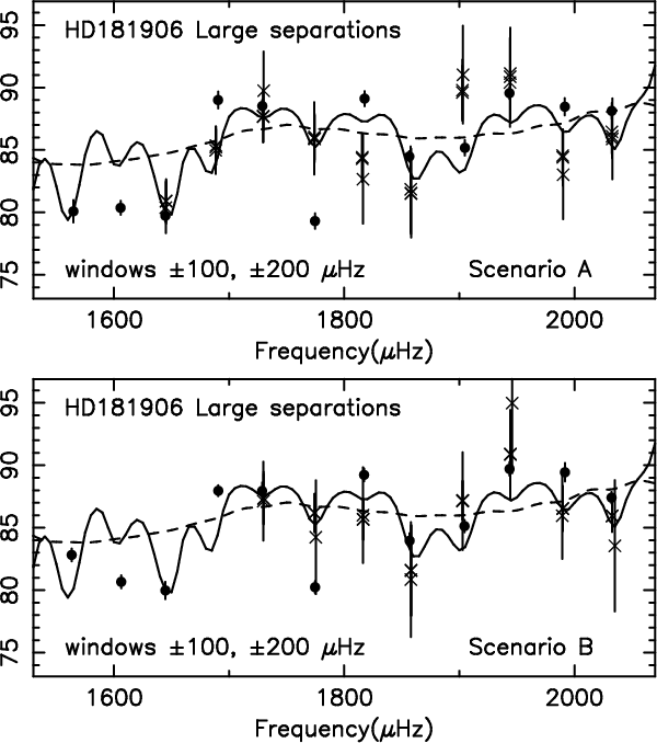 |
Figure 17:
a) Autocorrelation Large separations for HD 181906 with |
| Open with DEXTER | |
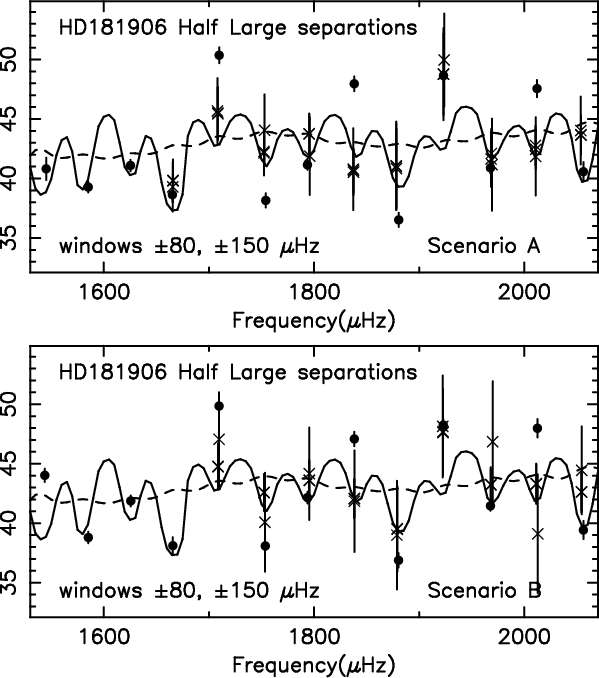 |
Figure 18:
a) Autocorrelation Half Large separations for HD 181906 with |
| Open with DEXTER | |
I then used narrow windows of
![]() Hz and determined the local large separations
Hz and determined the local large separations
![]() from the peaks in the autocorrelation power; the results are in Fig. 17a for García's Scenario A and Fig. 17b for Scenario B. The circles in these diagrams are the values obtained with García's frequencies and the crosses those from 3 different analyses by Verner, each with their estimated formal errors. The considerable difference between values from different frequency extraction algorithms illustrates the difficulty in deriving reliable values of the frequencies for this star Figs. 18 gives the values of the half large separations using an
from the peaks in the autocorrelation power; the results are in Fig. 17a for García's Scenario A and Fig. 17b for Scenario B. The circles in these diagrams are the values obtained with García's frequencies and the crosses those from 3 different analyses by Verner, each with their estimated formal errors. The considerable difference between values from different frequency extraction algorithms illustrates the difficulty in deriving reliable values of the frequencies for this star Figs. 18 gives the values of the half large separations using an ![]()
![]() Hz window for the two Scenarios. The agreement between the autocorrelation values and those from any frequency set is not good. Further work needs to be done on both frequency extraction and the windowed autocorrelations to see if one can obtain agreement similar to that for HD 181420 in Fig. 15b.
Hz window for the two Scenarios. The agreement between the autocorrelation values and those from any frequency set is not good. Further work needs to be done on both frequency extraction and the windowed autocorrelations to see if one can obtain agreement similar to that for HD 181420 in Fig. 15b.
7 Conclusions
The principal goal of this paper was to show that narrow frequency windowed autocorrelation can, in principle, reveal information on the variation of the large separation with frequency and therefore constitutes a tool that might be useful in obtaining some information about a star even when individual frequencies cannot be extracted, or modes cannot be identified. Much remains to be done to refine the technique: the theoretical analysis needs to be further developed and the nature of the interaction of noise with the autocorrelation power better understood.
However the analysis presented here suggests that narrow frequency windowed autocorrelations can yield the variation with frequency of the large separations
![]() and that very narrow windows can yield the half large separations
and that very narrow windows can yield the half large separations
![]() and
and
![]() and thereby help to resolve the uncertainty over mode recognition between
and thereby help to resolve the uncertainty over mode recognition between ![]() and
and ![]() modes.
modes.
Since the difference between the half large separations is determined by the inner phase shift difference
![]() ,
this gives a diagnostic of the internal structure of a star (Roxburgh 2009). This will be explored in a subsequent communication.
,
this gives a diagnostic of the internal structure of a star (Roxburgh 2009). This will be explored in a subsequent communication.
Acknowledgements
I thank the UK Science and Technology Facilities Council (STFC) which supported this work under grants PPA/G/S/2003/00137 and PP/E001793/1 and Graham Verner for the determination of the unpublished frequencies used in this paper.
References
- Appourchaux, T., Michel, E., Auvergne, M., et al. 2008, A&A, 488, 705 [NASA ADS] [CrossRef] [EDP Sciences] (In the text)
- Barban, C., Deheuvels, S., Baudin, F., et al. 2009, A&A, 506, 51 [CrossRef] [EDP Sciences] (In the text)
- Brodskii, M. A., & Vorontsov, S. V. 1989, Astron. Zh., 15, 61 (English version: Sov. Ast. Lett. 1989. 15, 27) (In the text)
- Gabriel, M., Grec, G., Renaud, C., et al. 1998, A&A, 338, 1109 [NASA ADS]
- García, R., Régulo, C., Samadi, R., et al. 2009, A&A, 506, 41 [CrossRef] [EDP Sciences] (In the text)
- Kallinger, T., Gruberbauer, M., Guenther, D. B., Fossati, L., & Weiss, W. W. 2008, A&A, submitted [arXiv:0811.4686v1] (In the text)
- Kholikov S., & Hill, F. 2008, Sol. Phys., 251, 157 [NASA ADS] [CrossRef] (In the text)
- Michel, E., Baglin, A. Auvergne, M., et al. 2008, Science, 322, 558 [NASA ADS] [CrossRef] (In the text)
- Mosser, B., Michel, E., Appourchaux, T., et al. 2009, A&A, 506, 33 [CrossRef] [EDP Sciences] (In the text)
- Press, W. H., Flannery, B. P., Teukolsky A. S., & Vetterling, W. T. 1992, Numerical Recipes (CUP), 383 (In the text)
- Roxburgh, I. W. 1993, in PRISMA, Report of Phase A Study, ed. T. Appourchaux, T., ESA SCI(93), 31 (In the text)
- Roxburgh, I. W. 2009, A&A, 493, 185 [NASA ADS] [CrossRef] [EDP Sciences] (In the text)
- Roxburgh, I. W., & Vorontsov, S. V. 1994, MNRAS, 267, 297 [NASA ADS] (In the text)
- Roxburgh, I. W., & Vorontsov, S. V. 2000, MNRAS, 317, 141 [NASA ADS] [CrossRef] (In the text)
- Roxburgh, I. W., & Vorontsov, S. V. 2006a, MNRAS, 369, 1491 [NASA ADS] [CrossRef] (In the text)
- Roxburgh, I. W., & Vorontsov, S. V. 2006b, MNRAS, 379, 801 [NASA ADS] [CrossRef]
- Samadi, R., Fialho, F., Costa, J. E. S., et al. 2006, ESA SP 1306, 317, corrected in [arXiv:astro-ph/0703354] (In the text)
- Vorontsov, S. V., & Zharkov, V. N. 1988, Itogi Nauki Tek, Ser Astro, 38, 253 (English version: Astro & Space Phys Rev. 1989, 7, 1) (In the text)
- Vorontsov, S. V., & Zharkov, V. N. 1989, Astro & Space Phys. Rev., 7, 1 [NASA ADS]
Footnotes
- ... CoRoT
![[*]](/icons/foot_motif.png)
- The CoRoT space mission, launched on 2006 December 27, was developed and is operated by CNES, with the participation of the Science Programmes of ESA, ESA's RSSD, Austria, Belgium, Brazil, Germany and Spain.
All Figures
| |
Figure 1:
HD 49933 autocorrelation, frequency windowed between
|
| Open with DEXTER | |
| In the text | |
| |
Figure 2: HD 49933 power spectrum. |
| Open with DEXTER | |
| In the text | |
| |
Figure 3:
Frequency windowed autocorrelation power for HD 49933 (scaled): a) windowed between
|
| Open with DEXTER | |
| In the text | |
| |
Figure 4:
a) Variation of large separation with frequency for HD 49933 from autocorrelation with a |
| Open with DEXTER | |
| In the text | |
| |
Figure 5:
a) Power spectra for HD 175726: b) result of applying a boxcar of |
| Open with DEXTER | |
| In the text | |
| |
Figure 6:
Variation of Large separation with frequency for HD 175726 for a set of narrow window of |
| Open with DEXTER | |
| In the text | |
| |
Figure 7:
Autocorrelation power for HD 175726 |
| Open with DEXTER | |
| In the text | |
| |
Figure 8:
Autocorrelation power for HD 175726 |
| Open with DEXTER | |
| In the text | |
| |
Figure 9:
a) Ideal model power spectrum; the inset shows an example of the line profiles. b) Large separation
|
| Open with DEXTER | |
| In the text | |
| |
Figure 10:
a) Ideal model power spectrum + added noise; the noiseless power spectrum is shown in white. b) Large separation
|
| Open with DEXTER | |
| In the text | |
| |
Figure 11:
a) Half large separation
|
| Open with DEXTER | |
| In the text | |
| |
Figure 12:
a) HD 181420 Power spectrum. b) Boxcar power spectrum full width |
| Open with DEXTER | |
| In the text | |
| |
Figure 13:
a) Autocorrelation power for HD 181420 with |
| Open with DEXTER | |
| In the text | |
| |
Figure 14:
Autocorrelation Large separations for HD 181420 with |
| Open with DEXTER | |
| In the text | |
| |
Figure 15:
Autocorrelation Half Large separations for HD 181420 with |
| Open with DEXTER | |
| In the text | |
| |
Figure 16:
a) Power spectrum of HD 181906. b) Boxcar power spectrum with |
| Open with DEXTER | |
| In the text | |
| |
Figure 17:
a) Autocorrelation Large separations for HD 181906 with |
| Open with DEXTER | |
| In the text | |
| |
Figure 18:
a) Autocorrelation Half Large separations for HD 181906 with |
| Open with DEXTER | |
| In the text | |
Copyright ESO 2009
Current usage metrics show cumulative count of Article Views (full-text article views including HTML views, PDF and ePub downloads, according to the available data) and Abstracts Views on Vision4Press platform.
Data correspond to usage on the plateform after 2015. The current usage metrics is available 48-96 hours after online publication and is updated daily on week days.
Initial download of the metrics may take a while.