| Issue |
A&A
Volume 505, Number 3, October III 2009
|
|
|---|---|---|
| Page(s) | 955 - 968 | |
| Section | Astrophysical processes | |
| DOI | https://doi.org/10.1051/0004-6361/200912653 | |
| Published online | 18 August 2009 | |
Reynolds stresses from hydrodynamic turbulence with shear and rotation![[*]](/icons/foot_motif.png)
J. E. Snellman1 - P. J. Käpylä1,2 - M. J. Korpi1 - A. J. Liljeström1
1 - Observatory, PO Box 14, 00014 University of Helsinki,
Finland
2 - NORDITA, Roslagstullsbacken 23, 10691 Stockholm, Sweden
Received 8 June 2009 / Accepted 3 August 2009
Abstract
Aims. We study the Reynolds stresses which describe turbulent momentum transport from turbulence affected by large-scale shear and rotation.
Methods. Three-dimensional numerical simulations are used to study turbulent transport under the influences of large-scale shear and rotation in homogeneous, isotropically forced turbulence. We study three cases: one with only shear, and two others where in addition to shear, rotation is present. These cases differ by the angle (0 or
![]() )
the rotation vector makes with respect to the z-direction. Two subsets of runs are performed with both values of
)
the rotation vector makes with respect to the z-direction. Two subsets of runs are performed with both values of ![]() where either rotation or shear is kept constant. When only shear is present, the off-diagonal stress can be described by turbulent viscosity whereas if the system also rotates, nondiffusive contributions (
where either rotation or shear is kept constant. When only shear is present, the off-diagonal stress can be described by turbulent viscosity whereas if the system also rotates, nondiffusive contributions (![]() -effect) to the stress can arise. Comparison of the direct simulations are made with analytical results from a simple closure model.
-effect) to the stress can arise. Comparison of the direct simulations are made with analytical results from a simple closure model.
Results. We find that the turbulent viscosity is of the order of the first order smoothing result in the parameter regime studied and that for sufficiently large Reynolds numbers the Strouhal number, describing the ratio of correlation to turnover times, is roughly 1.5. This is consistent with the closure model based on the minimal tau-approximation which produces a reasonable fit to the simulation data for similar Strouhal numbers. In the cases where rotation is present, separating the diffusive and nondiffusive components of the stress turns out to be challenging but taking the results at face value, we can obtain nondiffusive contributions of the order of 0.1 times the turbulent viscosity. We also find that the simple closure model is able to reproduce most of the qualitative features of the numerical results provided that the Strouhal number is of the order of unity.
Key words: hydrodynamics - turbulence - accretion, accretion disks - Sun: rotation - stars: rotation
1 Introduction
Turbulent angular momentum transport is considered to be of importance in various astrophysical objects, such as accretion disks (e.g. Balbus & Hawley 1998) and convectively unstable layers within stars (e.g. Rüdiger 1989) where they take part in shaping the internal rotation profile of the object. Due to the immense numerical requirements, direct global simulations of these systems are not yet feasible in large quantities, although some simulations are able to capture many features of, for example, the solar rotation profile (see e.g. Robinson & Chan 2001; Brun & Toomre 2002; Miesch et al. 2006,2008). However, in many cases it would be desirable to be able to use simplified, and computationally less demanding, mean-field models where the effects of small-scale turbulence are accurately parameterized in some collective way. Although a rich literature of mean-field models of solar internal rotation exist (e.g. Brandenburg et al. 1992; Küker et al. 1993; Kitchatinov & Rüdiger 2005; Rempel 2005), many of the models use simple and often untested parameterizations of the turbulent quantities.
Parameterizing turbulence entails a closure model for the
turbulent correlations. One of the most often used closures in
astrophysics is the ![]() -prescription (Shakura & Sunyaev
1973), widely used in accretion disk theory, which
relates the turbulent viscosity to the local gas pressure. This very
simple parameterization allows analytically tractable solutions of
accretion disk structure but suffers from the drawback that important
physics, such as magnetic fields, are not taken into account.
More recently, dynamical turbulent closure models
yielding all the relevant components of the Reynolds and Maxwell
stresses in simplified setups with homogeneous magnetized shear flows
have started to appear (e.g. Ogilvie 2003; Pessah et al. 2006).
-prescription (Shakura & Sunyaev
1973), widely used in accretion disk theory, which
relates the turbulent viscosity to the local gas pressure. This very
simple parameterization allows analytically tractable solutions of
accretion disk structure but suffers from the drawback that important
physics, such as magnetic fields, are not taken into account.
More recently, dynamical turbulent closure models
yielding all the relevant components of the Reynolds and Maxwell
stresses in simplified setups with homogeneous magnetized shear flows
have started to appear (e.g. Ogilvie 2003; Pessah et al. 2006).
For these more sophisticated models to be useful, they need to be validated somehow. The obvious validation method is to compare to numerical simulations that work in a parameter regime which is as similar as possible. Comparisons of closure models with numerical simulations of the magnetorotational instability in periodic local slab geometry have appeared recently (e.g. Pessah et al. 2008; Liljeström et al. 2009) and yield encouraging results in that the closure models are able to capture, at least qualitatively, many of the main features of the numerical simulations. However, these studies concentrate on a situation where the turbulence is generated via the magnetorotational instability (Velikhov 1959; Chandrasekhar 1961; Balbus & Hawley 1991), the nonlinear behaviour of which is still not very well understood (e.g. Fromang et al. 2007).
In the present paper we avoid these complications and consider only the simplest possible hydrodynamic case and assume that isotropic and homogeneous background turbulence already exists in the system upon which large-scale shear and rotation can be imposed. Such turbulence can be generated by using suitable forcing in the Navier-Stokes equation. Although flows of this kind are not likely to occur in nature, they are perfect testbeds for the developement and testing of turbulent closure models.
The present paper is a continuation to an earlier study (Käpylä &
Brandenburg 2008, hereafter KB08; see also Käpylä &
Brandenburg 2007) where simulations of anisotropic homogeneous
turbulence under the influence of rotation were compared to a simple
closure model applying the so-called tau-approximation (hereafter MTA,
see e.g. Blackman
& Field 2002,2003; Brandenburg et al. 2004). In the
present study we adopt an isotropic forcing and add a large-scale
shear flow using the shearing box approximation. Such a setup
allows us to determine the turbulent
viscosity (see preliminary results in Käpylä & Brandenburg
2007; and Käpylä et al. 2009). The imposed shear
flow also introduces anisotropy into the turbulence which, under the
influence of rotation, can produce additional non-diffusive Reynolds
stresses (Leprovost & Kim 2007,2008a,b), which are more
commonly known as the ![]() -effect (Krause & Rüdiger
1974; Rüdiger 1980, 1989). We make an effort to
separate the diffusive and nondiffusive contributions from the
numerical data. As in KB08, one of the main goals of the study is to
compare the simulation results to a simple closure model, similar to
that introduced by Ogilvie (2003).
-effect (Krause & Rüdiger
1974; Rüdiger 1980, 1989). We make an effort to
separate the diffusive and nondiffusive contributions from the
numerical data. As in KB08, one of the main goals of the study is to
compare the simulation results to a simple closure model, similar to
that introduced by Ogilvie (2003).
The remainder of the paper is organised as follows: the models used in the study are presented in Sect. 2, whereas Sects. 3 and 4 give the results and conclusions of the study, respectively.
2 The model and methods
2.1 Basic equations
We model compressible hydrodynamic turbulence in shearing periodic
cube of size ![]() .
The gas obeys an isothermal equation of state
characterized by a constant speed of sound,
.
The gas obeys an isothermal equation of state
characterized by a constant speed of sound, ![]() .
The
continuity and Navier-Stokes equations read
.
The
continuity and Navier-Stokes equations read
 |
(1) |
where
 |
(3) |
where
 |
(4) |
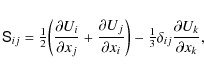
is the traceless rate of strain tensor. The forcing function
| (5) |
where
 |
(6) |
where
The numerical simulations were performed with the
P ENCIL C ODE![]() ,
which uses sixth-order accurate finite differences in space, and a
third-order accurate time-stepping scheme (Brandenburg & Dobler
2002; Brandenburg
2003). Resolutions up to 10243 grid points were
used.
,
which uses sixth-order accurate finite differences in space, and a
third-order accurate time-stepping scheme (Brandenburg & Dobler
2002; Brandenburg
2003). Resolutions up to 10243 grid points were
used.
2.2 Dimensionless units and parameters
We obtain nondimensional variables by setting
| (7) |
This means that the units of length, time, and density are
| (8) |
However, in what follows we present the results in explicitly dimensionless form using the quantities above.
The strengths of shear, rotation, and viscous effects are measured by the
shear, Coriolis and Reynolds numbers, respectively, based on the
forcing scale as
See Fig. 1 for a typical snapshot from a high resolution run with
2.3 Coordinate system, averaging, and error estimates
The simulated domain can be thought to represent a small rectangular portion of a spherical body of gas. We choose (x,y,z) to correspond to
where
Firstly, the case ![]() can be considered to describe a local
portion of a disk rotating around a central object sufficiently far
away that the effects of curvature can be neglected. Then the rotation
profile of the disk is characterized by
can be considered to describe a local
portion of a disk rotating around a central object sufficiently far
away that the effects of curvature can be neglected. Then the rotation
profile of the disk is characterized by
![]() where R is the radius and
where R is the radius and
![]() .
Now, a Keplerian rotation
profile is obtained for q=1.5, a flat profile, such as those
observed in many
galaxies, is given by q=1, and for perfectly rigid rotation we have
q=0.
.
Now, a Keplerian rotation
profile is obtained for q=1.5, a flat profile, such as those
observed in many
galaxies, is given by q=1, and for perfectly rigid rotation we have
q=0.
Alternatively, the shear flow can be understood to represent either
radial or latitudinal shear in a convection zone of a star. This
approach has been used by Leprovost & Kim (2007) who consider
that in the case ![]() ,
,
![]() corresponds to
latitudinal shear near the equator, and in the case
corresponds to
latitudinal shear near the equator, and in the case
![]() to the radial shear in near the pole of the star.
to the radial shear in near the pole of the star.
Since the turbulence is homogeneous, volume averages are employed and denoted by overbars. An additional time average over the statistically saturated state of the simulation is also taken. Errors are estimated by dividing the time series into three equally long parts and computing mean values for each part individually. The largest departure from the mean value computed for the whole time series is taken to represent the error.
![\begin{figure}
\par\includegraphics[width=9cm]{12653fg1.eps}
\end{figure}](/articles/aa/full_html/2009/39/aa12653-09/img73.png) |
Figure 1:
Velocity component Uy, in the units of the sound speed,
from the Run B6 with
|
| Open with DEXTER | |
2.4 Reynolds stresses from the minimal tau-approximation
We follow here the same procedure as in KB08 and derive a simple analytical model for the Reynolds stresses in the case of homogeneous turbulence under the influences of rotation and shear. Although we present the model in terms of the minimal tau-approximation (see, e.g. Blackman & Field 2002,2003; Brandenburg et al. 2004, KB08) the closure used here is quite similar to that originally presented by Ogilvie (2003; see also Garaud & Ogilvie 2005). A more detailed comparison is given below.
One of the main purposes of this study is to compare the results from the closure
model with numerical simulations. Since the numerical setup is
homogeneous, it is sufficient to compare the volume averaged data with
a closure model with no spatial extent. In this case, the Navier-Stokes
equations yield
where the dot represents time derivative, and fi describes both the viscous force and external forcing. Now we decompose the velocity as
where the overbars denote averaging. In the minimal tau-approximation closure scheme the nonlinear terms in Eq. (12) are modeled collectively by a relaxation term
where
 |
(14) |
where Qij(0) is the equilibrium solution in the absence of shear and rotation. Throughout this paper we assume that the time scale associated with the forcing is equal to the relaxation time, i.e.
We use the same values of
which is the ratio of correlation and turnover times.
2.4.1 Comparison to the Ogilvie (2003) model
In the model of Ogilvie (2003) the Reynolds stresses in the
hydrodynamical case are given by
where Ci are dimensionless parameters of the order of unity, Q is the trace of the Reynolds tensor and L is a lenght scale, e.g. the system size. The first term on the rhs can be identified as a relaxation term similar to that used in the minimal tau-approximation
 |
(18) |
where we have used
Our Eq. (15) also lacks the term
![]() which appears in the model
of Ogilvie. This term describes isotropization of the turbulence, and a
similar term can be added to the minimal tau-approximation in the form
which appears in the model
of Ogilvie. This term describes isotropization of the turbulence, and a
similar term can be added to the minimal tau-approximation in the form
![]() ,
where
,
where
![]() could have a value unequal to
could have a value unequal to ![]() .
However, after
experimenting with such a term, we did not find substantially better
agreement with simulation results. Thus, in order to keep our model as
simple as possible with the minimum amount of free parameters, also
this term is neglected in our analysis.
.
However, after
experimenting with such a term, we did not find substantially better
agreement with simulation results. Thus, in order to keep our model as
simple as possible with the minimum amount of free parameters, also
this term is neglected in our analysis.
We note that if the saturated solutions of Eqs. (15) and (17) are independent of time, the two models yield the same
results provided that C2 is zero. However, if
![]() in the
saturated state, e.g. if the solution is oscillatory, then
differences will occur because the relaxation time in our model is
based on a constant
in the
saturated state, e.g. if the solution is oscillatory, then
differences will occur because the relaxation time in our model is
based on a constant
![]() and not on the Q that emerges as a
results of time integration of the model itself. We also stress that
in the original work of Ogilvie (2003), the turbulence due to
the shear flow, rotation, and magnetic fields was studied. In our case,
however, the
turbulence pre-exists due to the external forcing and we mainly study
the effects of shear and rotation on this background turbulence.
and not on the Q that emerges as a
results of time integration of the model itself. We also stress that
in the original work of Ogilvie (2003), the turbulence due to
the shear flow, rotation, and magnetic fields was studied. In our case,
however, the
turbulence pre-exists due to the external forcing and we mainly study
the effects of shear and rotation on this background turbulence.
3 Results
We study the Reynolds stresses from three different systems: one where only shear flow is present and two others where nonzero rotation is present with eitherTable 1:
Summary of the different sets of simulations. The values
of ![]() ,
,
![]() ,
and
,
and ![]() are given in terms of
are given in terms of
![]() from a
run with
from a
run with
![]() .
.
3.1 Case  = 0: turbulent viscosity
Consider first the case where rotation is absent and the only
large-scale flow is the imposed shear
![]() with
isotropic background turbulence. The Reynolds stress generated
by the shear can be represented by the expression
with
isotropic background turbulence. The Reynolds stress generated
by the shear can be represented by the expression
where

where
The correlation time can be
related to the turnover time of the turbulence via the Strouhal
number, Eq. (16).
If we assume that
![]() ,
as is suggested by numerical turbulence
models (e.g. Brandenburg & Subramanian 2005, 2007)
similar to ours, the turbulent viscosity is given by
,
as is suggested by numerical turbulence
models (e.g. Brandenburg & Subramanian 2005, 2007)
similar to ours, the turbulent viscosity is given by

In what follows we use
3.1.1 Simulation results
We find that in the non-rotating case it is difficult to avoid large-scale vorticity generation (see also Käpylä et al. 2009). This phenomenon is likely to be related to a vorticity dynamo discussed in the analytical studies of Elperin et al. (2003,2007). Similar large-scale structures have been observed earlier in the numerical works of Yousef et al. (2008a,b) using an independent method. The problem becomes increasingly worse as the shear is increased. Thus we need to limit the range of
The only nonzero off-diagonal component in the simulations is now Qxy that can be interpreted in terms of turbulent viscosity.
This is also consistent with symmetry arguments.
Once a suitable averaging interval has been found, the turbulent
viscosity is obtained from Eq. (19). If the first order
smoothing result, Eq. (21) is valid, we should expect the ratio of turbulent to
molecular viscosity to be proportional to the Reynolds number,
| (22) |
We find this scaling to be valid for large enough
Furthermore, we can estimate the Strouhal number by comparing the
simulation results for
![]() and the FOSA estimate,
Eq. (21), see the lower panel of
Fig. 2. We find that for large Reynolds numbers,
and the FOSA estimate,
Eq. (21), see the lower panel of
Fig. 2. We find that for large Reynolds numbers,
![]() ,
indicating that
,
indicating that
![]() .
This value
is in accordance with earlier numerical studies of passive scalar
transport (Brandenburg et al. 2004) and nondiffusive Reynolds
stresses (Käpylä & Brandenburg 2008).
.
This value
is in accordance with earlier numerical studies of passive scalar
transport (Brandenburg et al. 2004) and nondiffusive Reynolds
stresses (Käpylä & Brandenburg 2008).
The shear dependence of the non-zero components of the normalized Reynolds
stresses,
![]() ,
from Sets C and D is shown in
Fig. 3 (see also
Table D.1). We find that
,
from Sets C and D is shown in
Fig. 3 (see also
Table D.1). We find that
![]() decreases and
decreases and
![]() increases as a function of
increases as a function of ![]() ,
although the latter trend
is barely significant due to the large error bars.
,
although the latter trend
is barely significant due to the large error bars.
![]() ,
on the other hand,
seems to increase slightly for strong shear but the error bars are again so
large that this trend is not statistically significant. For
,
on the other hand,
seems to increase slightly for strong shear but the error bars are again so
large that this trend is not statistically significant. For
![]() the errors are generally quite large due to the short
averaging interval that we are forced to use due to the vorticity
generation.
the errors are generally quite large due to the short
averaging interval that we are forced to use due to the vorticity
generation.
We can rewrite
Eq. (19) in terms of ![]() and
and ![]() by substituting
by substituting
![]() and using the definition of
and using the definition of
![]() to obtain
to obtain
 |
(23) |
This relation is valid for weak shear and is also borne out of the closure model (see Appendix A.1). We find that the stress component
![\begin{figure}
\par\includegraphics[width=9cm]{12653fg2.eps}
\end{figure}](/articles/aa/full_html/2009/39/aa12653-09/img130.png) |
Figure 2:
Upper panel: turbulent viscosity divided by the molecular
viscosity for the simulation Sets A (solid line) and B (dashed line)
as a function of the Reynolds number. The dotted line, proportional
to |
| Open with DEXTER | |
![\begin{figure}
\par\includegraphics[width=8.8cm]{12653fg3.eps}
\end{figure}](/articles/aa/full_html/2009/39/aa12653-09/img131.png) |
Figure 3:
From top to bottom: Reynolds stress components Qxx,
Qyy, Qzz, and Qxy, normalised by
|
| Open with DEXTER | |
3.1.2 Closure model results
We now turn to the simple closure model that was introduced in
Sect. 2.4. We compare the stationary solutions of the
MTA-model with the time and volume averaged simulation data.
The closure model predicts that the absolute
values of Qxx and Qzz remain constant as functions of ![]() (see
Appendix A for more details)
(see
Appendix A for more details)
 |
(24) |
However, since Qyy, and thus
We find that the closure model is in qualititive agreement with the
numerical results for
![]() ,
,
![]() ,
and
,
and
![]() for all values of
for all values of ![]() ,
see Fig. 3. For
,
see Fig. 3. For
![]() the numerical data shows
large scatter for increasing values of
the numerical data shows
large scatter for increasing values of
![]() ,
although the points around
,
although the points around
![]() are consistent with a declining trend.
Considering the other components, the best fit to the simulation data
for
are consistent with a declining trend.
Considering the other components, the best fit to the simulation data
for
![]() and
and
![]() is obtained if
is obtained if
![]() is used
in the MTA-model (see the dotted and dashed lines in
Fig. 3), whereas a somewhat larger
is used
in the MTA-model (see the dotted and dashed lines in
Fig. 3), whereas a somewhat larger ![]() fits the
results of
fits the
results of
![]() best. Especially the off-diagonal component
best. Especially the off-diagonal component
![]() is quite well reproduced with our simple model.
is quite well reproduced with our simple model.
3.2 Case  0,
0,  = 0
= 0
When adding shear, we consider two distinct lines in the parameter
space: in
simulation Set E we keep ![]() constant and vary
constant and vary ![]() ,
whereas in
Set F the rotation is kept constant and the shear is varied (see also
Table E.2). The range
in which these parameters is varied is given by
,
whereas in
Set F the rotation is kept constant and the shear is varied (see also
Table E.2). The range
in which these parameters is varied is given by
![]() where
the parameter
where
the parameter
![]() can be considered to describe the shear
in a differentially rotating disk (see Sect. 2.3).
Whilst the cases q=1.5 and q=1 can be thought to represent
Keplerian and galactic disks, respectively, the regime q<1 is not
likely to occur in the bulk of the disk in any system, but such
configurations can occur in convectively unstable parts of stellar
interiors, such as the solar convection zone.
Cases q>2 are
Rayleigh unstable (see Appendix B.1) and lead to a
large-scale instability of the shear flow so simulations in this
parameter regime are not considered here.
can be considered to describe the shear
in a differentially rotating disk (see Sect. 2.3).
Whilst the cases q=1.5 and q=1 can be thought to represent
Keplerian and galactic disks, respectively, the regime q<1 is not
likely to occur in the bulk of the disk in any system, but such
configurations can occur in convectively unstable parts of stellar
interiors, such as the solar convection zone.
Cases q>2 are
Rayleigh unstable (see Appendix B.1) and lead to a
large-scale instability of the shear flow so simulations in this
parameter regime are not considered here.
3.2.1 Simulation results
In Set E we fix the shear flow, measured by ![]() ,
and vary the
rotation rate. In this case the value of
,
and vary the
rotation rate. In this case the value of
![]() is very
close to being constant in all runs. The simulation results for the
nonzero components of the stress are shown in
Fig. 4. We find that the components
is very
close to being constant in all runs. The simulation results for the
nonzero components of the stress are shown in
Fig. 4. We find that the components
![]() and
and
![]() behave very similarly to each other but with opposite trends
as functions of q, i.e. the sum of the two is roughly constant.
The quantity
behave very similarly to each other but with opposite trends
as functions of q, i.e. the sum of the two is roughly constant.
The quantity
![]() varies much less than the two other diagonal
components, and is consistent with a constant value as a function of q within the error
bars in all cases apart from three points in the range
varies much less than the two other diagonal
components, and is consistent with a constant value as a function of q within the error
bars in all cases apart from three points in the range ![]() .
The off-diagonal
stress
.
The off-diagonal
stress
![]() shows almost a symmetric profile with respect to q=0,
with somewhat steeper rise on the positive side. We note that since
shows almost a symmetric profile with respect to q=0,
with somewhat steeper rise on the positive side. We note that since
![]() ,
the very small values of
,
the very small values of
![]() around
q=0 indicate that the more rapid rotation there either quenches the
turbulent viscosity or that additional nondiffusive contributions with
the opposite sign are present.
around
q=0 indicate that the more rapid rotation there either quenches the
turbulent viscosity or that additional nondiffusive contributions with
the opposite sign are present.
In Set F, we keep ![]() constant and vary the magnitude of the
shear. In this case,
however, the Coriolis number no longer stays exactly constant because
the rms-velocity is affected by the rather strong shear for the
extreme values of |q|. This also affects the anisotropy of the
turbulence which is much greater than in Set E, see
Fig. 5. The trends of
constant and vary the magnitude of the
shear. In this case,
however, the Coriolis number no longer stays exactly constant because
the rms-velocity is affected by the rather strong shear for the
extreme values of |q|. This also affects the anisotropy of the
turbulence which is much greater than in Set E, see
Fig. 5. The trends of
![]() and
and
![]() are
again opposite to each other as in Set E, but here the variation as a
function of q is significantly greater. Similarly as in Set E, the
are
again opposite to each other as in Set E, but here the variation as a
function of q is significantly greater. Similarly as in Set E, the
![]() -component is less affected, although a weakly incresing trend
is seen for small q and a clearly decreasing trend is seen for
positive values of q. The off-diagonal component
-component is less affected, although a weakly incresing trend
is seen for small q and a clearly decreasing trend is seen for
positive values of q. The off-diagonal component
![]() changes
sign at q=0 where also
changes
sign at q=0 where also ![]() changes sign. However, it is clear that
Qxy is not linearly proportional to q as might naively be expected if the
stress is fully due to turbulent viscosity. Thus it is important to
try to sepatate the nondiffusive and diffusive contributions (see below).
changes sign. However, it is clear that
Qxy is not linearly proportional to q as might naively be expected if the
stress is fully due to turbulent viscosity. Thus it is important to
try to sepatate the nondiffusive and diffusive contributions (see below).
![\begin{figure}
\par\includegraphics[width=8.5cm]{12653fg4.eps}
\end{figure}](/articles/aa/full_html/2009/39/aa12653-09/img140.png) |
Figure 4: Same as Fig. 3 but for Set E, and different Strouhal numbers as indicated by the legend in the uppermost panel. |
| Open with DEXTER | |
![\begin{figure}
\par\includegraphics[width=8.8cm]{12653fg5.eps}
\end{figure}](/articles/aa/full_html/2009/39/aa12653-09/img141.png) |
Figure 5: Same as Fig. 4 but for the simulation Set F. |
| Open with DEXTER | |
3.2.2 Closure model results
The Reynolds stresses obtained from the closure model are compared
with the results of the numerical simulations from Sets E and F in
Figs. 4 and 5 with constant Sh and Co, respectively.
In both
cases we observe rather good qualitative agreement between the numerical
simulations and the closure model with the exception of
![]() in
Set F when q<-2 (see the third panel of Fig. 5).
Another discrepancy
for
in
Set F when q<-2 (see the third panel of Fig. 5).
Another discrepancy
for
![]() occurs in the Set E near q=0 where the simulation
results indicate a higher value than what is obtained from the closure
model. The discrepancies for
occurs in the Set E near q=0 where the simulation
results indicate a higher value than what is obtained from the closure
model. The discrepancies for
![]() occur for rapid rotation (Set E
near q=0) and large shear (Set F for q<-2) which suggests that the
simple closure model used here could be inadequate in such regimes.
We also note that the fit generally tends to get worse as qapproaches 2. Partially due to this we cannot ascribe a single
Strouhal number that would fit the simulation data in the full
parameter range studied here. In Set E the data is within error bars
consistent with
occur for rapid rotation (Set E
near q=0) and large shear (Set F for q<-2) which suggests that the
simple closure model used here could be inadequate in such regimes.
We also note that the fit generally tends to get worse as qapproaches 2. Partially due to this we cannot ascribe a single
Strouhal number that would fit the simulation data in the full
parameter range studied here. In Set E the data is within error bars
consistent with
![]() in the range q<0.5 except for
Qzz near q=0. Furthermore,
in the range q<0.5 except for
Qzz near q=0. Furthermore,
![]() would be required to reproduce
Qxx and Qyy for 0.5<q<2. In Set F the situation is similar
with Qzz and Qxy deviating for large negative q and Qyydeviating for q>1. All in all, the correspondence between the
simple closure and the simulation results is rather good.
would be required to reproduce
Qxx and Qyy for 0.5<q<2. In Set F the situation is similar
with Qzz and Qxy deviating for large negative q and Qyydeviating for q>1. All in all, the correspondence between the
simple closure and the simulation results is rather good.
3.2.3 Separating diffusive and nondiffusive contributions
When both, shear and rotation are present, the Reynolds stress can also contain nondiffusive contributions proportional to the rotation rate, i.e. |
(25) |
where
Considering the case
![]() ,
the nondiffusive
part of the Reynolds stress can be described by a single coefficient
that is commonly denoted (cf. Rüdiger 1989) by
,
the nondiffusive
part of the Reynolds stress can be described by a single coefficient
that is commonly denoted (cf. Rüdiger 1989) by
This is often referred to as the horizontal
 |
(27) |
The turbulent viscosity is given by
 |
(28) |
Solving for
where
On the other hand, for slow rotation and in the absence of shear the
nondiffusive stress due to the anisotropy of the turbulence can be written as
(Rüdiger 1989, see also KB08)
 |
(30) |
Equating this with Eq. (26) gives
 |
(31) |
Dividing by
We can now compare the expressions (29) and (32) by using the stresses and
The results for the
two measures of the ![]() -effect for the Sets E and F are shown in
Fig. 6. In Set E the qualitative behaviour of the two
expressions is the same for Strouhal
numbers greater than
-effect for the Sets E and F are shown in
Fig. 6. In Set E the qualitative behaviour of the two
expressions is the same for Strouhal
numbers greater than ![]() 0.7, whereas the best correspondence
between
0.7, whereas the best correspondence
between
![]() and
and
![]() is obtained for
is obtained for
![]() .
For larger
.
For larger ![]() the qualitative trend of
the qualitative trend of
![]() stays the same but the deviation between the two
expressions becomes increasingly greater for large values of |q|.
In summary, in Set E we seem to be able to extract a reasonable
estimate of the nondiffusive contribution to the Reynolds stress with
the method outined above. The magnitude of
stays the same but the deviation between the two
expressions becomes increasingly greater for large values of |q|.
In summary, in Set E we seem to be able to extract a reasonable
estimate of the nondiffusive contribution to the Reynolds stress with
the method outined above. The magnitude of
![]() is of the order of
is of the order of
![]() when a similar Strouhal number is used in the fitting
as was required for the closure model to approximately reproduce the
simulation results. The magnitude of
when a similar Strouhal number is used in the fitting
as was required for the closure model to approximately reproduce the
simulation results. The magnitude of
![]() is also quite close to
the values obtained by
KB08 in a system without shear.
is also quite close to
the values obtained by
KB08 in a system without shear.
In Set F the qualitative behaviours of
![]() and
and
![]() are the same for Strouhal numbers greater than about
are the same for Strouhal numbers greater than about
![]() 0.5. We find that in the Set F a q-independent Strouhal
number does not give a very good fit to the numerical data. We have
plotted the curves for
0.5. We find that in the Set F a q-independent Strouhal
number does not give a very good fit to the numerical data. We have
plotted the curves for
![]() which yields a reasonable fit to the
data in the vicinity of q=0 where
which yields a reasonable fit to the
data in the vicinity of q=0 where
![]() is small, and
Eqs. (29) and (32) can be considered to be the least
affected by the shear.
Thus the results for the
is small, and
Eqs. (29) and (32) can be considered to be the least
affected by the shear.
Thus the results for the ![]() -effect in Set F leave more room for
speculation. One contributing factor is likely to be the significantly
stronger shear for the extreme values of |q| which possibly renders
the expressions (29) and (32) inaccurate in this
regime.
-effect in Set F leave more room for
speculation. One contributing factor is likely to be the significantly
stronger shear for the extreme values of |q| which possibly renders
the expressions (29) and (32) inaccurate in this
regime.
![\begin{figure}
\par\includegraphics[width=8.8cm]{12653fg6.eps}
\end{figure}](/articles/aa/full_html/2009/39/aa12653-09/img167.png) |
Figure 6:
Upper panel: the two measures of the horizontal
|
| Open with DEXTER | |
3.3 Case 0, = 90

Finally, we consider the case where, in addition to the shear flow,
rotation with
In spite of the unstable nature of the system, we find that when turbulence due to the forcing is present we can still extract information about the Reynolds stresses from the early stages of the simulations where the large-scale flows are still weak. The procedure is similar to the case where rotation was absent (see Sect. 3.1.1). However, this means that the error bars in Figs. 7 and 8 are greater than those in Figs. 4 and 5 because much shorter averaging intervals must be used. The situation is aggravated in Set H (see, Fig. 8) where the amplitude of the shear flow increases when |q| increases.
3.3.1 Simulation results
We perform again two sets of simulations (see Table C.3) where either the shear flow (Set G) or rotation (Set H) is kept fixed. In the previous cases the source of anisotropy was either only large-scale shear with mean vorticity
The results from Set G are shown in Fig. 7. Due
to the large error bars, the results for the diagonal components
are consistent with a value
independent of q. The component Qxx seems to increase and Qyyto decrease near q=0, but these results are not statistically
significant. The off-diagonal stress Qxy shows a similar
qualitative and quantitative trend as in Set E. The component Qxzis negative (positive) for q<0 (q>0) with absolute values peaking
near q=0. The magnitude of Qxz is approximately one third of
Qxy. The Qyz component is smaller by another factor of two to
three in comparison to Qxz with a profile consistent with linear
proportionality to q. However, the large errors for ![]() imply that the results there are not statistically significant.
imply that the results there are not statistically significant.
The results from Set H are shown in Fig. 8. The diagonal stresses show again little dependence on q except for q<-2.5, where Qxx decreases and Qyy increases, although the error bars are again so large that the results for Qyy are also consistent with a constant profile. Within error estimates, Qzz is consistent with a constant profile as a function of q. In general, the results for q<-2.5 are rather unreliable due to the rapid generation of large-scale flows. The off-diagonal stress Qxyhas a similar profile and somewhat larger magnitude than in Set F. Since the shear flow in both sets is the same the difference can be due to the different nondiffusive contributions. Component Qxz shows a similar profile, and a magnitude of about one third of the stress Qxy. Qyz, on the other hand, exhibits a profile symmetric around q=0, apart from a few unrealiable points in the regime q<-2.5.
![\begin{figure}
\par\includegraphics[width=17cm]{12653fg7.eps}
\end{figure}](/articles/aa/full_html/2009/39/aa12653-09/img174.png) |
Figure 7:
Left column:
|
| Open with DEXTER | |
![\begin{figure}
\par\includegraphics[width=17cm]{12653fg8.eps}
\end{figure}](/articles/aa/full_html/2009/39/aa12653-09/img175.png) |
Figure 8: Same as Fig. 7 but for the simulation Set H. |
| Open with DEXTER | |
3.3.2 Closure model results
The Reynolds stresses obtained from the closure model are compared
with the results from the numerical simulations of the Sets G and H in
Figs. 7 and 8,
respectively.
In Set G the error bars for the diagonal components are so large that
a wide range of Strouhal numbers are consistent with the
results. Because the shear in this set is rather weak in all runs,
the anisotropy of the turbulence
remains weak in all simulations. It also appears that the
simulation results for
![]() and
and
![]() are not captured by
the closure model for some points near q=0. The off-diagonal
components
are not captured by
the closure model for some points near q=0. The off-diagonal
components
![]() and
and
![]() show a clearer picture and the closure
model is consistent with the numerical results if
show a clearer picture and the closure
model is consistent with the numerical results if
![]() .
The simulation results for
.
The simulation results for
![]() are for the most
part not distinguishable from zero for q<0.5. For q greater than
this, the closure model is consistent with the simulations for
are for the most
part not distinguishable from zero for q<0.5. For q greater than
this, the closure model is consistent with the simulations for
![]() .
.
In Set H the diagonal components show weak signs of anisotropy if
|q|<2. However, the errors increase substantially for greater qand the data is still almost consistent with isotropic turbulence
even for q=-5. This is due to the short averaging interval that
results in from the vigorous vorticity generation that is excited very early in
these runs. This is because the extreme values of |q| correspond to
large values of ![]() in this
set. All of the off-diagonal stresses show qualitatively correct behaviours
and the simulation data is again consistent with
in this
set. All of the off-diagonal stresses show qualitatively correct behaviours
and the simulation data is again consistent with
![]() for
|q|<3.
for
|q|<3.
![\begin{figure}
\par\includegraphics[width=8.8cm]{12653fg9.eps}
\end{figure}](/articles/aa/full_html/2009/39/aa12653-09/img180.png) |
Figure 9:
Nondiffusive contributions to the Reynolds stresses
parameterized by the coefficients
|
| Open with DEXTER | |
![\begin{figure}
\par\includegraphics[width=8.8cm]{12653f10.eps}
\end{figure}](/articles/aa/full_html/2009/39/aa12653-09/img181.png) |
Figure 10: Same as Fig. 9 but for the simulation Set H. |
| Open with DEXTER | |
3.3.3 Separating diffusive and nondiffusive contributions
In the case with |
(33) |
where the superscript differentiates this contribution from those used in the case where
Furthermore, to lowest order, the other two off-diagonal stresses can contain nondiffusive contributions
Solving for the


We note that whilst Eq. (36) coincides with that commonly assumed for the
| |
= | (39) | |
| = | (40) |
Equating these with Eqs. (35), and (36), respectively, and bearing in mind that
| |
= | (41) | |
| = | (42) |
We now proceed with the comparison in the same manner as in Sect. 3.2.3.
We find that in Set G the correspondence between the two measures for
each of the ![]() -coefficients are in rough qualitative agreement
for
-coefficients are in rough qualitative agreement
for
![]() ,
but matching the quantitative values is not possible
(see Fig. 9). Compared to Set E, the profile and
amplitude of
,
but matching the quantitative values is not possible
(see Fig. 9). Compared to Set E, the profile and
amplitude of
![]() are similar, although a
precise value is difficult to determine due to the disagreement between
the two expressions. The other two nondiffusive components have
magnitudes similar to
are similar, although a
precise value is difficult to determine due to the disagreement between
the two expressions. The other two nondiffusive components have
magnitudes similar to
![]() at least in the range |q|<2.
For
at least in the range |q|<2.
For
![]() the analytical expressions seem to agree rather well in
the range |q|<2. For
the analytical expressions seem to agree rather well in
the range |q|<2. For
![]() ,
on the other hand, the correspondence
is not very good, although the sign of the coefficient is for the most
part reproduced correctly.
Here, however, the indeterminate nature of
,
on the other hand, the correspondence
is not very good, although the sign of the coefficient is for the most
part reproduced correctly.
Here, however, the indeterminate nature of
![]() is likely to affect
the results from Eq. (38).
is likely to affect
the results from Eq. (38).
In Set H the correspondence between the different expressions for the
![]() -coefficients is somewhat better. For q<-2 the
simulations begin to exhibit vigorous vorticity generation at a
very early stage making the error estimates increase significantly and
the results for the
-coefficients is somewhat better. For q<-2 the
simulations begin to exhibit vigorous vorticity generation at a
very early stage making the error estimates increase significantly and
the results for the ![]() -effect in this regime are not very
reliable. Again the best fit is achieved with
-effect in this regime are not very
reliable. Again the best fit is achieved with
![]() ,
although
a unique value that would fit all components cannot be found. The
maxima of all
,
although
a unique value that would fit all components cannot be found. The
maxima of all ![]() -coefficients are of the order 0.5 in this set.
-coefficients are of the order 0.5 in this set.
3.4 On the validity of the MTA
We note that the largest deviations between the simulations and
the closure model are seen when rapid rotation or strong shear are
used. This may suggest that the simple closure model used here can
break down at such circumstances.
In order to test the validity of the present formulation of the MTA,
we perform a set of
simulations where q=1 is constant and the values of ![]() and
and ![]() are varied. These results are compared to those from the
MTA-closure model where the relaxation time is independent of
are varied. These results are compared to those from the
MTA-closure model where the relaxation time is independent of ![]() and
and ![]() .
The results are shown in Fig. 11. It appears that the
simulation results for all of the stress components are in
accordance with the closure model only for
.
The results are shown in Fig. 11. It appears that the
simulation results for all of the stress components are in
accordance with the closure model only for
![]() .
The components Qxx and Qyy are not well reproduced for greater
.
The components Qxx and Qyy are not well reproduced for greater
![]() .
Rather surprisingly the Qzz component is consistent with the
closure model for all values of
.
Rather surprisingly the Qzz component is consistent with the
closure model for all values of ![]() explored here. For Qxy the agreement is rather good for
explored here. For Qxy the agreement is rather good for
![]() ,
but for greater
,
but for greater ![]() the
stress changes sign as a function of
the
stress changes sign as a function of ![]() in the simulations which
is not reproduced by the closure model. Due to the differing
behaviour of the stresses we cannot estimate the validity range of
the MTA-closure very precisely based on this data only.
It is likely that with strong enough rotation or shear the
relevant time scale to be used in the closure model is associated with
rotation or shear instead of our naive
estimate of the eddy turnover time Eq. (16). For
comparison, the time scales related to rotation and shear are of the
same order of magnitude as the turnover time of the turbulence when
in the simulations which
is not reproduced by the closure model. Due to the differing
behaviour of the stresses we cannot estimate the validity range of
the MTA-closure very precisely based on this data only.
It is likely that with strong enough rotation or shear the
relevant time scale to be used in the closure model is associated with
rotation or shear instead of our naive
estimate of the eddy turnover time Eq. (16). For
comparison, the time scales related to rotation and shear are of the
same order of magnitude as the turnover time of the turbulence when
![]() .
At face value, the present results suggest that the
effects of rotation and shear begin to affect the results even at
somewhat slower rotation.
.
At face value, the present results suggest that the
effects of rotation and shear begin to affect the results even at
somewhat slower rotation.
![\begin{figure}
\par\includegraphics[width=8.8cm]{12653f11.eps}
\end{figure}](/articles/aa/full_html/2009/39/aa12653-09/img210.png) |
Figure 11:
Same as Fig. 4 but for a set of
runs with
|
| Open with DEXTER | |
Furthermore, it turns out that in the presence of a shear flow of
the form
![]() it is possible to estimate the relaxation
time using the basic assumption of the MTA, Eq. (13),
from the equation of Qxy. This is analogous to the passive
scalar case where the flux due to an imposed gradient was found to
the proportional to the triple correlation (Brandenburg et al.
2004). Let us now write
it is possible to estimate the relaxation
time using the basic assumption of the MTA, Eq. (13),
from the equation of Qxy. This is analogous to the passive
scalar case where the flux due to an imposed gradient was found to
the proportional to the triple correlation (Brandenburg et al.
2004). Let us now write
 |
(43) |
where
We find that the last term of Eq. (44) is negligible in comparison to the other terms in all cases considered here. Representative results for the Strouhal number defined by Eq. (16) from two sets of runs are shown in Fig. 12. Firstly, as a function of rotation, the Strouhal number is between 1.5 and 3 for
![\begin{figure}
\par\includegraphics[width=8.8cm]{12653f12.eps}
\end{figure}](/articles/aa/full_html/2009/39/aa12653-09/img217.png) |
Figure 12:
Upper panel: strouhal number from the triple correlations
as a function of |
| Open with DEXTER | |
4 Conclusions
We have performed simulations of isotropically forced homogeneous turbulence under the influences of shear and rotation in order to study the turbulent transport properties. We find that in the absence of rotation the turbulent viscosity is of the order of the first order smoothing estimate
When both rotation and shear are present, we seek to distinguish the
diffusive (turbulent viscosity) and nondiffusive parts
(![]() -effect) of the stress. In the case of Qxy this is
achieved by assuming the turbulent viscosity to be proportional to
-effect) of the stress. In the case of Qxy this is
achieved by assuming the turbulent viscosity to be proportional to
![]() and solving for the
and solving for the ![]() -part from the equation of
total stress, whereas for the other two off-diagonal components no
diffusive contributions are assumed to appear in the equation of
the total stress. As an
independent check we derive analytical expressions for the
-part from the equation of
total stress, whereas for the other two off-diagonal components no
diffusive contributions are assumed to appear in the equation of
the total stress. As an
independent check we derive analytical expressions for the
![]() -effect using the minimal tau-approximation. The two
expressions are then compared by using the Strouhal number as a free
parameter. Although the results for the
-effect using the minimal tau-approximation. The two
expressions are then compared by using the Strouhal number as a free
parameter. Although the results for the ![]() -effect from the
different approaches are not fully consistent in all cases, we find
that they agree at least qualitatively, if not quantitatively, in most
cases. The magnitude of the
-effect from the
different approaches are not fully consistent in all cases, we find
that they agree at least qualitatively, if not quantitatively, in most
cases. The magnitude of the ![]() -effect is a few times
-effect is a few times
![]() in
most cases in accordance with earlier studies (e.g. Käpylä &
Brandenburg 2007,2008). However, a more precise determination
and separation of the different coefficients requires a method akin to
the test field method used succesfully in magnetohydrodynamics
(Schrinner et al. 2005,2007).
in
most cases in accordance with earlier studies (e.g. Käpylä &
Brandenburg 2007,2008). However, a more precise determination
and separation of the different coefficients requires a method akin to
the test field method used succesfully in magnetohydrodynamics
(Schrinner et al. 2005,2007).
We have also studied the Reynolds stresses using the minimal
tau-approximation closure model where the Strouhal number ![]() is the
only free parameter. Comparing the results of this very simple closure
model with our simulations shows that they generally agree
surprisingly well with rather few exceptions. We find that in most
cases the best fit between the closure model and full simulations is
achieved when
is the
only free parameter. Comparing the results of this very simple closure
model with our simulations shows that they generally agree
surprisingly well with rather few exceptions. We find that in most
cases the best fit between the closure model and full simulations is
achieved when
![]() .
We note, however, that the agreement between the closure model
and the simulations becomes worse as the rotation rotation rate or
shear are increased. The reason is likely to be that the relevant
time scale in those regimes is no longer the turnover time but
rather the time scale related to the rotation or shear. We feel that
investigating the validity of the tau-approximation more precisely
and futher improving its performance in reproducing the simulation
results is a valid subject for further study.
.
We note, however, that the agreement between the closure model
and the simulations becomes worse as the rotation rotation rate or
shear are increased. The reason is likely to be that the relevant
time scale in those regimes is no longer the turnover time but
rather the time scale related to the rotation or shear. We feel that
investigating the validity of the tau-approximation more precisely
and futher improving its performance in reproducing the simulation
results is a valid subject for further study.
Finding a closure model that reproduces the relevant properties of turbulence would be very useful in a variety of astrophysical applications. From the viewpoint of the present paper the most interesting application is the angular momentum balance of convectively unstable stellar interiors where rotation and shear flows are known to play important roles. Although the present model is highly idealised in comparison to stratified convection, the present results using the MTA-closure are promising. A logical step towards more general description of convective turbulent transport would be to study Boussinesq convection (e.g. Spiegel & Veronis 1960) and extend the closure model to work in the same regime (Miller & Garaud 2007). In addition to the Reynolds stresses, such models could be used to study anisotropic turbulent heat transport (e.g. Rüdiger 1982; Kitchatinov et al. 1994; Kleeorin & Rogachevskii 2006). Furthermore, these models could help in answering how some enigmatic results of local convection simulations, such as the narrow regions of very strong stresses near the equator (Chan 2001; Käpylä et al. 2004; Rüdiger et al. 2005) in the rapid rotation regime, can be explained. These subjects will be studied in subsequent publications.
Acknowledgements
We acknowledge the helpful comments from an anonymous referee. The computations were performed on the facilities hosted by the CSC - IT Center for Science in Espoo, Finland, who are financed by the Finnish ministry of education. The authors acknowledge financial support from the Academy of Finland grant Nos. 121431 (P.J.K.) and 112020 (J.E.S., M.J.K., A.J.L.). P.J.K. and M.J.K. acknowledge the hospitality of Nordita during the program `Turbulence and Dynamos.' J.E.S. acknowledges the financial support from the Finnish Cultural Foundation.
Appendix A: Stationary solutions to the MTA-closure model
Stationary solution to Eq. (15) can be obtained by
setting
![]() and solving the resulting equations
and solving the resulting equations
where
A.1 Only shear, Sh 0, Co = 0
In the absence of rotation, the stationary solution to Eqs. (A.1) to (A.6) is
| Qxx= Qxx(0), | (A.7) | ||
| (A.8) | |||
| (A.9) | |||
| Qzz= Qzz(0), | (A.10) | ||
| Qxz= Qyz= 0, | (A.11) | ||
| (A.12) |
Since the forcing in the present case is isotropic, we can write
where Q(0) is the trace of Qij(0) in the case without rotation or shear. Substituting (A.13) into the expression of Q, we obtain
Using Eqs. (A.13) and (A.14) the normalised stresses,
| |
= | (A.15) | |
| = | (A.16) | ||
| = | (A.17) |
A.2 Shear and rotation, Sh, Co 0, = 0
If rotation is present in the system and ![]() ,
the solution of
Eqs. (A.1) to (A.6) can be written as
,
the solution of
Eqs. (A.1) to (A.6) can be written as
![$\displaystyle Q_{xx} = \frac{[2~ {\rm Co}{\rm St}^2 ({\rm Co}+ {\rm Sh})+1] Q_{...
...rm Co}^2 {\rm St}^2 Q_{yy}^{(0)}}{1+4~ {\rm Co}{\rm St}^2 ({\rm Co}+{\rm Sh})},$](/articles/aa/full_html/2009/39/aa12653-09/img241.png) |
(A.18) | ||
 |
(A.19) | ||
![$\displaystyle Q_{yy} = \frac{[2~ {\rm Co}{\rm St}^2 ({\rm Co}+ {\rm Sh})+1] Q_{yy}^{(0)}}{1+4~ {\rm Co}{\rm St}^2 ({\rm Co}+{\rm Sh})}$](/articles/aa/full_html/2009/39/aa12653-09/img243.png) |
|||
 |
(A.20) | ||
| Qzz= Qzz(0), | (A.21) | ||
| Qxz = Qyz=0, | (A.22) | ||
 |
(A.23) |
If we allow
![]() the solution can be obtained by
simply multiplying the above solutions with a factor
the solution can be obtained by
simply multiplying the above solutions with a factor
![]() .
.
A.3 Shear and rotation, Sh, Co 0, =  /2
/2
Considering the case
![]() ,
the solution is
,
the solution is
| Qxx | = | Qxx(0), | (A.24) |
| Qxy | = |  |
(A.25) |
| Qxz | = |  |
(A.26) |
| Qyy | = |  |
(A.27) |
| Qyz | = |  |
|
 |
(A.28) | ||
| Qzz | = |  |
|
 |
(A.29) | ||
| Q | = |  |
(A.30) |
If
Appendix B: Stability analysis
B.1 Vorticity dynamo in the presence of rotation
The existence of the vorticity dynamo in the present case can be
studied using the same procedure used in Käpylä et al. (2009). When one assumes that the average velocity field
depends only on z, the relevant mean field equation has the form
where the primes denote z-derivatives. Assuming the flow to be incompressible,
Substituting Eq. (B.2) to Eq. (B.1) gives
We note that because
where ![]() are the Fourier amplitudes of
are the Fourier amplitudes of
![]() ,
and
k is the wavenumber.
Equations (B.5) and (B.6) imply that the
sufficient condition for the mean vorticity dynamo to appear is
,
and
k is the wavenumber.
Equations (B.5) and (B.6) imply that the
sufficient condition for the mean vorticity dynamo to appear is
 |
(B.7) |
where
 |
(B.8) |
where
B.2 Force balance for Sh, Co 0,
= /2
We find that large-scale flows tend to always appear in the simulations at
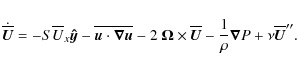
Assuming that there is no turbulence (
We see that Eq. (B.10) indicates that the pressure P is independent of x. The other Eq. (B.11), however, gives an explicit x-dependence for P. Therefore, we can conclude that unless there exists some sort of large-scale forcing to cancel the pressure gradient, there can be no equilibrium for this system. As noted by Leprovost & Kim (2008b), in the real physical situations phenomena like the thermal winds can balance the system.
References
- Balbus, S. A., & Hawley, J. F. 1991, ApJ, 376, 214 [NASA ADS] [CrossRef] (In the text)
- Balbus, S. A., & Hawley, J. F. 1998, RvMP, 70, 1 [NASA ADS] [CrossRef] (In the text)
- Blackman, E. G., & Field, G. B. 2002, PhRvL, 89, 265007 [NASA ADS] (In the text)
- Blackman, E. G., & Field, G. B. 2003, Phys. Fluids, 15, L73 [NASA ADS] [CrossRef]
-
Brandenburg, A. 2003, in Advances in nonlinear dynamos The Fluid
Mechanics of Astrophysics and Geophysics, ed. A. Ferriz-Mas, &
M. N
 ez (London and New York: Taylor & Francis), 9269
(In the text)
ez (London and New York: Taylor & Francis), 9269
(In the text) - Brandenburg, A., & Dobler, W. 2002, Comp. Phys. Comm., 147, 471 [NASA ADS] [CrossRef] (In the text)
- Brandenburg, A., & Subramanian, K. 2005, A&A, 439, 835 [NASA ADS] [CrossRef] [EDP Sciences] (In the text)
- Brandenburg, A., & Subramanian, K. 2007, AN, 328, 507 [NASA ADS] (In the text)
- Brandenburg, A., Moss, D., & Tuominen, I. 1992, A&A, 265, 328 [NASA ADS] (In the text)
- Brandenburg, A., Käpylä, P. J., & Mohammed, A. 2004, Phys. Fluids, 16, 1020 [NASA ADS] [CrossRef] (In the text)
- Brun, A. S., & Toomre, J. 2002, ApJ, 570, 865 [NASA ADS] [CrossRef] (In the text)
- Chan, K. L. 2001, ApJ, 548, 1102 [NASA ADS] [CrossRef] (In the text)
- Chandrasekhar, S. 1961, Hydrodynamic and Hydromagnetic stability (Oxford Univ. Press) (In the text)
- Elperin, T., Kleeorin, N., & Rogachevskii, I. 2003, PhRvE, 68, 016311 [NASA ADS] (In the text)
- Elperin, T., Golubev, I., Kleeorin, N., & Rogachevskii, I. 2007, PhRvE, 76, 066310 [NASA ADS]
- Fromang, S., Papaloizou, J., Lesur, G., & Heinemann, T. 2007, A&A, 476, 1123 [NASA ADS] [CrossRef] [EDP Sciences] (In the text)
- Garaud, P., & Ogilvie, G. I. 2005, JFM, 530, 145 [NASA ADS] [CrossRef] (In the text)
- Käpylä, P. J., & Brandenburg, A. 2007, AN, 328, 1006 [NASA ADS] (In the text)
- Käpylä, P. J., & Brandenburg, A. 2008, A&A, 488, 9 [NASA ADS] [CrossRef] [EDP Sciences] (In the text)
- Käpylä, P. J., Korpi, M. J., & Tuominen, I. 2004, A&A, 422, 793 [NASA ADS] [CrossRef] [EDP Sciences] (In the text)
- Käpylä, P. J., Mitra, D., & Brandenburg, A. 2009, PhRvE, 79, 016302 [NASA ADS] (In the text)
- Kitchatinov, L. L., & Rüdiger, G. 1993, A&A, 276, 96 [NASA ADS] (In the text)
- Kitchatinov, L. L., & Rüdiger, G. 2005, AN, 326, 379 [NASA ADS] (In the text)
- Kitchatinov, L. L., Pipin, V. V., & Rüdiger, G. 1994, AN, 315, 157 [NASA ADS] (In the text)
- Kleeorin, N., & Rogachevskii, I. 2006, PhRvE, 73, 046303 [NASA ADS] (In the text)
- Krause, F., & Rädler, K.-H. 1980, Mean-Field Magnetohydrodynamics and Dynamo Theory (Oxford: Pergamon Press) (In the text)
- Krause, F., & Rüdiger, G. 1974, AN, 295, 93 [NASA ADS] (In the text)
- Küker, M., Rüdiger, G., & Kitchatinov, L. L. 1993, A&A, 279, L1 [NASA ADS] (In the text)
- Leprovost, N., & Kim, E.-J. 2007, A&A, 463, 9L [NASA ADS] [CrossRef] (In the text)
- Leprovost, N., & Kim, E.-J. 2008a, PhRvE, 78, 016301 [NASA ADS]
- Leprovost, N., & Kim, E.-J. 2008b, PhRvE, 78, 036319 [NASA ADS] (In the text)
- Liljeström, A. J., Korpi, M. J., Käpylä, P. J., Brandenburg, A., & Lyra, W. 2009, AN, 330, 91 [NASA ADS] (In the text)
- Miesch, M. S., Brun, A. S., & Toomre, J. 2006, ApJ, 641, 618 [NASA ADS] [CrossRef] (In the text)
- Miesch, M. S., Brun, A. S., DeRosa, M. L., & Toomre, J. 2008, ApJ, 673, 557 [NASA ADS] [CrossRef]
- Miller, N., & Garaud, P. 2007, AIPC, 948, 165 [NASA ADS] (In the text)
- Mitra, D., Käpylä, P. J., Tavakol, R., & Brandenburg, A. 2009, A&A, 495, 1 [NASA ADS] [CrossRef] [EDP Sciences] (In the text)
- Ogilvie, G. I. 2003, MNRAS, 340, 969 [NASA ADS] [CrossRef] (In the text)
- Pessah, M. E., Chan, C.-K., & Psaltis, D. 2006, PhRvL, 97, 221103 [NASA ADS] (In the text)
- Pessah, M. E., Chan, C.-K., & Psaltis, D. 2008, MNRAS, 383, 683 [NASA ADS] (In the text)
- Pulkkinen, P., Tuominen, I., Brandenburg, A., Nordlund, Å., & Stein, R. F. 1993, A&A, 267, 265 [NASA ADS] (In the text)
- Rempel, M. 2005, ApJ, 622, 1320 [NASA ADS] [CrossRef] (In the text)
- Robinson, F. J., & Chan, K. L. 2001, MNRAS, 321, 723 [NASA ADS] [CrossRef] (In the text)
- Rüdiger, G. 1980, GAFD, 16, 239 [CrossRef] (In the text)
- Rüdiger, G. 1982, AN, 303, 293 [NASA ADS] (In the text)
- Rüdiger, G. 1989, Differential Rotation and Stellar Convection: Sun and Solar-type Stars (Berlin: Akademie Verlag) (In the text)
- Rüdiger, G. Egorov, P., & Ziegler, U. 2005, AN, 326, 315 [NASA ADS] (In the text)
- Schrinner, M., Rädler, K.-H., Schmitt, D., et al. 2005, AN, 326, 245 [NASA ADS] (In the text)
- Schrinner, M., Rädler, K.-H., Schmitt, D., et al. 2007, GAFD, 101, 81 [CrossRef]
- Shakura, N. I., & Sunyaev, R. A. 1973, A&A, 24, 337 [NASA ADS] (In the text)
- Spiegel, E. A., & Veronis, G. 1960, ApJ, 131, 442 [NASA ADS] [CrossRef] (In the text)
- Yousef, T. A., Brandenburg, A., & Rüdiger, G. 2003, A&A, 411, 321 [NASA ADS] [CrossRef] [EDP Sciences] (In the text)
- Yousef, T. A., Heinemann, T., Schekochihin, A. A., et al. 2008a, PhRvL, 100, 184501 [NASA ADS] (In the text)
- Yousef, T. A., Heinemann, T., Rincon, F., et al. 2008b, AN, 329, 737 [NASA ADS]
- Velikhov, E. P. 1959, Sov. Phys. JETP, 36, 1398 (In the text)
Online Material
Table B.1:
Summary of the runs with shear flow only. Here
![]() ,
and brackets around a quantity signify
that the number is not statistically significant.
,
and brackets around a quantity signify
that the number is not statistically significant.
Table B.2:
Summary of the runs in the Sets E and F with ![]() .
.
Footnotes
- ... rotation
- Tables B1-B3 are only available in electronic form at http://www.aanda.org
- ... ODE
- http://code.google.com/p/pencil-code/
All Tables
Table 1:
Summary of the different sets of simulations. The values
of ![]() ,
,
![]() ,
and
,
and ![]() are given in terms of
are given in terms of
![]() from a
run with
from a
run with
![]() .
.
Table B.1:
Summary of the runs with shear flow only. Here
![]() ,
and brackets around a quantity signify
that the number is not statistically significant.
,
and brackets around a quantity signify
that the number is not statistically significant.
Table B.2:
Summary of the runs in the Sets E and F with ![]() .
.
All Figures
| |
Figure 1:
Velocity component Uy, in the units of the sound speed,
from the Run B6 with
|
| Open with DEXTER | |
| In the text | |
| |
Figure 2:
Upper panel: turbulent viscosity divided by the molecular
viscosity for the simulation Sets A (solid line) and B (dashed line)
as a function of the Reynolds number. The dotted line, proportional
to |
| Open with DEXTER | |
| In the text | |
| |
Figure 3:
From top to bottom: Reynolds stress components Qxx,
Qyy, Qzz, and Qxy, normalised by
|
| Open with DEXTER | |
| In the text | |
| |
Figure 4: Same as Fig. 3 but for Set E, and different Strouhal numbers as indicated by the legend in the uppermost panel. |
| Open with DEXTER | |
| In the text | |
| |
Figure 5: Same as Fig. 4 but for the simulation Set F. |
| Open with DEXTER | |
| In the text | |
| |
Figure 6:
Upper panel: the two measures of the horizontal
|
| Open with DEXTER | |
| In the text | |
| |
Figure 7:
Left column:
|
| Open with DEXTER | |
| In the text | |
| |
Figure 8: Same as Fig. 7 but for the simulation Set H. |
| Open with DEXTER | |
| In the text | |
| |
Figure 9:
Nondiffusive contributions to the Reynolds stresses
parameterized by the coefficients
|
| Open with DEXTER | |
| In the text | |
| |
Figure 10: Same as Fig. 9 but for the simulation Set H. |
| Open with DEXTER | |
| In the text | |
| |
Figure 11:
Same as Fig. 4 but for a set of
runs with
|
| Open with DEXTER | |
| In the text | |
| |
Figure 12:
Upper panel: strouhal number from the triple correlations
as a function of |
| Open with DEXTER | |
| In the text | |
Copyright ESO 2009
Current usage metrics show cumulative count of Article Views (full-text article views including HTML views, PDF and ePub downloads, according to the available data) and Abstracts Views on Vision4Press platform.
Data correspond to usage on the plateform after 2015. The current usage metrics is available 48-96 hours after online publication and is updated daily on week days.
Initial download of the metrics may take a while.