| Issue |
A&A
Volume 505, Number 3, October III 2009
|
|
|---|---|---|
| Page(s) | 1199 - 1211 | |
| Section | Interstellar and circumstellar matter | |
| DOI | https://doi.org/10.1051/0004-6361/200912547 | |
| Published online | 18 August 2009 | |
C2H in prestellar cores
M. Padovani1,2 - C. M. Walmsley2 - M. Tafalla3 - D. Galli2 - H. S. P. Müller4
1 - Università di Firenze, Dipartimento di Astronomia e Scienza dello
Spazio, Largo E. Fermi 2, 50125 Firenze, Italy
2 -
INAF-Osservatorio Astrofisico di Arcetri, Largo E. Fermi 5, 50125
Firenze, Italy
3 -
Observatorio Astronómico Nacional, Alfonso XII 3, 28014 Madrid,
Spain
4 -
I. Physikalisches Institut, Universität zu Köln, Zülpicher
Straße 77, 50937 Köln, Germany
Received 20 May 2009 / Accepted 6 August 2009
Abstract
Aims. We study the abundance of
![]() in prestellar cores both because of its role in the chemistry and because it is a potential probe of the magnetic field. We also consider the non-LTE behaviour of the N=1-0 and N=2-1 transitions of
in prestellar cores both because of its role in the chemistry and because it is a potential probe of the magnetic field. We also consider the non-LTE behaviour of the N=1-0 and N=2-1 transitions of
![]() and improve current estimates of the spectroscopic constants of
and improve current estimates of the spectroscopic constants of
![]() .
.
Methods. We used the IRAM 30 m radiotelescope to map the N=1-0 and N=2-1 transitions of
![]() towards the prestellar cores L1498 and CB246. Towards CB246, we also mapped the 1.3 mm dust emission, the J=1-0 transition of
towards the prestellar cores L1498 and CB246. Towards CB246, we also mapped the 1.3 mm dust emission, the J=1-0 transition of
![]() and the J=2-1 transition of
and the J=2-1 transition of
![]() .
We used a Monte Carlo radiative transfer program to analyse the
.
We used a Monte Carlo radiative transfer program to analyse the
![]() observations of L1498. We derived the distribution of
observations of L1498. We derived the distribution of
![]() column densities and compared with the H2 column densities inferred from dust emission.
column densities and compared with the H2 column densities inferred from dust emission.
Results. We find that while non-LTE intensity ratios of different components of the N=1-0 and N=2-1 lines are present, they are of minor importance and do not impede
![]() column density determinations based upon LTE analysis. Moreover, the comparison of our Monte-Carlo calculations with observations suggest that the non-LTE deviations can be qualitatively understood. For extinctions less than 20 visual magnitudes, we derive toward these two cores (assuming LTE) a relative abundance [
column density determinations based upon LTE analysis. Moreover, the comparison of our Monte-Carlo calculations with observations suggest that the non-LTE deviations can be qualitatively understood. For extinctions less than 20 visual magnitudes, we derive toward these two cores (assuming LTE) a relative abundance [
![]() ]/[H2] of
]/[H2] of
![]() in L1498 and
in L1498 and
![]() in CB246 in reasonable agreement with our Monte-Carlo estimates. For L1498, our observations in conjunction with the Monte Carlo code imply a
in CB246 in reasonable agreement with our Monte-Carlo estimates. For L1498, our observations in conjunction with the Monte Carlo code imply a
![]() depletion hole of radius
depletion hole of radius
![]() cm similar to that found for other C-containing species. We briefly discuss the significance of the observed
cm similar to that found for other C-containing species. We briefly discuss the significance of the observed
![]() abundance distribution. Finally, we used our observations to provide improved estimates for the rest frequencies of all six components of the
abundance distribution. Finally, we used our observations to provide improved estimates for the rest frequencies of all six components of the
![]() (1-0) line and seven components of
(1-0) line and seven components of
![]() (2-1). Based on these results, we compute improved spectroscopic constants for
(2-1). Based on these results, we compute improved spectroscopic constants for
![]() .
We also give a brief discussion of the prospects for measuring magnetic field strengths using
.
We also give a brief discussion of the prospects for measuring magnetic field strengths using
![]() .
.
Key words: ISM: abundances - ISM: clouds - ISM: molecules - ISM: general - radio lines: ISM - molecular data
1 Introduction
The ethynyl radical
![]() is also of interest because hyperfine and spin interactions cause
the rotational transitions to split into as many as 11 components which
can be observed simultaneously with modern autocorrelation spectrometers.
This allows for a precise examination of the deviations from LTE in
individual rotational levels and eventually an evaluation of the
relative importance of collisional and radiative processes.
One can observe for example in the N=1-0 transition, at 3 mm, six
components
with line strengths varying by over an order of magnitude and whose
relative intensities
can be compared extremely precisely.
Departures from LTE have long plagued column density estimates in
molecular
lines which are often uncertain by a factor of order 2 as a
consequence. Reducing such uncertainties can only be achieved
by understanding the causes of non-LTE behaviour in level populations
and this requires both theoretical (calculations of collisional
rates) and observational work. In this study, we attempt
to delineate the problem in the case of
is also of interest because hyperfine and spin interactions cause
the rotational transitions to split into as many as 11 components which
can be observed simultaneously with modern autocorrelation spectrometers.
This allows for a precise examination of the deviations from LTE in
individual rotational levels and eventually an evaluation of the
relative importance of collisional and radiative processes.
One can observe for example in the N=1-0 transition, at 3 mm, six
components
with line strengths varying by over an order of magnitude and whose
relative intensities
can be compared extremely precisely.
Departures from LTE have long plagued column density estimates in
molecular
lines which are often uncertain by a factor of order 2 as a
consequence. Reducing such uncertainties can only be achieved
by understanding the causes of non-LTE behaviour in level populations
and this requires both theoretical (calculations of collisional
rates) and observational work. In this study, we attempt
to delineate the problem in the case of
![]() from an observational
point of view.
from an observational
point of view.
We have chosen to study two cores with contrasting properties. L1498
is a well studied core in the Taurus complex at a distance of 140 parsec
with a clear CO depletion hole. Its density structure has been
studied in detail
by Shirley et al. (2005) who conclude that their results are consistent with a
``Bonnor-Ebert sphere'' of central density
![]() cm-3 and
by Tafalla et al. (2004, 2006) who find a considerably higher central
density
of
cm-3 and
by Tafalla et al. (2004, 2006) who find a considerably higher central
density
of
![]() cm-3. Kirk et al. (2006) used SCUBA polarisation
measurements
to infer a surprisingly low value of the magnetic field of
cm-3. Kirk et al. (2006) used SCUBA polarisation
measurements
to infer a surprisingly low value of the magnetic field of ![]()
![]() G
in the plane of the sky.
Aikawa et al. (2005) modelled the molecular distribution and concluded
that their results were consistent with the contraction of a
``near equilibrium'' core. There is in general evidence for depletion of
C-bearing species such as c-C3H2 and C2S in a central
hole of
radius 1017 cm (Tafalla et al. 2006).
This is in contrast to NH3 and N2H+ which show no signs of
depletion
in the central high density region of the core.
G
in the plane of the sky.
Aikawa et al. (2005) modelled the molecular distribution and concluded
that their results were consistent with the contraction of a
``near equilibrium'' core. There is in general evidence for depletion of
C-bearing species such as c-C3H2 and C2S in a central
hole of
radius 1017 cm (Tafalla et al. 2006).
This is in contrast to NH3 and N2H+ which show no signs of
depletion
in the central high density region of the core.
CB246 (L1253) is a relatively isolated globule without an
associated IRAS source at a distance of 140-300 parsec
(Dame et al. 1987; Launhardt & Henning 1997) in the general direction of
the
Cepheus flare. For the purpose of this study, we adopt a distance of
200 pc.
CB246 is apparently a double core seen both in
NH3 and C2S
(Lemme et al. 1996; Codella & Scappini 1998) on a size scale of roughly
0.1 parsec.
The mass (dependent on the distance) is in the range 0.2-1 ![]() (Codella & Scappini 1998) from the NH3 maps, though there is
considerable uncertainty in this. From a chemical point of view, it is
interesting that there is rough general agreement between the spatial
distributions seen in NH3 and C2S. One aim of the present
observations has been to check if
(Codella & Scappini 1998) from the NH3 maps, though there is
considerable uncertainty in this. From a chemical point of view, it is
interesting that there is rough general agreement between the spatial
distributions seen in NH3 and C2S. One aim of the present
observations has been to check if
![]() shows signs of depletion towards
the peak emission seen in NH3.
shows signs of depletion towards
the peak emission seen in NH3.
In this article, we present IRAM 30 m maps of the emission in the N=1-0
transition of
![]() towards CB246 and L1498. We supplement this with
measurements at selected positions of the N=2-1 transition of
towards CB246 and L1498. We supplement this with
measurements at selected positions of the N=2-1 transition of
![]() as
well as maps of the 1.3 mm dust emission, the J=1-0 transition of
as
well as maps of the 1.3 mm dust emission, the J=1-0 transition of
![]() and the J=2-1 transition of
and the J=2-1 transition of
![]() towards CB246.
In Sect. 2, we describe our observational and data reduction procedures
and in Sect. 3, we summarise the observational results from the line measurements. In
Sect. 4,
we attempt to use our astronomical observations to estimate rest
frequencies
for the individual components of
towards CB246.
In Sect. 2, we describe our observational and data reduction procedures
and in Sect. 3, we summarise the observational results from the line measurements. In
Sect. 4,
we attempt to use our astronomical observations to estimate rest
frequencies
for the individual components of
![]() (1-0) and (2-1) and an updated
set of hyperfine parameters.
In Sect. 5, we give our conclusions concerning the deviations from
LTE populations for
(1-0) and (2-1) and an updated
set of hyperfine parameters.
In Sect. 5, we give our conclusions concerning the deviations from
LTE populations for
![]() as well as a very tentative interpretation.
In Sect. 6, we give our column density and abundance estimates in the
two objects and
discuss the evidence for depletion of
as well as a very tentative interpretation.
In Sect. 6, we give our column density and abundance estimates in the
two objects and
discuss the evidence for depletion of
![]() .
In Sect. 7, we discuss our results and in Sect. 8, we summarise our
conclusions.
.
In Sect. 7, we discuss our results and in Sect. 8, we summarise our
conclusions.
2 Observations
2.1 C2H in L1498 and CB246
The observations were carried out with the IRAM 30 m telescope. The
The two cores, L1498 and CB246, were mapped in
![]() (1-0) in 2008
in raster mode with a spacing of 20
(1-0) in 2008
in raster mode with a spacing of 20
![]() (channel spacing 20 kHz)
for L1498 and of 15
(channel spacing 20 kHz)
for L1498 and of 15
![]() for CB246 (thus close to Nyquist sampling for
CB246). In 2008, we also observed the
for CB246 (thus close to Nyquist sampling for
CB246). In 2008, we also observed the
![]() (2-1) line at the
positions given in Table 2. Finally in 2007, we observed
the
(2-1) line at the
positions given in Table 2. Finally in 2007, we observed
the
![]() (1-0) line towards the (0, 0) offset with 10 kHz resolution in
both sources.
(1-0) line towards the (0, 0) offset with 10 kHz resolution in
both sources.
The observed strategy was identical for all measurements:
frequency-switching mode
with a 7.5 MHz throw and a phase time of 0.5 s, with a calibration every 10 to 15 min.
The data were reduced using CLASS, the line data analysis program of the
GILDAS
software![]() .
Instrumental bandpass and atmospheric contributions were subtracted with
polynomial baselines,
before and after the folding of the two-phase spectra.
The final rms, in the main-beam temperature (
.
Instrumental bandpass and atmospheric contributions were subtracted with
polynomial baselines,
before and after the folding of the two-phase spectra.
The final rms, in the main-beam temperature (
![]() ),
in each channel of width
),
in each channel of width
![]() km s-1 is
km s-1 is
![]() mK for
both L1498 and CB246 and for both the N=1-0 and the N=2-1
transitions, while the system temperatures are
mK for
both L1498 and CB246 and for both the N=1-0 and the N=2-1
transitions, while the system temperatures are
![]() K
for the N=1-0 transition and
K
for the N=1-0 transition and
![]() K for the
N=2-1
transition.
In what follows, all temperatures are on the main-beam scale,
K for the
N=2-1
transition.
In what follows, all temperatures are on the main-beam scale,
![]() ,
where
,
where
![]() is the antenna temperature corrected for
atmospheric absorption,
and the forward and beam efficiencies are respectively
is the antenna temperature corrected for
atmospheric absorption,
and the forward and beam efficiencies are respectively
![]() and
and
![]() concerning the N=1-0 transition and
concerning the N=1-0 transition and
![]() and
and
![]() for the N=2-1 transition.
for the N=2-1 transition.
2.2 N2H+(1-0) and C18O(2-1) in CB246
Observations of the
![]() (1-0) multiplet (at 93 GHz) and
(1-0) multiplet (at 93 GHz) and
![]() (2-1) (at 219 GHz) in CB246 were carried out simultaneously
in July 2008,
with 3-4 mm pwv. The HPBW at the
(2-1) (at 219 GHz) in CB246 were carried out simultaneously
in July 2008,
with 3-4 mm pwv. The HPBW at the
![]() (1-0) and C18O(2-1)
frequencies are 26
(1-0) and C18O(2-1)
frequencies are 26
![]() and 11
and 11
![]() respectively.
The VESPA autocorrelator was used to obtain 10 kHz channel spacing
with 40 MHz bandwidth for N2H+(1-0) and 20 kHz channel
spacing with 40 MHz bandwidth for
respectively.
The VESPA autocorrelator was used to obtain 10 kHz channel spacing
with 40 MHz bandwidth for N2H+(1-0) and 20 kHz channel
spacing with 40 MHz bandwidth for
![]() (2-1). We observed using
the frequency-switching mode with a 7.5 MHz throw for N2H+(1-0) and a 15 MHz throw for
(2-1). We observed using
the frequency-switching mode with a 7.5 MHz throw for N2H+(1-0) and a 15 MHz throw for
![]() (2-1) and a phase time of 0.5 s with a calibration
every 10 to 15 min. We observed a region of
2.5 arcmin squared in extent with a spacing of 15
(2-1) and a phase time of 0.5 s with a calibration
every 10 to 15 min. We observed a region of
2.5 arcmin squared in extent with a spacing of 15
![]() .
Thus, the
N2H+ map is essentially Nyquist sampled whereas
.
Thus, the
N2H+ map is essentially Nyquist sampled whereas
![]() is under-sampled (though the maps shown subsequently are
smoothed to a resolution of 26
is under-sampled (though the maps shown subsequently are
smoothed to a resolution of 26
![]() ).
).
For N2H+, the final rms, in main-beam
temperature units (T![]() ), in channels of width
), in channels of width
![]() km s-1 was
km s-1 was
![]() mK, with a
mK, with a
![]() K. For
K. For
![]() ,
the final rms (channels
of width
,
the final rms (channels
of width
![]() km s-1) was
km s-1) was
![]() mK,
with a
mK,
with a
![]() K. The forward and the beam efficiencies
are respectively
K. The forward and the beam efficiencies
are respectively
![]() and
and
![]() for
for
![]() and
and
![]() and
and
![]() for
for
![]() .
.
2.3 Bolometer map of CB246
CB246 was observed in the 1.3 mm continuum with the IRAM 30 m telescope in May, November and December 2007. We used the MAMBO2 117-channel bolometer array in the on-the-fly mode with a scanning speed of 6
3 Observational results
3.1 C2H(1-0)
In Fig. 1, we show our map of the integrated intensity in the
The situation is rather different towards CB246 (see Fig. 2,
upper panel) where we see that the dust and
![]() emission have rather
similar distributions.
Both are double peaked, although the
emission have rather
similar distributions.
Both are double peaked, although the
![]() NW emission peak
is offset
about 30
NW emission peak
is offset
about 30
![]() to the south of its counterpart in dust emission whereas
towards the SE peak the difference is marginal.
to the south of its counterpart in dust emission whereas
towards the SE peak the difference is marginal.
![\begin{figure}
\par\resizebox{9cm}{!}{\includegraphics[angle=-90]{12547f1}}
\end{figure}](/articles/aa/full_html/2009/39/aa12547-09/img54.png) |
Figure 1:
Dust emission at 1.3 mm (after smoothing to 28
|
| Open with DEXTER | |
![\begin{figure}
\par\resizebox{9cm}{!}{\includegraphics[angle=-90]{12547f2}}
\end{figure}](/articles/aa/full_html/2009/39/aa12547-09/img55.png) |
Figure 2:
Upper panel: dust emission at 1.3 mm (after smoothing to
28
|
| Open with DEXTER | |
It is interesting to compare the distributions of different components.
We do this in Fig. 3 where we compare cuts in all the
1-0 component lines
with cuts in the continuum intensity. One sees that ratios of
different pairs of components do not vary greatly
along these cuts, although the ratio of the strong 87 316 MHz component
(No. 2 in
Table 4) to the weak 87284 MHz line (No. 1) at the L1498
dust peak
is somewhat smaller (about 45%) than elsewhere in the cut. However,
this ratio is always of order 3
as compared to the expected value of 10 for optically thin emission
(suggesting a moderately optically thick 87 316 MHz line).
There are thus indications of saturation of the stronger components of
the
![]() (1-0) line
and we conclude that optical depth effects are present but lines
have moderate opacities, as shown in Table 1 for selected positions
in the two observed sources.
It is noticeable also that while
(1-0) line
and we conclude that optical depth effects are present but lines
have moderate opacities, as shown in Table 1 for selected positions
in the two observed sources.
It is noticeable also that while
![]() has a minimum towards the dust
peak in L1498
(and we conclude this is a real column density minimum), there is a
little indication of
variation in the ratio of
has a minimum towards the dust
peak in L1498
(and we conclude this is a real column density minimum), there is a
little indication of
variation in the ratio of
![]() to dust continuum intensity crossing the
SE peak in CB246.
to dust continuum intensity crossing the
SE peak in CB246.
Table 1:
Line parametersa observed in
![]() (1-0)
(1-0)
![\begin{figure}
\par\resizebox{8.5cm}{!}{\includegraphics[angle=-90]{12547f3}}
\end{figure}](/articles/aa/full_html/2009/39/aa12547-09/img60.png) |
Figure 3:
Upper panels: continuum emission flux measured along the
NW-SE
cut in L1498,
see Fig. 1, and along the EW cut of the SE peak
in CB246,
see upper panel of Fig. 2.
Lower panels: ratio between the integrated intensity of the different
hyperfine components
of
|
| Open with DEXTER | |
Another indication of line transfer effects can be obtained from
comparing line profiles of the different
![]() (1-0) components as shown
in Fig. 4 where we show the high (10 kHz) spectral
resolution data from 2007.
It is noticeable that towards the dust peak, the weakest 87 407 MHz
component
(No. 5 in Table 4) has a maximum at a velocity where the
strong
87316 MHz line (No. 2) shows
a dip between two peaks. This is the signature expected for
``self-absorption''
by a foreground layer of density lower than that responsible for the bulk
of the emission.
The effect however is not sufficiently strong to change
the above conclusions concerning the importance of optical depth effects.
We note moreover that towards CB246, no effects of this type are seen.
(1-0) components as shown
in Fig. 4 where we show the high (10 kHz) spectral
resolution data from 2007.
It is noticeable that towards the dust peak, the weakest 87 407 MHz
component
(No. 5 in Table 4) has a maximum at a velocity where the
strong
87316 MHz line (No. 2) shows
a dip between two peaks. This is the signature expected for
``self-absorption''
by a foreground layer of density lower than that responsible for the bulk
of the emission.
The effect however is not sufficiently strong to change
the above conclusions concerning the importance of optical depth effects.
We note moreover that towards CB246, no effects of this type are seen.
| |
Figure 4:
Component 2 ( black), 3 ( green), 4 ( blue) and 5 ( red) of
|
| Open with DEXTER | |
3.2 C2H(2-1)
The
![]() (2-1) line has had little (if any) attention and it was thus interesting that we succeeded in detecting 7 of the 11 components of the line in both sources.
Line parameters are given in Table 2 and sample profiles are shown in
Fig. 5. It is interesting (see discussion below) that within the errors,
line intensities are consistent with LTE but that, in particular towards L1498,
the total optical depth derived from an LTE fit (see Table 2) is large and corresponds
to an optical depth of 3.1 in the strongest 174 663 MHz component (No. 2 of Table 5).
We note however that slight errors in rest frequencies could influence this
interpretation.
(2-1) line has had little (if any) attention and it was thus interesting that we succeeded in detecting 7 of the 11 components of the line in both sources.
Line parameters are given in Table 2 and sample profiles are shown in
Fig. 5. It is interesting (see discussion below) that within the errors,
line intensities are consistent with LTE but that, in particular towards L1498,
the total optical depth derived from an LTE fit (see Table 2) is large and corresponds
to an optical depth of 3.1 in the strongest 174 663 MHz component (No. 2 of Table 5).
We note however that slight errors in rest frequencies could influence this
interpretation.
![\begin{figure}
\par\mbox{\includegraphics[width=4.4cm,angle=0]{12547fg5a}\includegraphics[width=4.4cm,angle=0]{12547fg5b} }
\par
\end{figure}](/articles/aa/full_html/2009/39/aa12547-09/img62.png) |
Figure 5:
Hyperfine components of
|
| Open with DEXTER | |
Table 2:
Line parametersa observed in
![]() (2-1).
(2-1).
3.3 C18O and N2H+
In the lower panel of Fig. 2, we show a superposition
of our 1.3 mm continuum map (smoothed to an angular resolution of 26
![]() )
with the
)
with the
![]() (2-1) and the isolated component of
(2-1) and the isolated component of
![]() (1-0)
(
(1-0)
(
![]() )
integrated intensity maps,
together with the emission peaks in NH3(1,1), using the data obtained by
Lemme et al. (1996) and in C2S(21-10)
by Codella & Scappini (1998). There is a general similarity between the distributions of
)
integrated intensity maps,
together with the emission peaks in NH3(1,1), using the data obtained by
Lemme et al. (1996) and in C2S(21-10)
by Codella & Scappini (1998). There is a general similarity between the distributions of
![]() seen here and that of
seen here and that of
![]() (Fig. 2, upper panel).
In general, also the
(Fig. 2, upper panel).
In general, also the
![]() distribution resembles that seen in the continuum
but there are clear shifts (for example in the SE) between the peaks seen in the dust emission
and in
distribution resembles that seen in the continuum
but there are clear shifts (for example in the SE) between the peaks seen in the dust emission
and in
![]() .
In the NW, also the ``bar''-like structure seen in the continuum to be extended
N-S is also present in
.
In the NW, also the ``bar''-like structure seen in the continuum to be extended
N-S is also present in
![]() but seems even more elongated (dimensions of 100
but seems even more elongated (dimensions of 100
![]() in the continuum as compared to 120
in the continuum as compared to 120
![]() in
in
![]() ).
).
To the SE there is reasonable agreement between the continuum and
![]() intensity distributions and the ammonia peak appears to be consistent with these.
To the NW on the other hand, the continuum is extended in a ``bar''-like feature
and
intensity distributions and the ammonia peak appears to be consistent with these.
To the NW on the other hand, the continuum is extended in a ``bar''-like feature
and
![]() (but also
(but also
![]() )
peaks at the south end of this 40
)
peaks at the south end of this 40
![]() to the south of
the continuum peak. These differences suggest chemical differentiation in CB246 albeit
on a scale smaller than in L1498. Besides, the
to the south of
the continuum peak. These differences suggest chemical differentiation in CB246 albeit
on a scale smaller than in L1498. Besides, the
![]() peaks resemble the continuum structure
in the SE but differ considerably in the NW suggesting that in this case
(in contrast to L1498 and L1544, see Tafalla et al. 2006),
the
peaks resemble the continuum structure
in the SE but differ considerably in the NW suggesting that in this case
(in contrast to L1498 and L1544, see Tafalla et al. 2006),
the
![]() abundance may be varying with position.
The shift between the
abundance may be varying with position.
The shift between the
![]() NW peak and the continuum peak is
unusual, but not unprecedented (see Pagani et al. 2007).
However, a more detailed study of the radiative transfer and excitation
is needed to confirm this.
NW peak and the continuum peak is
unusual, but not unprecedented (see Pagani et al. 2007).
However, a more detailed study of the radiative transfer and excitation
is needed to confirm this.
In Fig. 6 we compare cuts in the strongest component of
![]() (1-0)
(component 2, see Table 4),
(1-0)
(component 2, see Table 4),
![]() (2-1) and the isolated component
of
(2-1) and the isolated component
of
![]() (1-0) with cuts in the continuum intensity.
(1-0) with cuts in the continuum intensity.
![]() and
and
![]() show a rather constant
line-to-continuum ratio in the SE peak cut, while in the NW peak cut, these molecules do not look
like the continuum structure, especially the
show a rather constant
line-to-continuum ratio in the SE peak cut, while in the NW peak cut, these molecules do not look
like the continuum structure, especially the
![]() emission which appears to be shifted down
compared to the continuum emission.
emission which appears to be shifted down
compared to the continuum emission.
![\begin{figure}
\par\resizebox{9cm}{!}{\includegraphics[angle=-90]{12547fg6}}
\end{figure}](/articles/aa/full_html/2009/39/aa12547-09/img64.png) |
Figure 6:
Upper panels: continuum emission flux measured along the SN cut of the SE
and the NW peaks in CB246, see upper panel of Fig. 2.
Lower panels: ratio between the integrated intensity of the component 2 of
|
| Open with DEXTER | |
3.4 Mass of CB246
In the continuum, CB246 shows a double-peaked profile, with a rounded SE clump with a radius (measured at half-power contour) of 33
![]() (corresponding to 0.03 pc at the distance of
200 pc) and a more elliptical NW clump with a major and a minor axes of 100
(corresponding to 0.03 pc at the distance of
200 pc) and a more elliptical NW clump with a major and a minor axes of 100
![]() (or 0.1 pc) and 44
(or 0.1 pc) and 44
![]() (or 0.04 pc), respectively. Dust emission is generally optically thin at millimetre wavelengths and hence is a direct tracer of the mass content of molecular cloud cores. In the hypothesis of an isothermal dust source, the total (dust plus gas) mass is related to the millimetre flux density, S1.3, integrated over the solid angle
(or 0.04 pc), respectively. Dust emission is generally optically thin at millimetre wavelengths and hence is a direct tracer of the mass content of molecular cloud cores. In the hypothesis of an isothermal dust source, the total (dust plus gas) mass is related to the millimetre flux density, S1.3, integrated over the solid angle
![]() according to the following equation
according to the following equation
 |
(1) |
where
To the south of the NW emission peak, there is a bright infrared source
(2MASS J23563433+5834043, see Fig. 2) which appears to be a
heavily reddened background star with visual extinction of ![]() 20 mag, consistent with our column density estimates.
20 mag, consistent with our column density estimates.
3.5 Gas kinematics
From the hyperfine fit of
![]() (1-0), using the rest frequencies discussed below (see Sect. 4.1), we derived the line center
velocities,
(1-0), using the rest frequencies discussed below (see Sect. 4.1), we derived the line center
velocities,
![]() ,
and in Fig. 7 we present the
radial profiles which are almost flat on the average, especially for
L1498. Radii
are computed with respect to the offset (0, 0) for the two sources (see
Figs. 1 and 2).
,
and in Fig. 7 we present the
radial profiles which are almost flat on the average, especially for
L1498. Radii
are computed with respect to the offset (0, 0) for the two sources (see
Figs. 1 and 2).
![\begin{figure}
\par\resizebox{8.8cm}{!}{\includegraphics[angle=-90]{12547fg7}}
\end{figure}](/articles/aa/full_html/2009/39/aa12547-09/img75.png) |
Figure 7:
Radial profile of line center velocity for L1498 ( upper panel)
and CB246 ( lower panel) derived from the hyperfine-structure fits of
|
| Open with DEXTER | |
Following Goodman et al. (1993), we checked for the presence of a
velocity gradient,
![]() ,
across these two cores using
,
across these two cores using
![]() (1-0) data. A further check has been done on CB246 using
(1-0) data. A further check has been done on CB246 using
![]() (1-0) and
(1-0) and
![]() (2-1) data, finding a good agreement within the errors with the
corresponding values from
(2-1) data, finding a good agreement within the errors with the
corresponding values from
![]() .
In Fig. 8 we show the local
velocity gradients in the two cores and in Table 3 we show
our results as regards the velocity gradient,
.
In Fig. 8 we show the local
velocity gradients in the two cores and in Table 3 we show
our results as regards the velocity gradient,
![]() ,
its
direction,
,
its
direction,
![]() and the mean LSR velocity,
and the mean LSR velocity,
![]() .
All these quantities are in good agreement
with the estimates of Goodman et al. (1993) and Tafalla et al. (2004) who
observed L1498 using NH3 and
.
All these quantities are in good agreement
with the estimates of Goodman et al. (1993) and Tafalla et al. (2004) who
observed L1498 using NH3 and
![]() as a tracer. Besides, we
evaluated the angular velocity,
as a tracer. Besides, we
evaluated the angular velocity, ![]() ,
assuming that the angular
velocity vector points in the direction given by
,
assuming that the angular
velocity vector points in the direction given by
![]() ,
that is
,
that is
![]() ,
where i is the inclination of
,
where i is the inclination of
![]() to the line of sight and the
position angle of
to the line of sight and the
position angle of
![]() is given by
is given by
![]() .
Statistically, for a random distribution of orientation,
.
Statistically, for a random distribution of orientation,
![]() (Chandrasekhar & Münch 1950;
Tassoul 1978).
To quantify the dynamic role of the rotation in a cloud, we calculated
the ratio between the rotational and the gravitational energy, denoted
with
(Chandrasekhar & Münch 1950;
Tassoul 1978).
To quantify the dynamic role of the rotation in a cloud, we calculated
the ratio between the rotational and the gravitational energy, denoted
with ![]() .
For a uniform density sphere,
.
For a uniform density sphere,
![]() ,
where R is the rotation radius, G the gravitational constant
and M the mass, and the specific angular momentum is defined as
,
where R is the rotation radius, G the gravitational constant
and M the mass, and the specific angular momentum is defined as
![]() .
.
| |
Figure 8:
|
| Open with DEXTER | |
The values of ![]() we found suggest that the clouds have little
rotational energy as generally found in molecular cloud cores (e.g.
Goodman et al. 1993). The specific angular momentum we evaluated for
these two cores is of order 10-3 km s-1 pc. In the hypothesis
that a core has been formed from a parental clump with equal mass and at
the same galactocentric distance of the core (about 7 kpc for L1498 and
CB246), we computed a rotation frequency of order 10-15 s-1
assuming that the angular momentum of the clump is due to Galactic
differential rotation (Clemens 1985).
This value corresponds to a specific angular momentum of
we found suggest that the clouds have little
rotational energy as generally found in molecular cloud cores (e.g.
Goodman et al. 1993). The specific angular momentum we evaluated for
these two cores is of order 10-3 km s-1 pc. In the hypothesis
that a core has been formed from a parental clump with equal mass and at
the same galactocentric distance of the core (about 7 kpc for L1498 and
CB246), we computed a rotation frequency of order 10-15 s-1
assuming that the angular momentum of the clump is due to Galactic
differential rotation (Clemens 1985).
This value corresponds to a specific angular momentum of
![]() km s-1 pc, that is 30 times greater than the L/M of the cores.
This shows that the specific angular momentum of the cores is low
compared to larger (galactic) scales. Thus angular momentum is lost in
forming cores as expected by Ohashi (1999) for cores with radius greater
than 0.03 pc. In particular, the cores lies on the relation founded by Ohashi (1999) for L/M as a function of the radius.
km s-1 pc, that is 30 times greater than the L/M of the cores.
This shows that the specific angular momentum of the cores is low
compared to larger (galactic) scales. Thus angular momentum is lost in
forming cores as expected by Ohashi (1999) for cores with radius greater
than 0.03 pc. In particular, the cores lies on the relation founded by Ohashi (1999) for L/M as a function of the radius.
Table 3: Results of gradient fitting.
Table 4:
Observed hyperfine structure components of the
![]() transition in
transition in
![]() :
rest frequenciesa, residuals
:
rest frequenciesa, residuals ![]() between observed and calculated frequenciesb,
and relative intensities f.
between observed and calculated frequenciesb,
and relative intensities f.
4 Evaluation of new spectroscopic parameters for C
 H
H
The C2H radical is a linear molecule. Its unpaired electron causes a splitting of
each rotational level into two fine structure levels. In addition, the spin of the
H nucleus causes each fine structure level to be split further into two hyperfine levels.
The strong transitions are those having
![]() which leads to four strong transitions at higher quantum numbers.
However, transitions with
which leads to four strong transitions at higher quantum numbers.
However, transitions with
![]() or with
or with
![]() ,
which have essentially vanishing intensities at high N,
may have fairly large relative intensities at lower values of N;
the only restriction which has to be followed strictly is
,
which have essentially vanishing intensities at high N,
may have fairly large relative intensities at lower values of N;
the only restriction which has to be followed strictly is
![]() or
or ![]() .
In the case of the N=1-0 and N=2-1 transitions, this leads to 6 and 11 hyperfine
lines, respectively, with non-zero intensity.
.
In the case of the N=1-0 and N=2-1 transitions, this leads to 6 and 11 hyperfine
lines, respectively, with non-zero intensity.
4.1 Rest frequencies
Previous rotational data of
![]() have been summarised by Müller et al. (2000).
They had measured submillimetre transitions up to 1 THz; the small hydrogen hyperfine splitting
was not resolved. Their data set also included 6 hyperfine lines of the N=1-0
measured toward a position north of Orion-KL (Gottlieb et al. 1983), four hyperfine components
of the N=2-1 transition obtained in the laboratory by the same authors
as well as four N=3-2 hyperfine features (Sastry et al. 1981).
These data as well as predictions are available from the recommended
CDMS
have been summarised by Müller et al. (2000).
They had measured submillimetre transitions up to 1 THz; the small hydrogen hyperfine splitting
was not resolved. Their data set also included 6 hyperfine lines of the N=1-0
measured toward a position north of Orion-KL (Gottlieb et al. 1983), four hyperfine components
of the N=2-1 transition obtained in the laboratory by the same authors
as well as four N=3-2 hyperfine features (Sastry et al. 1981).
These data as well as predictions are available from the recommended
CDMS![]() (Cologne Database for Molecular Spectroscopy, Müller et al. 2001,
2005).
(Cologne Database for Molecular Spectroscopy, Müller et al. 2001,
2005).
In the present investigation we have observed all six HFS components of the N=1-0 transition
as well as seven components of the N=2-1 transition. Because of good to very good signal-to-noise
(S/N) ratios of all these lines and because of the small line width it seemed promising
to determine improved rest frequencies for these lines with respect to those available
in the CDMS.
The main sources affecting the accuracy of rest frequencies, besides S/N and line width
are expected to be the symmetry of the (usually Gaussian) line shapes and the accuracy
with which the velocity structure of the source is known.
On the basis of the well determined rest frequencies of
![]() (1-0) (Pagani et al. 2009)
and
(1-0) (Pagani et al. 2009)
and
![]() (2-1) (Müller et al. 2001) we have derived at the dust continuum peak an LSR velocity of 7.80 km s-1 for L1498
based on the observations of these two transitions by Tafalla et al. (2002)
and an LSR velocity of -0.83 km s-1 for CB246 from the present observations
of these transitions (see Sect. 2.2).
Employing these LSR velocities, rest frequencies of
(2-1) (Müller et al. 2001) we have derived at the dust continuum peak an LSR velocity of 7.80 km s-1 for L1498
based on the observations of these two transitions by Tafalla et al. (2002)
and an LSR velocity of -0.83 km s-1 for CB246 from the present observations
of these transitions (see Sect. 2.2).
Employing these LSR velocities, rest frequencies of
![]() have been determined separately
for the two observed sources. They differ on average by 3 and 17 kHz, respectively,
for the N=1-0 and N=2-1 transition and the averages for each HFS component are given in
Tables 4 and 5, respectively together with the assignments,
the estimated uncertainties, the residuals
have been determined separately
for the two observed sources. They differ on average by 3 and 17 kHz, respectively,
for the N=1-0 and N=2-1 transition and the averages for each HFS component are given in
Tables 4 and 5, respectively together with the assignments,
the estimated uncertainties, the residuals ![]() between the observed frequencies
and those calculated from the final set of spectroscopic parameters,
and the relative intensities f.
between the observed frequencies
and those calculated from the final set of spectroscopic parameters,
and the relative intensities f.
Table 5:
Observed hyperfine structure components of the
![]() transition
in
transition
in
![]() :
rest frequenciesa, residuals
:
rest frequenciesa, residuals ![]() between observed and calculated frequenciesb,
and relative intensities f.
between observed and calculated frequenciesb,
and relative intensities f.
4.2 Spectroscopic parameters
These rest frequencies, together with previous laboratory values
(Sastry et al. 1981; Müller et al. 2000),
were used to calculate spectroscopic parameters for C2H. As in Müller et al. (2000),
the rotational constant B, the quartic and sextic distortion terms D and H,
the electron spin-rotation parameter ![]() along with its distortion correction
along with its distortion correction
![]() ,
as well as the scalar and tensorial electron spin-nuclear spin coupling terms
bF and c were determined. The distortion correction bFD to bF was not
determined with significance, even though its absolute uncertainty was slightly smaller than
in Müller et al. (2000), and it did not contribute significantly to the reduction of the
rms error. It was thus omitted from the final fit. However, it was found that
the 1H nuclear spin-rotation constant C improved the quality of the fit
by a non-negligible amount of 12% even though it was barely determined.
As, in addition, its value appeared to be reasonable, see
further below, this constant was retained in the final fit.
The resulting spectroscopic parameters are given in Table 6
together with the most recent previous values by Müller et al. (2000).
,
as well as the scalar and tensorial electron spin-nuclear spin coupling terms
bF and c were determined. The distortion correction bFD to bF was not
determined with significance, even though its absolute uncertainty was slightly smaller than
in Müller et al. (2000), and it did not contribute significantly to the reduction of the
rms error. It was thus omitted from the final fit. However, it was found that
the 1H nuclear spin-rotation constant C improved the quality of the fit
by a non-negligible amount of 12% even though it was barely determined.
As, in addition, its value appeared to be reasonable, see
further below, this constant was retained in the final fit.
The resulting spectroscopic parameters are given in Table 6
together with the most recent previous values by Müller et al. (2000).
Table 6: Spectroscopic parametersa (MHz) of C2H in comparison to previous values.
The most striking feature in the comparison of the present C2H rest frequencies with those from Gottlieb et al. (1983) is that the latter are on average 28.6 kHz higher in frequency, ranging from complete agreement to 51 kHz for the individual HFS components. Moreover, the deviations are a few times the uncertainties reported by Gottlieb et al. (1983) for some lines. In fact, employing the present spectroscopic parameters given in Table 6, the Gottlieb et al. (1983) data are reproduced to only 3.6 times their reported uncertainties on average. We suspect that the LSR velocity of the source north of Orion-KL used in Gottlieb et al. (1983) was not as well known as the authors assumed and that for the laboratory measurements the frequency determinations were slightly off or the estimates of the uncertainties were slightly too optimistic.
The present rest frequencies have been reproduced to 0.6 times the uncertainties,
slightly better still for the N=1-0 transition, suggesting that the uncertainties
in Table 5 and even more so in Table 4 have been judged
somewhat too conservatively. On the other hand, uncertainties in the LSR velocity
may justify such a conservative error estimate.
The N=3-2 lines from Sastry et al. (1981) have been reproduced to better than 18 kHz,
which is much better than the ![]() 45 kHz with which these data where reproduced
in Müller et al. (2000). In other words, these N=3-2 rest frequencies are
much better compatible with the present N=1-0 and N=2-1 rest frequencies
than with those from Gottlieb et al. (1983). The submillimetre data from
Müller et al. (2000) are
at somewhat higher frequencies and quantum numbers such that both present and
previous spectroscopic parameters in Table 6 reproduce these data
on average to about 0.6 times the reported uncertainties.
45 kHz with which these data where reproduced
in Müller et al. (2000). In other words, these N=3-2 rest frequencies are
much better compatible with the present N=1-0 and N=2-1 rest frequencies
than with those from Gottlieb et al. (1983). The submillimetre data from
Müller et al. (2000) are
at somewhat higher frequencies and quantum numbers such that both present and
previous spectroscopic parameters in Table 6 reproduce these data
on average to about 0.6 times the reported uncertainties.
While frequency deviations of a few tens of kHz may possibly be neglected in
observations of hot cores or similar sources, the deviations are rather considerable
for investigations into the dynamics of dark clouds as in the present study.
The deviations are also reflected in the small (![]() 11 kHz) differences in the
rotational constant B, see Table 6. Nevertheless, these
deviations are more than four times the combined uncertainties and thus clearly significant.
It is worth noting that the B value in Müller et al. (2000) is determined essentially by
the data from Gottlieb et al. (1983). The slightly higher D value from the present study,
just outside the combined uncertainties, compensates the change in B to some degree
for the submillimetre lines. The sextic term H is essentially the same as in
the previous study, still not determined with significance, but probably of the
right order of magnitude.
11 kHz) differences in the
rotational constant B, see Table 6. Nevertheless, these
deviations are more than four times the combined uncertainties and thus clearly significant.
It is worth noting that the B value in Müller et al. (2000) is determined essentially by
the data from Gottlieb et al. (1983). The slightly higher D value from the present study,
just outside the combined uncertainties, compensates the change in B to some degree
for the submillimetre lines. The sextic term H is essentially the same as in
the previous study, still not determined with significance, but probably of the
right order of magnitude.
Changes in the fine structure parameters and in the larger hyperfine structure
parameters are essentially insignificant. The distortion correction bFD
had been used in the previous fit of Müller et al. (2000) since its inclusion improved the
Gottlieb et al. (1983) data to be reproduced on average from 1.31 times the uncertainties
to 0.93 times the uncertainties. In present trial fits its value was determined
as
-0.0021 (33) MHz. The magnitude of the ratio bFD/bF is now much closer
to that of
![]() ,
but still much bigger than that of D/B.
However, the uncertainty was larger in magnitude than the value, and the inclusion of
the parameter in the fit improved the quality of the fit only insignificantly.
The term bFD was consequently omitted from the final fit.
The inclusion of the 1H nuclear spin-rotation term C in the present fit
requires some explanation. This term is usually small and negative and frequently
scaling with the rotational constant is the dominant contribution to its size.
The C2H value of -8.7 (53) kHz agrees within its large uncertainty
with the experimental one of -4.35 (5) kHz for HCN
(Ebenstein & Muenter 1984)
and with the calculated values of -4.80 kHz and -5.55 kHz for HCN and
HCO+ (Schmid-Burgk et al. 2004) and appears thus to be reasonable as these species have
fairly similar rotational constants.
,
but still much bigger than that of D/B.
However, the uncertainty was larger in magnitude than the value, and the inclusion of
the parameter in the fit improved the quality of the fit only insignificantly.
The term bFD was consequently omitted from the final fit.
The inclusion of the 1H nuclear spin-rotation term C in the present fit
requires some explanation. This term is usually small and negative and frequently
scaling with the rotational constant is the dominant contribution to its size.
The C2H value of -8.7 (53) kHz agrees within its large uncertainty
with the experimental one of -4.35 (5) kHz for HCN
(Ebenstein & Muenter 1984)
and with the calculated values of -4.80 kHz and -5.55 kHz for HCN and
HCO+ (Schmid-Burgk et al. 2004) and appears thus to be reasonable as these species have
fairly similar rotational constants.
5 Non-LTE hyperfine populations
In this section we consider the evidence for non-LTE populations in the
hyperfine levels
sampled by our observations.
We first compare the observed intensity ratios of
![]() in L1498 and CB246 with the predictions of simple LTE models and find
that while real deviations
from LTE populations are present, the LTE assumption is an approximation
which is useful for many purposes.
We then consider a Monte Carlo radiative transfer program for the case of
in L1498 and CB246 with the predictions of simple LTE models and find
that while real deviations
from LTE populations are present, the LTE assumption is an approximation
which is useful for many purposes.
We then consider a Monte Carlo radiative transfer program for the case of
![]() and show that the observed deviations can be approximately understood
with an educated guess
at the (unknown)
and show that the observed deviations can be approximately understood
with an educated guess
at the (unknown)
![]() collisional rates.
collisional rates.
5.1 Single- and two-layer models
We note first that for the case of LTE between different hyperfine levels
(i.e. all transitions of a given multiplet have the same excitation
temperature),
we expect that for a homogeneous slab, the ratio of line intensities of
two transitions Rij is given by:
where
Figure 10 shows analogous results for
![]() (2-1).
There are fewer positions but again, we see significant deviations from
the homogeneous single layer prediction of Eq. (2). The ratio R32 (upper left panel) of the 174 667 and 174 663 MHz lines is
typically between 0.5 and 0.6 as compared to the optically thin LTE
prediction of 0.66. These differences are small but appear to be
significant.
(2-1).
There are fewer positions but again, we see significant deviations from
the homogeneous single layer prediction of Eq. (2). The ratio R32 (upper left panel) of the 174 667 and 174 663 MHz lines is
typically between 0.5 and 0.6 as compared to the optically thin LTE
prediction of 0.66. These differences are small but appear to be
significant.
Equation (2) assumes a homogeneous one-dimensional solution of the transfer equation and it is clear that for a real prestellar core, gradients in both temperature and density are present. Indeed observations of some cores in strong ground state transitions such as HCO+(1-0) are complicated by absorption in a foreground layer whose excitation appears to be essentially that of the cosmic background (Tafalla et al. 1998).
In the particular case of
![]() towards L1498, the ``self-absorption'' observed in the
87 316 MHz line (see Fig. 4) suggests that something of this sort may occur also for
towards L1498, the ``self-absorption'' observed in the
87 316 MHz line (see Fig. 4) suggests that something of this sort may occur also for
![]() . In view of this, we have also considered a two-layer model of the type discussed by Myers et al. (1996) with background (b) and foreground (f) layers having excitation temperatures
. In view of this, we have also considered a two-layer model of the type discussed by Myers et al. (1996) with background (b) and foreground (f) layers having excitation temperatures
![]() and
and
![]() and the optical depths
and the optical depths ![]() and
and ![]() respectively. We then find for the emergent intensity of ith component:
respectively. We then find for the emergent intensity of ith component:
where
is the Planck-corrected brightness temperature and
![\begin{displaymath}\phi_{i}=2\sqrt{\frac{\ln2}{\pi}}\exp\left\{-\frac{4[V-(-1)^{m}\langle V_{k,i}\rangle]^{2}\ln2}{\sigma^{2}}\right\}
\end{displaymath}](/articles/aa/full_html/2009/39/aa12547-09/img137.png) |
(5) |
with m=0 for the foreground layer and m=1 for the background layer. We have included in Figs. 9 and 10 predictions based on our two-layer model varying
![\begin{figure}
\par\resizebox{9cm}{!}{\includegraphics[angle=0]{12547fg9}}
\end{figure}](/articles/aa/full_html/2009/39/aa12547-09/img140.png) |
Figure 9:
Ratio of the integrated intensities of some couples of components of
|
| Open with DEXTER | |
![\begin{figure}
\par\resizebox{8.8cm}{!}{\includegraphics[angle=0]{12547fg10}}
\end{figure}](/articles/aa/full_html/2009/39/aa12547-09/img141.png) |
Figure 10:
Ratio of the integrated intensities of some couples of components of
|
| Open with DEXTER | |
5.2 Monte Carlo treatment of radiative transfer in the C2H rotational transitions
The two-layer model, with its
assumption of the same excitation temperature for all
hyperfine components in each layer and its
discontinuous jump in conditions between the two emitting regions,
misses an important
part of the complex pattern of level populations responsible for
the emission in
![]() (1-0).
As can be seen in Fig. 4, the hyperfine components
of C2H(1-0) are simultaneously subthermal and optically thick
in both L1498 and CB246, and under these conditions, the excitation
temperature of each component is determined by a delicate
balance between collisions and trapping. This balance will be different
for each transition depending on its particular optical depth,
and it will therefore give rise to differences in excitation
between the components of the N=1-0 multiplet.
The large optical depth of the lines, in addition, makes the emission
from each component originate in gas at different depth in the core,
and this also contributes to differences in the observed line intensities.
Such complex interplay between excitation and
optical depth effects cannot be treated accurately with the two-layer
model, and its analysis requires a more sophisticated numerical scheme.
In this Section, we present the result of a (partial) solution to
the C2H radiative transfer problem using the same Monte Carlo code
used in Tafalla et al. (2004, 2006) to analyse the emission from
a number of molecular species in the L1498 and L1517B cores.
(1-0).
As can be seen in Fig. 4, the hyperfine components
of C2H(1-0) are simultaneously subthermal and optically thick
in both L1498 and CB246, and under these conditions, the excitation
temperature of each component is determined by a delicate
balance between collisions and trapping. This balance will be different
for each transition depending on its particular optical depth,
and it will therefore give rise to differences in excitation
between the components of the N=1-0 multiplet.
The large optical depth of the lines, in addition, makes the emission
from each component originate in gas at different depth in the core,
and this also contributes to differences in the observed line intensities.
Such complex interplay between excitation and
optical depth effects cannot be treated accurately with the two-layer
model, and its analysis requires a more sophisticated numerical scheme.
In this Section, we present the result of a (partial) solution to
the C2H radiative transfer problem using the same Monte Carlo code
used in Tafalla et al. (2004, 2006) to analyse the emission from
a number of molecular species in the L1498 and L1517B cores.
As the modelling of the L1498 emission in Tafalla et al. (2004, 2006)
already fixed the physical description of this
core (radial profiles of density, temperature, and
velocity), the only parameter left free to model
the C2H emission is the radial profile of abundance.
Unfortunately, the C2H analysis
is limited due to the lack of known collision rates for the
species, and this forces us to make an educated guess of
this important set of coefficients. Following Turner et al. (1999),
we approximate the collision rates of C2H using
those for HCN calculated by Green & Thaddeus (1974). From these rates,
which do not include hyperfine structure, we derive a new
set of rates with hyperfine structure assuming that the
new rates are simply proportional to the degeneracy of the
final state (Guilloteau & Baudry 1981; Lique et al. 2009).
Additional
![]() rates were included by following the recipe from
Turner et al. (1999), and
a total of 30 levels with 37 transitions (up to N=7
and an energy equivalent to 120 K) were used in the calculation.
rates were included by following the recipe from
Turner et al. (1999), and
a total of 30 levels with 37 transitions (up to N=7
and an energy equivalent to 120 K) were used in the calculation.
Following the analysis of other species in L1498,
the goal of our C2H modeling was to fit simultaneously
the combined radial profile of N=1-0 integrated intensity
together with the central spectra of the different components of
the N=1-0 and N=2-1 multiplets, assuming a uniform kinetic
temperature of 10 K (as derived from a non-LTE analysis of the
NH3 data by Tafalla et al. 2004). A first set of model runs
using the collision rates described before
predicted excitation temperatures that were too high
in the outer core layers, a situation that is
inconsistent with the self absorbed profile seen in the
thickest N=1-0 component (Fig. 4).
This inconsistency indicated that the guessed C2H
collision rates were too large, and that they should
be significantly reduced in order to match the observations.
To avoid introducing artifacts in the relative excitation
of the hyperfine components, the collision rates were reduced
dividing
them by a global factor of 3. With these corrected collision rates,
a fit was achieved by assuming a constant C2H abundance
with respect to H2of
![]() and a central depletion region of radius
and a central depletion region of radius
![]() cm inside which the
cm inside which the
![]() abundance is
negligible (10-4 times the outer value),
similar to that of other species
in L1498, see Tafalla et al. (2006). The results of this model
are shown in Fig. 11 (red lines) superposed to
observations (black
histograms and squares). As it can be seen, the model fits reasonably well
both the radial profile of N=1-0 intensity and the spectra of
most components in both the N=1-0 and N=2-1 multiplets.
The model in addition, fits reasonably well
the observed ratios of line pairs presented in Fig. 9.
abundance is
negligible (10-4 times the outer value),
similar to that of other species
in L1498, see Tafalla et al. (2006). The results of this model
are shown in Fig. 11 (red lines) superposed to
observations (black
histograms and squares). As it can be seen, the model fits reasonably well
both the radial profile of N=1-0 intensity and the spectra of
most components in both the N=1-0 and N=2-1 multiplets.
The model in addition, fits reasonably well
the observed ratios of line pairs presented in Fig. 9.
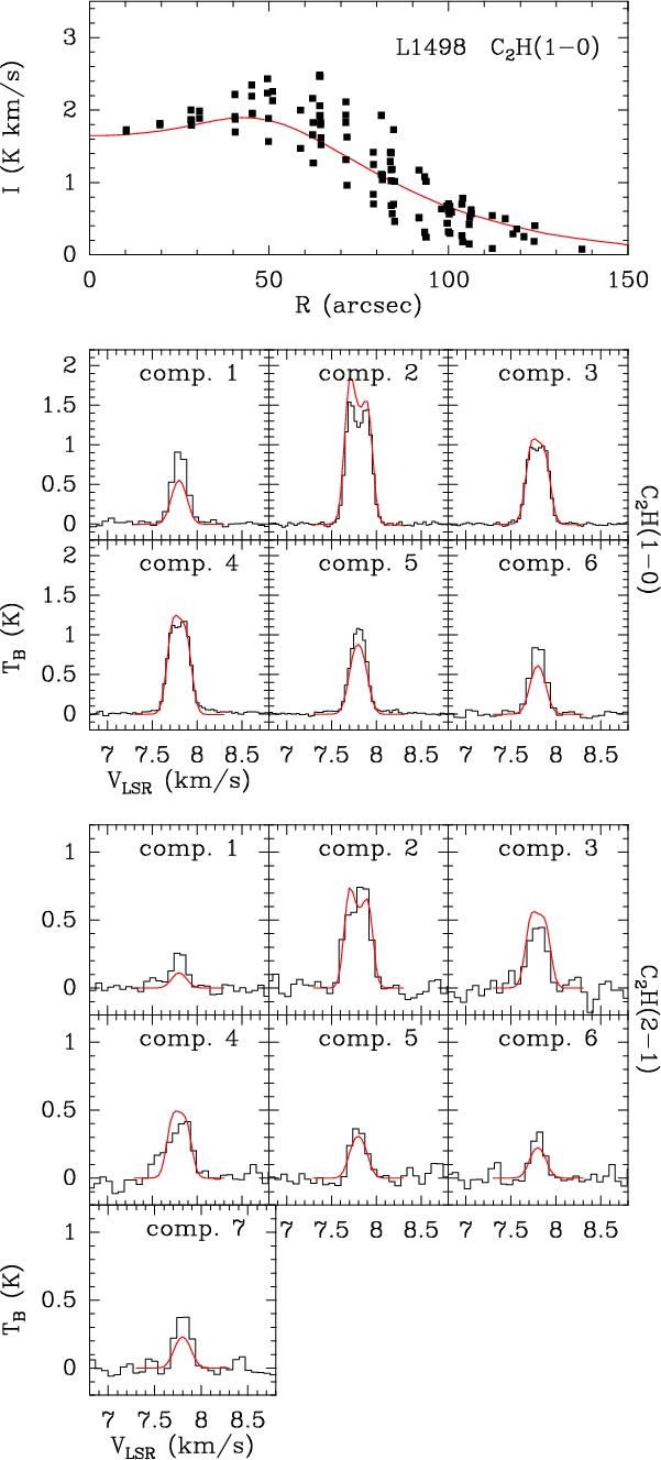 |
Figure 11: Comparison between observations and our best fit Monte Carlo model of the C2H emission in L1498. Top panel: radial profile of observed C2H(1-0) intensity integrated over all hyperfine components ( filled squares) and model prediction for a constant abundance core with a central depletion hole ( solid red line). Middle panels: emerging spectra for each component of the C2H(1-0) multiplet ( black histograms) and predictions for the same best fit model ( solid red lines). Bottom panels: same as middle panels but for the components of the C2H(2-1) multiplet. Note the reasonably good fit of all observables despite the use of highly approximated collisional rates (see text). |
| Open with DEXTER | |
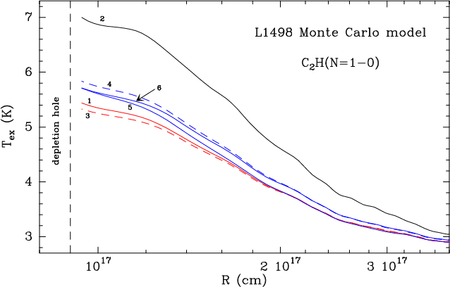 |
Figure 12: Radial profile of excitation temperature for each hyperfine component of C2H(1-0) as predicted by our best fit Monte Carlo model (each component is labelled according to the ordering in Table 3). Note the gradual drop of Tex with radius, which is caused by the combined decrease in collisional excitation and photon trapping towards the outer core. The different hyperfine components have different Tex depending mostly on trapping effects (see text for a full discussion). |
| Open with DEXTER | |
If our Monte Carlo model fits the
observed C2H emission, we can
use it to analyze the excitation of the different
N=1-0 components and understand
the origin of the observed line ratios. This is best done
by studying the radial profile of excitation temperature,
which is presented in Fig. 12.
As the figure shows, the
![]() of each component
systematically decreases with radius,
from about 6 K in the core interior to a value close to
the cosmic background temperature
near the core edge. The figure, in addition, shows that
at each radius, the
of each component
systematically decreases with radius,
from about 6 K in the core interior to a value close to
the cosmic background temperature
near the core edge. The figure, in addition, shows that
at each radius, the
![]() of the different components can differ
by as much as 1 K, and that component 2 is significantly
more excited than the rest. These differences in excitation
over the core and among components
could in principle result from differences in the
contribution of collisions or from photon trapping, and
to disentangle the two effects
we have run an alternative model having
a factor of 104 lower abundance. This optically
thin case also presents an outward drop in
of the different components can differ
by as much as 1 K, and that component 2 is significantly
more excited than the rest. These differences in excitation
over the core and among components
could in principle result from differences in the
contribution of collisions or from photon trapping, and
to disentangle the two effects
we have run an alternative model having
a factor of 104 lower abundance. This optically
thin case also presents an outward drop in
![]() ,
this time entirely due to the effect of collisions,
but it predicts excitation temperatures in the core interior that
are about 1 K lower than for the best fit model.
In addition,
component 2 in this thin case has a
,
this time entirely due to the effect of collisions,
but it predicts excitation temperatures in the core interior that
are about 1 K lower than for the best fit model.
In addition,
component 2 in this thin case has a
![]() comparable to that of the other components,
and the overall scatter of
comparable to that of the other components,
and the overall scatter of
![]() among all components does not exceed
0.5 K. This decrease in the excitation
when the lines become thin indicates that
in the best fit model
the N=1 level populations are significantly enhanced by trapping
of N=1-0 photons. The higher excitation of component 2,
in particular, appears as an extreme case of trapping:
this component has the largest relative intensity
and therefore is the most sensitive one to optical depth effects.
Its sensitivity to trapping makes it
the brightest line of the multiplet despite
suffering from self absorption at the line centre.
Differential line trapping seems also responsible
for the different intensity of components 3 and 4, which would
otherwise be equally bright
because of their equal Einstein A coefficient and upper
level statistical weight. As Fig. 12 shows, component 4
has an
among all components does not exceed
0.5 K. This decrease in the excitation
when the lines become thin indicates that
in the best fit model
the N=1 level populations are significantly enhanced by trapping
of N=1-0 photons. The higher excitation of component 2,
in particular, appears as an extreme case of trapping:
this component has the largest relative intensity
and therefore is the most sensitive one to optical depth effects.
Its sensitivity to trapping makes it
the brightest line of the multiplet despite
suffering from self absorption at the line centre.
Differential line trapping seems also responsible
for the different intensity of components 3 and 4, which would
otherwise be equally bright
because of their equal Einstein A coefficient and upper
level statistical weight. As Fig. 12 shows, component 4
has an ![]() 0.5 K higher
0.5 K higher
![]() in the
inner core, and this is most likely the result of enhanced
trapping due to an overpopulation of the
N,J,F=0,1/2,1level, where most N=1-0 transitions end (except for
components 3 and 6).
in the
inner core, and this is most likely the result of enhanced
trapping due to an overpopulation of the
N,J,F=0,1/2,1level, where most N=1-0 transitions end (except for
components 3 and 6).
In summary, our model shows that most excitation ``anomalies'' of the hyperfine components in the N=1-0 multiplet can be explained as resulting from the different balance between collisions and trapping expected for lines of very different intrinsic intensities under conditions of subthermal excitation and high optical depth. Further work on this issue requires an improved set of collision rates for C2H, and we encourage collision rate modelers to consider this species for future computations.
6 Column density and abundance estimate
Deriving a column density for C2H requires an estimate of the excitation temperature. This as we see in the Monte Carlo calculations discussed above depends on the line transfer and hence on position within the core. However a reasonable approximation to the column density can be obtained assuming a homogeneous layer with constant excitation temperature. We have verified this assumption for the case of L1498 using the Monte Carlo program.
The excitation temperature
![]() can be inferred (method 1) from an LTE fit to the hyperfine
components of either the N=1-0 or N=2-1 lines assuming unity beam filling factor
and using the measured intensity of optically thick transitions. An independent
measure can be obtained (method 2) from the ratio of intensities of low line strength
transitions of the N=2-1 and N=1-0 lines assuming them to be optically thin.
We summarize in Table 7 the excitation temperatures derived
using these different approaches for
the positions where we have N=2-1 data available. From Table 7 we see that
in both sources, the excitation temperature appears to be between 3.8 and 4.9 K. We will assume an excitation temperature of 4 K in the following for
all positions.
can be inferred (method 1) from an LTE fit to the hyperfine
components of either the N=1-0 or N=2-1 lines assuming unity beam filling factor
and using the measured intensity of optically thick transitions. An independent
measure can be obtained (method 2) from the ratio of intensities of low line strength
transitions of the N=2-1 and N=1-0 lines assuming them to be optically thin.
We summarize in Table 7 the excitation temperatures derived
using these different approaches for
the positions where we have N=2-1 data available. From Table 7 we see that
in both sources, the excitation temperature appears to be between 3.8 and 4.9 K. We will assume an excitation temperature of 4 K in the following for
all positions.
Table 7:
Values of
![]() [K] derived using the two
methods.
[K] derived using the two
methods.
For an optically thin
![]() (1-0) line, one can
derive the column density,
(1-0) line, one can
derive the column density,
![]() ,
through the formula:
,
through the formula:
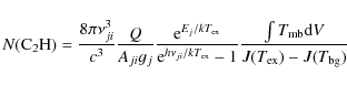
where
We need to compare this with the molecular hydrogen column density N(H2) and we do this using the mm dust emission (from Tafalla et al. 2004, for L1498 and from this work, see Sect. 2.3, for CB246). We assume here in both sources a dust grain opacity of 0.005 cm2 g-1 of dust and a dust temperature of 10 K, as in Sect. 3.4.
We also evaluated the column densities and the abundances of
![]() and CO
for CB246 (using our data, see Sect. 2.2) and for L1498
(using data from Tafalla et al. 2004). We derived N(
and CO
for CB246 (using our data, see Sect. 2.2) and for L1498
(using data from Tafalla et al. 2004). We derived N(
![]() )
following
the same procedure as for N(
)
following
the same procedure as for N(
![]() ). Thus, if the stronger components
of
). Thus, if the stronger components
of
![]() (1-0) are thick then we integrated only over the isolated component
(
(1-0) are thick then we integrated only over the isolated component
(
![]() ), dividing the result by
its line strength (0.111). In the case of
), dividing the result by
its line strength (0.111). In the case of
![]() ,
we used directly
Eq. (6) to calculate N(
,
we used directly
Eq. (6) to calculate N(
![]() )
and N(CO) assuming [16O]/[18O]
)
and N(CO) assuming [16O]/[18O] ![]() 560
(Wilson & Rood 1994). We give in Table 8 abundance estimates
that we have made at selected positions in L1498 and CB246.
560
(Wilson & Rood 1994). We give in Table 8 abundance estimates
that we have made at selected positions in L1498 and CB246.
Table 8: Molecular abundances in L1498 and CB246.
In Fig. 13, we show the plot of
![]() ,
,
![]() and CO column
density against H2 column density at different positions in both
sources.
We find that for column densities
N(H2)
and CO column
density against H2 column density at different positions in both
sources.
We find that for column densities
N(H2) ![]()
![]() cm-2, N(
cm-2, N(
![]() )
is
proportional to
N(H2) but, in L1498, for higher values of N(H2), this
proportionality breaks
down and N(
)
is
proportional to
N(H2) but, in L1498, for higher values of N(H2), this
proportionality breaks
down and N(
![]() )
seems to saturate at a value of
)
seems to saturate at a value of ![]()
![]() cm-2. This
is likely due to depletion of
cm-2. This
is likely due to depletion of
![]() in the high density core of L1498 as already
suggested by the maps in Fig. 1, the cuts in Fig. 3 and the Monte Carlo modeling.
This behaviour is in complete analogy with
several other species including the carbon rich molecule C3H2
(Tafalla et al. 2006).
in the high density core of L1498 as already
suggested by the maps in Fig. 1, the cuts in Fig. 3 and the Monte Carlo modeling.
This behaviour is in complete analogy with
several other species including the carbon rich molecule C3H2
(Tafalla et al. 2006).
On the other hand, for N(H2) less than
![]() cm-2, we
find that the ratio N(
cm-2, we
find that the ratio N(
![]() )/N(H2) is constant corresponding to a constant
)/N(H2) is constant corresponding to a constant
![]() abundance in the low density part of the core. This corresponds to
an average estimated
abundance in the low density part of the core. This corresponds to
an average estimated
![]() abundance relative to H2 of
abundance relative to H2 of
![]() in L1498 and
in L1498 and
![]() in
CB246. Our
in
CB246. Our
![]() abundances estimate for L1498 using Eq. (6)
agrees to within 20% with the Monte-Carlo estimate discussed in Sect. 5.2.
It is noteworthy and somewhat surprising to us that the
abundances estimate for L1498 using Eq. (6)
agrees to within 20% with the Monte-Carlo estimate discussed in Sect. 5.2.
It is noteworthy and somewhat surprising to us that the
![]() abundances are so similar
in cores of differing characteristics.
abundances are so similar
in cores of differing characteristics.
A more strict correlation over the whole range of observed H2 column density
is shown by the ratio N(
![]() )/N(H2) which corresponds to an average estimated
)/N(H2) which corresponds to an average estimated
![]() abundance relative to H2 of
abundance relative to H2 of
![]() in L1498
and
in L1498
and
![]() in CB246.
in CB246.
![]() behaves differently showing
a rather constant value of its column density over the N(H2) range corresponding
to N(CO) =
behaves differently showing
a rather constant value of its column density over the N(H2) range corresponding
to N(CO) =
![]() cm-2 in L1498 and
cm-2 in L1498 and
![]() cm-2 in CB246, while the average abundance relative to
H2 is
cm-2 in CB246, while the average abundance relative to
H2 is
![]() in L1498 and
in L1498 and
![]() in CB246.
in CB246.
One difference between CB246 and L1498 is that the
![]() peak
(see Fig. 13) is a factor 1.33 smaller
in CB246 and indeed does not reach values for which large depletion is
noted in L1498. However, our map in
peak
(see Fig. 13) is a factor 1.33 smaller
in CB246 and indeed does not reach values for which large depletion is
noted in L1498. However, our map in
![]() (2-1) (see lower panel of Fig. 2) as
well as the cuts shown in Fig. 6 suggest to us that some CO depletion
does occur in CB246.
(2-1) (see lower panel of Fig. 2) as
well as the cuts shown in Fig. 6 suggest to us that some CO depletion
does occur in CB246.
![\begin{figure}
\par\resizebox{8.5cm}{!}{\includegraphics[angle=0]{12547fg13}}
\end{figure}](/articles/aa/full_html/2009/39/aa12547-09/img195.png) |
Figure 13:
Plot of the column density of
|
| Open with DEXTER | |
7 Discussion
In this study, we have compared two cores of rather different
characteristics. L1498 is embedded in the Taurus complex with a
total dimension of
![]() arcmin (Caselli et al. 2002) corresponding to
arcmin (Caselli et al. 2002) corresponding to
![]() pc at the distance of 140 parsec (Elias 1978). CB246 is an isolated globule with dimensions
of
pc at the distance of 140 parsec (Elias 1978). CB246 is an isolated globule with dimensions
of
![]() arcmin corresponding to
arcmin corresponding to
![]() pc at our adopted distance of 200 parsec. It is thus perhaps not
surprising that the non-thermal component of the line width, obtained from the observed line widths corrected for thermal broadening (see e.g. Caselli & Myers 1995), is
0.23 km s-1 in CB246 as compared to 0.14 km s-1 in L1498. However, apart from that,
many characteristics of these two objects seem similar as discussed below.
pc at our adopted distance of 200 parsec. It is thus perhaps not
surprising that the non-thermal component of the line width, obtained from the observed line widths corrected for thermal broadening (see e.g. Caselli & Myers 1995), is
0.23 km s-1 in CB246 as compared to 0.14 km s-1 in L1498. However, apart from that,
many characteristics of these two objects seem similar as discussed below.
7.1 Non-LTE effects
One of our aims was to test for non-LTE effects in
![]() if any in
the hope that this could lead to a better understanding of
physical conditions in cores. Our results show that non-LTE
effects do occur and they are qualatively similar in the two
cores. With our Monte Carlo radiative transfer program, we have
shown that one can qualitatively understand their nature in terms of
trapping of individual components of the N=1-0 and N=2-1 lines. These
calculations also show that reasonable estimates of parameters such
as the
if any in
the hope that this could lead to a better understanding of
physical conditions in cores. Our results show that non-LTE
effects do occur and they are qualatively similar in the two
cores. With our Monte Carlo radiative transfer program, we have
shown that one can qualitatively understand their nature in terms of
trapping of individual components of the N=1-0 and N=2-1 lines. These
calculations also show that reasonable estimates of parameters such
as the
![]() column density can be obtained using a simple one-layer
homogeneous model with constant excitation temperature. Given
that real cores are not spherically symmetric, this is a useful
simplification. Clearly, more refined models will eventually be
useful but equally clearly, this requires computations of
collisional rates for
column density can be obtained using a simple one-layer
homogeneous model with constant excitation temperature. Given
that real cores are not spherically symmetric, this is a useful
simplification. Clearly, more refined models will eventually be
useful but equally clearly, this requires computations of
collisional rates for
![]() along the lines of those carried out
by Monteiro & Stutzki (1986) for HCN.
along the lines of those carried out
by Monteiro & Stutzki (1986) for HCN.
7.2 Chemistry
There has been significant recent work on the chemistry of prestellar cores (see e.g. Aikawa et al. 2003, 2005; Lee et al. 2004; Flower et al. 2006; Akyilmaz et al. 2007). These studies follow the evolution of molecular abundances in a collapsing prestellar core as a function of time and initial conditions. For example, the Aikawa et al. (2005) model, a model with
The results of Terzieva & Herbst (1998) show in particular that the
![]() abundance can change by an order of magnitude due either to the
assumptions concerning [C]/[O] or due to assumptions concerning the
rates of certain neutral-neutral reactions. We find in contrast
that the observed
abundance can change by an order of magnitude due either to the
assumptions concerning [C]/[O] or due to assumptions concerning the
rates of certain neutral-neutral reactions. We find in contrast
that the observed
![]() abundance does not seem to change
greatly as a function of position and in fact, to a reasonable
approximation,
abundance does not seem to change
greatly as a function of position and in fact, to a reasonable
approximation,
![]() follows the
follows the
![]() distribution. Where CO appears to be
depleted in L1498,
distribution. Where CO appears to be
depleted in L1498,
![]() seems to be depleted also and this also seems
to be true for CB246 although the depletion holes are smaller. To some
extent, we presume that this reflects the fact that CO is the main source
of gas phase carbon in cores. When CO depletes, there is less carbon
available to form species with 2 or more C atoms. It is striking also
that we derive very similar
seems to be depleted also and this also seems
to be true for CB246 although the depletion holes are smaller. To some
extent, we presume that this reflects the fact that CO is the main source
of gas phase carbon in cores. When CO depletes, there is less carbon
available to form species with 2 or more C atoms. It is striking also
that we derive very similar
![]() abundances in the two cores
which we have studied. This may be due to chance
but it is interesting that our estimated
abundances in the two cores
which we have studied. This may be due to chance
but it is interesting that our estimated
![]() abundance is
similar to that derived in TMC1 and L183 (see Table 2 of Terzieva &
Herbst 1998).
abundance is
similar to that derived in TMC1 and L183 (see Table 2 of Terzieva &
Herbst 1998).
It is also worth noting
that
![]() ,
being a radical, is subject to destruction by atomic
oxygen and nitrogen. Thus from the UMIST database (Woodall et al. 2007),
one finds that
,
being a radical, is subject to destruction by atomic
oxygen and nitrogen. Thus from the UMIST database (Woodall et al. 2007),
one finds that
![]() reacts with O forming CO and CH at a rate of
reacts with O forming CO and CH at a rate of
![]() cm3 s-1 and the rate for atomic N is similar.
This compares with a rate for depletion onto dust grain surfaces of
roughly 10-17
cm3 s-1 and the rate for atomic N is similar.
This compares with a rate for depletion onto dust grain surfaces of
roughly 10-17 ![]() s-1 where
s-1 where ![]() is the hydrogen nucleon
density in cm-3 and a rate of 10-9 cm3 s-1 for reactions
with ions such as C+ and H3+. For an ionization degree
of 10-8, which is fairly typical in cores (see Fig. 5 in
Walmsley et al. 2004), reactions with ions
and depletion onto grain surfaces are competitive with one another.
Destruction by atomic oxygen and nitrogen will dominate if the abundances
of these species exceeds about
is the hydrogen nucleon
density in cm-3 and a rate of 10-9 cm3 s-1 for reactions
with ions such as C+ and H3+. For an ionization degree
of 10-8, which is fairly typical in cores (see Fig. 5 in
Walmsley et al. 2004), reactions with ions
and depletion onto grain surfaces are competitive with one another.
Destruction by atomic oxygen and nitrogen will dominate if the abundances
of these species exceeds about
![]() relative to hydrogen.
The atomic abundances are hence critical for the
relative to hydrogen.
The atomic abundances are hence critical for the
![]() abundance and it
is presumably for this reason (at least as far as O is
concerned) that the results of model calculations show
abundance and it
is presumably for this reason (at least as far as O is
concerned) that the results of model calculations show
![]() to be
very sensitive to the gas
phase [C]/[O] ratio (e.g. Terzieva & Herbst 1998, their Table 5). In fact, the only one of their model
predictions
for
to be
very sensitive to the gas
phase [C]/[O] ratio (e.g. Terzieva & Herbst 1998, their Table 5). In fact, the only one of their model
predictions
for
![]() which
compares reasonably with our observed values has a [C]/[O] ratio of 0.8
(run 3 in their Table 5). We conclude that high [C]/[O] gas phase ratios
(and consequently a low atomic O abundance) are part of the explanation
of the relatively high observed
which
compares reasonably with our observed values has a [C]/[O] ratio of 0.8
(run 3 in their Table 5). We conclude that high [C]/[O] gas phase ratios
(and consequently a low atomic O abundance) are part of the explanation
of the relatively high observed
![]() abundance. This presumably implies
a scenario with a large fraction of oxygen locked-up in the form of
water ice on grain surfaces (see e.g. Hollenbach et al. 2009).
abundance. This presumably implies
a scenario with a large fraction of oxygen locked-up in the form of
water ice on grain surfaces (see e.g. Hollenbach et al. 2009).
7.3 C2H as a magnetic field probe
As mentioned in the Introduction,
![]() is potentially capable
of being used to measure the Zeeman effect. The CN(1-0) transition
has been successfully used for this purpose (Falgarone et al. 2008)
and superficially at least,
is potentially capable
of being used to measure the Zeeman effect. The CN(1-0) transition
has been successfully used for this purpose (Falgarone et al. 2008)
and superficially at least,
![]() has
similar characteristics to CN (they are iso-electronic).
We have therefore used the results of Crutcher et al. (1996) together
with the Zeeman splitting calculations of Bel & Leroy (1998) to
infer the expected rms sensitivity to magnetic field
has
similar characteristics to CN (they are iso-electronic).
We have therefore used the results of Crutcher et al. (1996) together
with the Zeeman splitting calculations of Bel & Leroy (1998) to
infer the expected rms sensitivity to magnetic field
![]() of a
of a
![]() measurement
at the intensity peak in L1498 for an integration time
measurement
at the intensity peak in L1498 for an integration time
![]() .
Thus we take
.
Thus we take
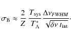 |
(7) |
In this equation, we use our observed line intensities
Table 9:
Expected values of
![]() for all six
for all six
![]() (1-0)
transitions in L1498 at the offset (60,-40) for an hour of integration and
a spectral resolution equal to 40 kHz.
(1-0)
transitions in L1498 at the offset (60,-40) for an hour of integration and
a spectral resolution equal to 40 kHz.
One sees also that without a considerable improvement in system temperature,
it will be difficult to get below
![]() limits of 200
limits of 200 ![]() G.
There have been claims of fields of this order however (e.g. Shinnaga et al. 1999); Crutcher (1999)
found a reasonable fit to the Zeeman data available at the time
of
G.
There have been claims of fields of this order however (e.g. Shinnaga et al. 1999); Crutcher (1999)
found a reasonable fit to the Zeeman data available at the time
of
![]() G
with
n4=10-4 n(H2) which would suggest that fields of
order 200
G
with
n4=10-4 n(H2) which would suggest that fields of
order 200 ![]() G are reasonable in sources like L1498. We conclude
therefore that fields of this order may be detectable using
G are reasonable in sources like L1498. We conclude
therefore that fields of this order may be detectable using
![]() but it
is extremely difficult with current sensitivities. On the other
hand, in more general, prospects do not seem worse than with CN.
but it
is extremely difficult with current sensitivities. On the other
hand, in more general, prospects do not seem worse than with CN.
8 Conclusions
We have carried out a study of the behaviour of the abundance of- 1.
- In L1498,
 shows a distribution similar to that observed
in other species attributed to depletion onto grain surfaces in the
central region; by contrast, in CB246 the dust and the
emission
have similar distributions.
shows a distribution similar to that observed
in other species attributed to depletion onto grain surfaces in the
central region; by contrast, in CB246 the dust and the
emission
have similar distributions.
- 2.
- The two cores show a clear signature for deviations from LTE
populations in
:
spectra in most positions deviate from expectations assuming LTE and thus
a single-temperature LTE model cannot fit the data.
- 3.
- There are positions of high
optical depth in both
sources; in addition, L1498 shows
self-absorption toward the dust peak.
- 4.
- Our Monte
Carlo model shows that the observed deviations from LTE
can be qualitatively
understood, but reliable collisional rate calculations for
are needed in order to make further progress.
- 5.
- The non-LTE deviations have not prevented from
computing column density values based on LTE. We also found that the
abundance relative to H2 is remarkably constant outside regions of
high CO depletion with a value of
 in L1498
and
in L1498
and
 in CB246.
One possible implication is that the abundances of
atomic oxygen and nitrogen are extremely low (below
in CB246.
One possible implication is that the abundances of
atomic oxygen and nitrogen are extremely low (below
 relative to H).
- 6.
- We derived a new set of frequencies for all the six hyperfine
components of
(1-0) and seven components of
(2-1), computing
an improved set of spectroscopic constants for
.
Acknowledgements
This effort/activity is supported by the European Community Framework Programme 7, Advanced Radio Astronomy in Europe, grant agreement No.: 227290. M.P. and D.G. acknowledge support from the EC Research Training Network MRTN-CT-2006-035890 ``Constellation: The Origin of Stellar Masses''. H.S.P.M. is grateful for support by the Bundesministerium für Bildung und Forschung (BMBF) administered through Deutsches Zentrum für Luft- und Raumfahrt (DLR). His support is aimed in particular at maintaining the CDMS.
References
- Aikawa, Y., Ohashi, N., & Herbst, E. 2003, ApJ, 593, 906 [NASA ADS] [CrossRef] (In the text)
- Aikawa, Y., Herbst, E., Roberts, H., & Caselli, P. 2005, ApJ, 620, 330 [NASA ADS] [CrossRef] (In the text)
- Akyilmaz, M., Flower, D. R., Hily-Blant, P., Pineau Des Forêts, G., & Walmsley, C. M. 2007, A&A, 462, 221 [NASA ADS] [CrossRef] [EDP Sciences] (In the text)
- André, P., Ward-Thompson, D., & Motte, F. 1996, A&A, 314, 625 [NASA ADS]
- Bel, N., & Leroy, B. 1998, A&A, 335, 1025 [NASA ADS] (In the text)
- Bergin, E. A., & Tafalla, M. 2007, Ann. Rev. A&A, 45, 339 [NASA ADS] [CrossRef] (In the text)
- Caselli, P., Myers, P. C., & Thaddeus, P. 1995, ApJ, 455, L77 [NASA ADS] [CrossRef] (In the text)
- Caselli, P., Benson, P. J., Myers, P. C., & Tafalla, M. 2002, ApJ, 572, 238 [NASA ADS] [CrossRef] (In the text)
- Chandrasekhar, S., & Münch, G. 1950, ApJ, 111, 142 [NASA ADS] [CrossRef] (In the text)
- Clemens, D. P., & Barvainis, R. 1988, ApJS, 68, 257 [NASA ADS] [CrossRef]
- Codella, C., & Scappini, F. 1998, MNRAS, 298, 1092 [NASA ADS] [CrossRef] (In the text)
- Crutcher, R. M. 1999, ApJ, 520, 706 [NASA ADS] [CrossRef] (In the text)
- Crutcher, R. M., Troland, T. H., Lazareff, B., & Kazes, I. 1996, ApJ, 456, 217 [NASA ADS] [CrossRef] (In the text)
- Dame, T. M., Ungerechts, H., Cohen, R. S., et al. 1987, ApJ, 322, 706 [NASA ADS] [CrossRef] (In the text)
- Ebenstein, W. L., & Muenter, J. S. 1984, J. Chem. Phys., 80, 3989 [NASA ADS] [CrossRef] (In the text)
- Elias, J. H. 1978, ApJ, 224, 857 [NASA ADS] [CrossRef] (In the text)
- Flower, D. R., Pineau Des Forêts, G., & Walmsley, C. M. 2006, A&A, 456, 215 [NASA ADS] [CrossRef] [EDP Sciences] (In the text)
- Falgarone, E., Troland, T. H., Crutcher, R. M., & Paubert, G. 2008, A&A, 487, 247 [NASA ADS] [CrossRef] [EDP Sciences] (In the text)
- Goodman, A. A., Benson, P. J., Fuller, G. A., & Myers, P. C. 1993, ApJ, 406, 528 [NASA ADS] [CrossRef] (In the text)
- Gottlieb, C. A., Gottlieb, E. W., & Thaddeus, P. 1983, ApJ, 264, 740 [NASA ADS] [CrossRef] (In the text)
- Green, S., & Thaddeus, P. 1974, ApJ, 191, 653 [NASA ADS] [CrossRef] (In the text)
- Guilloteau, S., & Baudry, A. 1981, A&A, 97, 213 [NASA ADS] (In the text)
- Hily-Blant, P., Walmsley, C. M., Pineau des Forêts, G., & Flower, D. 2008, A&A, 480, L5 [NASA ADS] [CrossRef] [EDP Sciences] (In the text)
- Hollenbach, D., Kaufman, M. J., Bergin, E. A., & Melnick, G. J. 2009, ApJ, 690, 1497 [NASA ADS] [CrossRef] (In the text)
- Kirk, J. M., Ward-Thompson, D., & Crutcher, R. M. 2006, MNRAS, 369, 1445 [NASA ADS] [CrossRef] (In the text)
- Launhardt, R., & Henning, T. 1997, A&A, 326, 329 [NASA ADS] (In the text)
- Lee, J.-E., Bergin, E. A., & Evans, N. J. II 2004, ApJ, 617, 360 [NASA ADS] [CrossRef] (In the text)
- Lemme, C., Wilson, T. L., Tieftrunk, A. R., & Henkel, C. 1996, A&A, 312, 585 [NASA ADS] (In the text)
- Lique, F., van der Tak, F. F. S., Kos, J., Bulthuis, J., & Alexander, M. H. 2009, A&A, 493, 557 [NASA ADS] [CrossRef] [EDP Sciences] (In the text)
- Monteiro, T. S., & Stutzki, J. 1986, MNRAS, 221, P33 [NASA ADS] (In the text)
- Müller, H. S. P., Klaus, T., & Winnewisser, G. 2000, A&A, 357, L65 [NASA ADS] (In the text)
- Müller, H. S. P., Thorwirth, S., Roth, D. A., & Winnewisser, G. 2001, A&A, 370, L49 [NASA ADS] [CrossRef] [EDP Sciences] (In the text)
- Müller, H. S. P., Schlöder, F., Stutzki, J., & Winnewisser, G. 2005, J. Mol. Struct., 742, 215 [NASA ADS] [CrossRef] (In the text)
- Myers, P. C., & Benson, P. J. 1983, ApJ, 266, 309 [NASA ADS] [CrossRef]
- Myers, P. C., Mardones, D., Tafalla, M., Williams, J. P., & Wilner, D. J. 1996, ApJ, 465, L133 [NASA ADS] [CrossRef] (In the text)
- Ohashi, N. 1999, in Proceedings of Star Formation, ed. T. Nakamoto (Nobeyama Radio Observatory), 129 (In the text)
- Pagani, L., Bacmann, A., Cabrit, S., & Vastel, C. 2007, A&A, 467, 179 [NASA ADS] [CrossRef] [EDP Sciences] (In the text)
- Pagani, L., Daniel, F., & Dubernet, M.-L. 2009, A&A, 494, 719 [NASA ADS] [CrossRef] [EDP Sciences] (In the text)
- Preibisch, Th., Ossenkopf, V., Yorke, H. W., & Henning, Th. 1993, A&A, 279, 577 [NASA ADS] (In the text)
- Sastry, K. V. L. N., Helminger, P., Charo, A., Herbst, E., & De Lucia, F. C. 1981, ApJ, 251, L119 [NASA ADS] [CrossRef] (In the text)
- Schmid-Burgk, J., Muders, D., Müller, H. S. P., & Brupbacher-Gatehouse, B. 2004, A&A, 419, 949 [NASA ADS] [CrossRef] [EDP Sciences] (In the text)
- Shinnaga, H., Tsuboi, M., & Kasuga, T. 1999, in Proceedings of Star Formation 1999, ed. T. Nakamoto (Nobeyama Radio Observatory), 175 (In the text)
- Shirley, Y. L., Nordhaus, M. K., Grcevich, J. M., et al. 2005, ApJ, 632, 982 [NASA ADS] [CrossRef]
- Tafalla, M., Myers, P. C., Caselli, P., Walmsley, C. M., & Comito, C. 2002, ApJ, 569, 815 [NASA ADS] [CrossRef] (In the text)
- Tafalla, M., Myers, P. C., Caselli, P., & Walmsley, C. M. 2004, A&A, 416, 191 [NASA ADS] [CrossRef] [EDP Sciences] (In the text)
- Tafalla, M., Santiago-García, J., Myers, P. C., et al. 2006, A&A, 455, 577 [NASA ADS] [CrossRef] [EDP Sciences] (In the text)
- Tassoul, J.-L. 1978, Theory of Rotating Stars (Princeton: Princeton Univ. Press) (In the text)
- Terzieva, R., & Herbst, E. 1998, ApJ, 501, 207 [NASA ADS] [CrossRef] (In the text)
- Thum, C., Wiesemeyer, H., Paubert, G., Navarro, S., & Morris, D. 2008, PASP, 120, 777 [NASA ADS] [CrossRef]
- Turner, B. E., Terzieva, R., & Herbst, E. 1999, ApJ, 518, 699 [NASA ADS] [CrossRef] (In the text)
- Walmsley, C. M., Flower, D. R., & Pineau des Forêts, G. 2004, A&A, 418, 1035 [NASA ADS] [CrossRef] [EDP Sciences] (In the text)
- Woodall, J., Agúndez, M., Markwick-Kemper, A. J., & Millar, T. J. 2007, A&A, 46, 1197 [NASA ADS] [CrossRef] (In the text)
Footnotes
All Tables
Table 1:
Line parametersa observed in
![]() (1-0)
(1-0)
Table 2:
Line parametersa observed in
![]() (2-1).
(2-1).
Table 3: Results of gradient fitting.
Table 4:
Observed hyperfine structure components of the
![]() transition in
transition in
![]() :
rest frequenciesa, residuals
:
rest frequenciesa, residuals ![]() between observed and calculated frequenciesb,
and relative intensities f.
between observed and calculated frequenciesb,
and relative intensities f.
Table 5:
Observed hyperfine structure components of the
![]() transition
in
transition
in
![]() :
rest frequenciesa, residuals
:
rest frequenciesa, residuals ![]() between observed and calculated frequenciesb,
and relative intensities f.
between observed and calculated frequenciesb,
and relative intensities f.
Table 6: Spectroscopic parametersa (MHz) of C2H in comparison to previous values.
Table 7:
Values of
![]() [K] derived using the two
methods.
[K] derived using the two
methods.
Table 8: Molecular abundances in L1498 and CB246.
Table 9:
Expected values of
![]() for all six
for all six
![]() (1-0)
transitions in L1498 at the offset (60,-40) for an hour of integration and
a spectral resolution equal to 40 kHz.
(1-0)
transitions in L1498 at the offset (60,-40) for an hour of integration and
a spectral resolution equal to 40 kHz.
All Figures
| |
Figure 1:
Dust emission at 1.3 mm (after smoothing to 28
|
| Open with DEXTER | |
| In the text | |
| |
Figure 2:
Upper panel: dust emission at 1.3 mm (after smoothing to
28
|
| Open with DEXTER | |
| In the text | |
| |
Figure 3:
Upper panels: continuum emission flux measured along the
NW-SE
cut in L1498,
see Fig. 1, and along the EW cut of the SE peak
in CB246,
see upper panel of Fig. 2.
Lower panels: ratio between the integrated intensity of the different
hyperfine components
of
|
| Open with DEXTER | |
| In the text | |
| |
Figure 4:
Component 2 ( black), 3 ( green), 4 ( blue) and 5 ( red) of
|
| Open with DEXTER | |
| In the text | |
| |
Figure 5:
Hyperfine components of
|
| Open with DEXTER | |
| In the text | |
| |
Figure 6:
Upper panels: continuum emission flux measured along the SN cut of the SE
and the NW peaks in CB246, see upper panel of Fig. 2.
Lower panels: ratio between the integrated intensity of the component 2 of
|
| Open with DEXTER | |
| In the text | |
| |
Figure 7:
Radial profile of line center velocity for L1498 ( upper panel)
and CB246 ( lower panel) derived from the hyperfine-structure fits of
|
| Open with DEXTER | |
| In the text | |
| |
Figure 8:
|
| Open with DEXTER | |
| In the text | |
| |
Figure 9:
Ratio of the integrated intensities of some couples of components of
|
| Open with DEXTER | |
| In the text | |
| |
Figure 10:
Ratio of the integrated intensities of some couples of components of
|
| Open with DEXTER | |
| In the text | |
| |
Figure 11: Comparison between observations and our best fit Monte Carlo model of the C2H emission in L1498. Top panel: radial profile of observed C2H(1-0) intensity integrated over all hyperfine components ( filled squares) and model prediction for a constant abundance core with a central depletion hole ( solid red line). Middle panels: emerging spectra for each component of the C2H(1-0) multiplet ( black histograms) and predictions for the same best fit model ( solid red lines). Bottom panels: same as middle panels but for the components of the C2H(2-1) multiplet. Note the reasonably good fit of all observables despite the use of highly approximated collisional rates (see text). |
| Open with DEXTER | |
| In the text | |
| |
Figure 12: Radial profile of excitation temperature for each hyperfine component of C2H(1-0) as predicted by our best fit Monte Carlo model (each component is labelled according to the ordering in Table 3). Note the gradual drop of Tex with radius, which is caused by the combined decrease in collisional excitation and photon trapping towards the outer core. The different hyperfine components have different Tex depending mostly on trapping effects (see text for a full discussion). |
| Open with DEXTER | |
| In the text | |
| |
Figure 13:
Plot of the column density of
|
| Open with DEXTER | |
| In the text | |
Copyright ESO 2009
Current usage metrics show cumulative count of Article Views (full-text article views including HTML views, PDF and ePub downloads, according to the available data) and Abstracts Views on Vision4Press platform.
Data correspond to usage on the plateform after 2015. The current usage metrics is available 48-96 hours after online publication and is updated daily on week days.
Initial download of the metrics may take a while.