| Issue |
A&A
Volume 505, Number 3, October III 2009
|
|
|---|---|---|
| Page(s) | 1213 - 1219 | |
| Section | Stellar structure and evolution | |
| DOI | https://doi.org/10.1051/0004-6361/200811612 | |
| Published online | 11 August 2009 | |
On the afterglow from the receding jet of  -ray bursts
X. Wang - Y. F. Huang - S. W. Kong
Department of Astronomy, Nanjing University, Nanjing 210093, PR China
Received 31 December 2008 / Accepted 29 June 2009
Abstract
According to popular progenitor models of gamma-ray bursts, twin
jets should be launched by the central engine, with a forward jet
moving toward the observer and a receding jet (or the counter jet)
moving backwardly. However, in calculating the afterglows, usually
only the emission from the forward jet is considered. Here we
present a detailed numerical study on the afterglow from the
receding jet. Our calculation is based on a generic dynamical
description, and includes some delicate ingredients such as the
effect of the equal arrival time surface. It is found that the
emission from the receding jet is generally rather weak. In radio
bands, it usually peaks at a time
![]() d, with the peak
flux nearly 4 orders of magnitude lower than the peak flux of the
forward jet. Also, it usually manifests as a short plateau in the
total afterglow light curve, but not as an obvious rebrightening as
once expected. In optical bands, the contribution from the receding
jet is even weaker, with the peak flux being
d, with the peak
flux nearly 4 orders of magnitude lower than the peak flux of the
forward jet. Also, it usually manifests as a short plateau in the
total afterglow light curve, but not as an obvious rebrightening as
once expected. In optical bands, the contribution from the receding
jet is even weaker, with the peak flux being ![]() 23 mag
lower than the peak flux of the forward jet. We thus argue that the
emission from the receding jet is very difficult to detect. However,
in some special cases, i.e., when the circum-burst medium density is
very high, or if the parameters of the receding jet are quite
different from those of the forward jet, the emission from the
receding jet can be significantly enhanced and may still emerge as a
marked rebrightening. We suggest that the search for receding jet
emission should mostly concentrate on nearby gamma-ray bursts, and
the observation campaign should last for at least several hundred
days for each event.
23 mag
lower than the peak flux of the forward jet. We thus argue that the
emission from the receding jet is very difficult to detect. However,
in some special cases, i.e., when the circum-burst medium density is
very high, or if the parameters of the receding jet are quite
different from those of the forward jet, the emission from the
receding jet can be significantly enhanced and may still emerge as a
marked rebrightening. We suggest that the search for receding jet
emission should mostly concentrate on nearby gamma-ray bursts, and
the observation campaign should last for at least several hundred
days for each event.
Key words: gamma rays: bursts - ISM: jets and outflows - stars: neutron
1 Introduction
Thanks to the discovery of X-ray, optical and radio afterglows of gamma-ray bursts (GRBs), it is now clear that most GRBs are situated at cosmological distances (Costa et al. 1997; van Paradijs et al. 1997; Frail et al. 1997). Much progress has been achieved during the past decade (Piran 2004; Mészáros 2006). Especially, through the detection of GRB 030329, the association of long GRBs with supernovae is firmly established (Hjorth et al. 2003), which strongly supports the collapsar model as the energy mechanism for long GRBs (Woosley 1993; MacFadyen & Woosley 1999). Theoretically, the collapse of a massive star will most likely give birth to a black hole, surrounded by a temporal accretion disk. It is logical that the accretion system will produce double-sided jets (MacFadyen & Woosley 1999; Aloy et al. 2000; Rhoads 1999; Mészáros 2002). The GRB can be observed only when our line of sight lies on one of the two jets. The collimation of GRB ejecta can be tested observationally, through various beaming effects, such as the achromatic break in GRB afterglow light curves (Sari et al. 1999; Liang et al. 2008), the polarization in both the main burst phase and the afterglow phase (Lazzati 2006), the predicted existence of orphan afterglows (Rhoads 1997; Huang et al. 2002; Granot & Loeb 2003), and the ``energy crisis'' already noted in some GRBs (Frail et al. 2001). In fact, more and more observational evidence has been accumulated supporting the idea that many GRB ejecta might be highly collimated.
Current studies on beaming effects are mostly concentrated on the emission from the forward jet, i.e., the jet moving toward the observer. The emission from the receding jet (or the counter jet) is generally omitted. It is interesting to note that this ingredient recently has been studied by a few authors (Granot & Loeb 2003; Li & Song 2004). By some simple analytical derivations, Li & Song (2004) argued that the emission from the receding jet can be detected in a few cases in the non-relativistic phase of GRB afterglows. However, previous studies did not consider some important effects, such as the action of the equal arrival time surface (EATS). Recently, Zhang & MacFadyen (2009) presented a two-dimensional simulation of GRB outflow. The emission from the receding jet was included in their calculations, but they did not investigate the effects of various parameters on the receding jet component.
In this paper, we will present our detailed numerical investigation of the emission from the receding jet of GRBs in the deep Newtonian stage. Although the GRB jet may be complicatedly structured (Mészáros et al. 1998; Kumar & Granot 2003; Huang et al. 2004), and the circum-burst environment may be a wind medium and even associated with some complex density variations (Mészáros et al. 1998; Chevalier & Li 2000; Gou et al. 2001; Wu et al. 2004), here we will only consider the simplest situation, i.e, the homogeneous double-sided jets expanding into a homogeneous interstellar medium, which is favored by some recent fits (Huang et al. 2000a; Yost et al. 2003).
The structure of our paper is as follows. Section 2 is a review of the dynamics and radiation model we used in our calculations. In Sect. 3 we present the numerical results, together with our explanations. Section 4 is our conclusion and discussion.
2 Model description
In the afterglow phase, the GRB ejecta expand into the interstellar medium (ISM) and are decelerated continuously, giving rise to a strong external shock. The swept-up electrons are accelerated by the blastwave, producing the afterglow mainly through synchrotron radiation. In radio bands, the shell is no longer optically thin, so that the synchrotron self-absorption should be considered. In our study, we will use the simplified dynamical equations suggested by Huang et al. (1999, 2000b), which are consistent with the self-similar solution of Blandford & McKee (1976) in the ultra-relativistic phase, and consistent with the Sedov solution (Sedov 1969) in the non-relativistic phase. The beaming effects (Rhoads 1997, 1999) can also be conveniently simulated in this way. Here, for completeness, we first describe the dynamics and the radiation process.
2.1 Hydrodynamic evolution
In our description, t is the photon arrival time measured in the
lab frame; R is the radial coordinate measured in the burst frame
relative to the initiation point; m is the rest mass of the
swept-up medium; ![]() is the half-opening angle of the ejecta;
is the half-opening angle of the ejecta;
![]() is the bulk Lorentz factor of the moving material; p is
the electron distribution index which is typically between 2 and 3;
n is the number density of ISM;
is the bulk Lorentz factor of the moving material; p is
the electron distribution index which is typically between 2 and 3;
n is the number density of ISM;
![]() and
and
![]() are the energy equipartition factors for electrons and the comoving
magnetic field. We further denote the initial values of the rest
mass, the isotropic equivalent energy, the Lorentz factor and the
half-opening angle of the ejecta as
are the energy equipartition factors for electrons and the comoving
magnetic field. We further denote the initial values of the rest
mass, the isotropic equivalent energy, the Lorentz factor and the
half-opening angle of the ejecta as
![]() ,
respectively.
,
respectively.
The overall dynamical evolution of the GRB ejecta can be depicted by
| |
= |  |
(1) |
| = | (2) | ||
| = |  |
(3) | |
| = |  |
(4) |
where
Equations (1)-(4) is a convenient description of GRB afterglow dynamics that is applicable in both the initial ultra-relativistic phase and the late Newtonian phase.
2.2 Radiation process
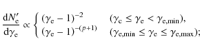
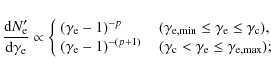
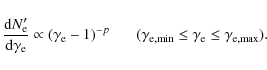
We assume that the shock-accelerated electrons follow a power-law
distribution according to their energies,
![]() ,
However, to ensure that the calculation in the deep Newtonian phase is correct, we
need to modify the basic distribution function as
,
However, to ensure that the calculation in the deep Newtonian phase is correct, we
need to modify the basic distribution function as
![]() (Huang & Cheng 2003). The minimum and maximum Lorentz factors of
electrons can be calculated as
(Huang & Cheng 2003). The minimum and maximum Lorentz factors of
electrons can be calculated as
![]() and
and
![]() ,
where B' is the comoving
magnetic field strength,
,
where B' is the comoving
magnetic field strength, ![]() and
and ![]() are masses of
the proton and electron, respectively. As usual, we assume that the
energy ratio of the magnetic field with respect to internal energy
is
are masses of
the proton and electron, respectively. As usual, we assume that the
energy ratio of the magnetic field with respect to internal energy
is
![]() ,
so that the energy density of the magnetic field
is
,
so that the energy density of the magnetic field
is
![]() .
.
The cooling of electrons due to synchrotron radiation will lead to a
steep distribution function above a critical Lorentz factor,
![]() .
The expression for
.
The expression for
![]() can be derived
as
can be derived
as
![]() ,
where
,
where
![]() is the Thompson scattering
cross section (Sari et al. 1998). Considering all the above
ingredients, we finally use the following electron distribution
function in our calculations (Huang & Cheng 2003):
is the Thompson scattering
cross section (Sari et al. 1998). Considering all the above
ingredients, we finally use the following electron distribution
function in our calculations (Huang & Cheng 2003):
1.
![]() ,
,
 |
(5) |
2.
![]() ,
,
 |
(6) |
3.
![]() ,
,
 |
(7) |
In the comoving frame, the synchrotron radiation power at
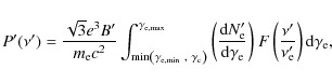 |
(8) |
with
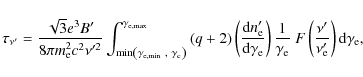 |
(9) |
where
 |
(10) |
Let us define the Doppler-factor as
![\begin{displaymath}F_\nu = \frac{(1 + z) D^3 }{4\pi d_{\rm L}^2 } f(\tau) P'\left[ (1 +
z)D^{-1} \nu \right],
\end{displaymath}](/articles/aa/full_html/2009/39/aa11612-08/img59.png) |
(11) |
where
 |
(12) |
3 Numerical results
In this section, we present our numerical results concerning the
emission from the receding jet. For simplicity, we assume that the
twin jets have the same characteristics, i.e., the same initial
energy, opening angle, initial Lorentz factor, and the circum-burst
ISM density. We also assume that the microphysics shock parameters
(p,
![]() ,
,
![]() )
are the same for the receding
and forward blastwaves. For convenience, we define a set of
parameter values as the ``standard'' condition:
)
are the same for the receding
and forward blastwaves. For convenience, we define a set of
parameter values as the ``standard'' condition:
![]() ,
,
![]() ,
,
![]() ,
,
![]() ,
,
![]() ,
,
![]() ,
p=2.5,
,
p=2.5,
![]() ,
and
,
and
![]() .
These values
are typical in the study of GRB afterglows. For redshift, we adopt
the value of z=0.1 (which corresponds to
.
These values
are typical in the study of GRB afterglows. For redshift, we adopt
the value of z=0.1 (which corresponds to
![]() Mpc
according to the popular cosmology model, Wright 2006).
Mpc
according to the popular cosmology model, Wright 2006).
![\begin{figure}
\par\includegraphics[width=9cm,clip]{11612f1.eps}
\end{figure}](/articles/aa/full_html/2009/39/aa11612-08/img70.png) |
Figure 1: The evolution of the Lorentz factors of the twin jets. The solid line corresponds to the receding jet and the dashed line is plotted for the forward jet. The twin jets are in the ``standard'' condition as defined in Sect. 3. The observers' time has been corrected for the cosmological effect (z=0.1). |
| Open with DEXTER | |
We illustrate the evolution of the Lorentz factors of the twin jets
in Fig. 1. Note that the X-axis is observers' time. For the
observer, the dynamical evolution of the receding jet is quite
different from that of the forward jet, especially in the
relativistic phase. We see that for a rather long time (![]() d),
d), ![]() of the receding jet remains almost constant. This is
due to the time delay induced by the long distance between the twin
jets. It also implies that the emission from the receding jet will
be very weak in this period, since it is highly beamed backward. At
the observers' time of
of the receding jet remains almost constant. This is
due to the time delay induced by the long distance between the twin
jets. It also implies that the emission from the receding jet will
be very weak in this period, since it is highly beamed backward. At
the observers' time of
![]() d, the Lorentz factor of the
receding jet is still more than 10, while the forward jet's Lorentz
factor has already decreased to less than 1.1.
d, the Lorentz factor of the
receding jet is still more than 10, while the forward jet's Lorentz
factor has already decreased to less than 1.1.
![\begin{figure}
\par\includegraphics[width=9cm,clip]{11612f2.eps}
\end{figure}](/articles/aa/full_html/2009/39/aa11612-08/img73.png) |
Figure 2:
Schematic illustration of the EATSs at three
moments,
|
| Open with DEXTER | |
In Fig. 2, we show some examples of the equal arrival time surfaces (EATSs) at three moments. As expected, at any particular moment, the typical radius of the surface is much larger for the forward jet branch compared to that for the receding jet branch. Also, we notice that the curvature of the two branches is quite different. Generally, the EATS is much flatter on the receding jet. Another interesting feature is that the area of the EATS on the forward branch is much larger than that of the corresponding receding branch.
![\begin{figure}
\par\includegraphics[width=7cm,clip]{11612f3a.eps}\hspace*{1cm}
\includegraphics[width=7cm,clip]{11612f3b.eps}
\end{figure}](/articles/aa/full_html/2009/39/aa11612-08/img74.png) |
Figure 3:
8.46 GHz radio afterglow a) and R-band optical afterglow b) from
the forward jet and the receding jet. The thick lines are plotted
for a ``standard'' double-sided jet as defined in Sect. 3. The thin lines are plotted
for the double-sided jet with only one parameter altered compared to the ``standard''
condition, i.e.
|
| Open with DEXTER | |
Figure 3 shows the radio and optical afterglow light curves under the ``standard'' condition (thick lines). Here, the thick dotted line corresponds to emission from the forward jet, the thick dashed line corresponds to emission from the receding jet, and the thick sold line is the total light curve. Under the ``standard'' condition, for the forward jet, the afterglow light curve (the dotted line) becomes slightly flattened in the non-relativistic phase. It is consistent with previous results in the deep Newtonian phase (Huang & Cheng 2003). Also it can be seen that the receding jet really can contribute a significant portion in the total emission at very late stage. The role played by the receding jet is reasonably more important in the radio band than in the optical band. However, the dashed component is generally not very strong, so that it can only lead to a plateau in the total light curve, but not an obvious rebrightening or a marked peak as expected by Li & Song (2004). Interestingly, our result is consistent with the simulation of Zhang & Macfadyen (2009). We believe that the discrepancy between our numerical result and Li & Song's analytical result mainly comes from the effect of the EATS. Below, we will give some detailed analyses on this point. Additionally, it should be noted that in the radio band, the peak flux of the receding component is about 4 orders of magnitude weaker than that of the forward component. It essentially means that the receding component is very weak, and is very difficult to detect. In the optical band, the condition is even more awkward. The peak flux of the receding component is about 23 mag dimmer than that of the forward component in R band. Even comparing with the flux of the forward jet at the jet break time, it is still 16-17 mag weaker. So, in the optical band, it is even much more difficult to observe the receding jet component.
According to Li & Song (2004), the time when the receding jet
becomes notably visible (
![]() )
is relevant to the
time when the forward jet enters the non-relativistic phase (
)
is relevant to the
time when the forward jet enters the non-relativistic phase (
![]() ), i.e.,
), i.e.,
 |
(13) |
where
 |
(14) |
Adopting the standard values of our parameters, Eq. (14) yields
Another reason that suppresses the rebrightening of the receding jet
is as follows. According to Li & Song's analysis, at the observers'
time t3, the receding jet should be at the radius of
![]() .
However, from our Fig. 2, we see that the typical radius of
the EATS at t3 on the receding jet is much smaller than the
radius of the forward jet at t1. The reason is again due to the
EATS effect. This means that the receding jet still does not
decelerate enough at t3 (actually, the bulk Lorentz factor is
still 3.95), and its emission is still mainly directed forward (not
backward toward the observer). Additionally, Fig. 2 shows clearly
that the area of the receding jet at t3 (corresponding to
.
However, from our Fig. 2, we see that the typical radius of
the EATS at t3 on the receding jet is much smaller than the
radius of the forward jet at t1. The reason is again due to the
EATS effect. This means that the receding jet still does not
decelerate enough at t3 (actually, the bulk Lorentz factor is
still 3.95), and its emission is still mainly directed forward (not
backward toward the observer). Additionally, Fig. 2 shows clearly
that the area of the receding jet at t3 (corresponding to
![]() )
is much smaller than that of the forward jet at
t1 (corresponding to
)
is much smaller than that of the forward jet at
t1 (corresponding to
![]() ). So, the number of electrons
involved in the radiation process is typically much smaller in the
receding jet at
). So, the number of electrons
involved in the radiation process is typically much smaller in the
receding jet at
![]() ,
compared to that in the
forward jet at
,
compared to that in the
forward jet at
![]() .
Due to the above reasons, the
contribution from the receding jet is naturally much weaker than
that deduced from
.
Due to the above reasons, the
contribution from the receding jet is naturally much weaker than
that deduced from
![]() (Eq. (7) in
Li & Song 2004).
(Eq. (7) in
Li & Song 2004).
However, although the receding jet emission is generally very weak
in our ``standard'' condition, we hypothesize that in some special
cases it still can be enhanced. Obviously, a denser environment will
help to decelerate the jet more quickly, thus lead to a smaller
![]() and a higher intensity.
In Fig. 3, we have also plotted in thin lines our numerical results
for a double-sided jet located in a dense circum-burst medium
(
and a higher intensity.
In Fig. 3, we have also plotted in thin lines our numerical results
for a double-sided jet located in a dense circum-burst medium
(
![]() ).
Note that other parameters involved here are the same as the
``standard'' case. Encouragingly, in Fig. 3a we see that the peak
time of the receding jet can be as early as
).
Note that other parameters involved here are the same as the
``standard'' case. Encouragingly, in Fig. 3a we see that the peak
time of the receding jet can be as early as
![]() d, with the peak flux as large as a few mJy in radio band (i.e.,
only several times less than the peak level of the forward jet). In
Fig. 3b, the optical contribution from the receding jet is still
very weak, with the peak flux being about 28
d, with the peak flux as large as a few mJy in radio band (i.e.,
only several times less than the peak level of the forward jet). In
Fig. 3b, the optical contribution from the receding jet is still
very weak, with the peak flux being about 28![]() .
.
![\begin{figure}
\par\includegraphics[width=7.2cm,clip]{11612f4a.eps}\hspace*{0.8cm}
\includegraphics[width=7cm,clip]{11612f4b.eps}
\end{figure}](/articles/aa/full_html/2009/39/aa11612-08/img94.png) |
Figure 4: Multiwavelength afterglow light curves of a double-sided jet. Radio afterglows are illustrated in panel a), and optical/IR afterglows are plotted in panel b). In this calculation, we have used the ``standard'' parameter set as defined in Sect. 3. |
| Open with DEXTER | |
![\begin{figure}
\par\includegraphics[width=6.7cm,clip]{11612f5a.eps}\hspace*{1cm}...
...s}\hspace*{1cm}
\includegraphics[width=6.7cm,clip]{11612f5d.eps}
\end{figure}](/articles/aa/full_html/2009/39/aa11612-08/img95.png) |
Figure 5:
The effects of various parameters (n,
|
| Open with DEXTER | |
Figure 5 illustrates the effects of some parameters (n,
![]() ,
,
![]() ,
and
,
and
![]() )
on the receding jet
component in the afterglow light curve. Figure 5a shows that the
circum-burst medium density (n) affects the peak time (
)
on the receding jet
component in the afterglow light curve. Figure 5a shows that the
circum-burst medium density (n) affects the peak time (
![]() )
of receding jet dramatically. A higher number density
usually leads to a smaller
)
of receding jet dramatically. A higher number density
usually leads to a smaller
![]() .
The strength of the
receding jet component is also obviously enhanced.
It again hints that the receding jet component is most likely
detectable in a dense environment. Similarly, the initial kinetic
energy (
.
The strength of the
receding jet component is also obviously enhanced.
It again hints that the receding jet component is most likely
detectable in a dense environment. Similarly, the initial kinetic
energy (
![]() )
also affects
)
also affects
![]() significantly,
with larger
significantly,
with larger
![]() corresponding to a larger
corresponding to a larger
![]() (Fig. 5b). The effect of the initial jet opening angle
(
(Fig. 5b). The effect of the initial jet opening angle
(
![]() )
on
)
on
![]() can also be clearly seen in
Fig. 5c. It should be further noted that the receding jet
component is more marked when the opening angle is smaller. In
Fig. 5d, we can observe an obvious rebrightening when the
radiation efficiency (
can also be clearly seen in
Fig. 5c. It should be further noted that the receding jet
component is more marked when the opening angle is smaller. In
Fig. 5d, we can observe an obvious rebrightening when the
radiation efficiency (
![]() )
is large. However, in a
realistic case,
)
is large. However, in a
realistic case,
![]() is unlikely to be so large. At such
late stages, the external shock should be adiabatic, so that
is unlikely to be so large. At such
late stages, the external shock should be adiabatic, so that
![]() should be nearly zero.
should be nearly zero.
![\begin{figure}
\par\includegraphics[width=6.7cm,clip]{11612f6a.eps}\hspace*{0.8c...
...\hspace*{0.8cm}
\includegraphics[width=6.7cm,clip]{11612f6d.eps}
\end{figure}](/articles/aa/full_html/2009/39/aa11612-08/img96.png) |
Figure 6:
The effects of various parameters (
|
| Open with DEXTER | |
In Fig. 5d, we also plot the radio afterglow light curves for
double-sided jets under some special physical assumptions. The
dash-dotted line is plotted by assuming that both the forward jet
and the receding jet do not experience any lateral expansion. Since
the deceleration of the jets is much slower in this case, we see
that the receding jet component emerges much later and is also much
less obvious compared to our ``standard'' case. The dotted line is
plotted by assuming a much smaller initial Lorentz factor (
![]() ), which may correspond to the so-called failed GRBs (Huang et al. 2002). The receding jet component emerges slightly earlier
compared to the solid line, but its role becomes correspondingly
less significant.
), which may correspond to the so-called failed GRBs (Huang et al. 2002). The receding jet component emerges slightly earlier
compared to the solid line, but its role becomes correspondingly
less significant.
Figure 6 illustrates the effects of the other four parameters
(
![]() ,
,
![]() ,
p, and
,
p, and
![]() )
on the
receding jet component. Generally speaking, a larger
)
on the
receding jet component. Generally speaking, a larger
![]() and/or
and/or
![]() can enhance the receding jet component
markedly. On the other hand, although p has an important influence
on the overall afterglow light curve, its impact on the relative
strength of the receding jet component is not significant. Again,
note that in all the cases, the contribution from the receding jet
only emerges as a plateau, but not as any obvious rebrightening. In
Fig. 6d, when the observing angle (
can enhance the receding jet component
markedly. On the other hand, although p has an important influence
on the overall afterglow light curve, its impact on the relative
strength of the receding jet component is not significant. Again,
note that in all the cases, the contribution from the receding jet
only emerges as a plateau, but not as any obvious rebrightening. In
Fig. 6d, when the observing angle (
![]() )
increases,
the forward jet component becomes weaker, while the receding jet
component becomes stronger. It is in accord with our expectation
(also see Granot & Loeb 2003). However, the contribution from the
receding jet still generally plays a minor role in the total
afterglow light curve. Additionally, for off-axis twin jets, the GRB
from the forward jet is un-observable, so that even the afterglow
from the forward jet itself (i.e., the orphan afterglow) is
difficult to observe. Note that in Fig. 6d, when
)
increases,
the forward jet component becomes weaker, while the receding jet
component becomes stronger. It is in accord with our expectation
(also see Granot & Loeb 2003). However, the contribution from the
receding jet still generally plays a minor role in the total
afterglow light curve. Additionally, for off-axis twin jets, the GRB
from the forward jet is un-observable, so that even the afterglow
from the forward jet itself (i.e., the orphan afterglow) is
difficult to observe. Note that in Fig. 6d, when
![]() (i.e., the thick solid line), the contribution from the
receding jet and the forward jet are equal.
(i.e., the thick solid line), the contribution from the
receding jet and the forward jet are equal.
Equation (14) tells us that the peak time of the receding component
should be relevant to the 3 parameters of n,
![]() ,
,
![]() ;
on the other hand, other parameters such as
;
on the other hand, other parameters such as
![]() ,
,
![]() ,
p do not affect the peak time.
These tendencies can be clearly seen in Figs. 5 and 6.
,
p do not affect the peak time.
These tendencies can be clearly seen in Figs. 5 and 6.
![\begin{figure}
\par\includegraphics[width=6.7cm,clip]{11612f7a.eps}\hspace*{0.8c...
...\hspace*{0.8cm}
\includegraphics[width=6.7cm,clip]{11612f7d.eps}
\end{figure}](/articles/aa/full_html/2009/39/aa11612-08/img99.png) |
Figure 7:
8.46 GHz radio afterglow light curves of double-sided jets. In this figure, we
assume that the parameters of the receding jet can be different from those of the forward jet.
In each panel, the solid line is plotted under the ``standard'' condition, i.e., the parameters
are the same for the twin jets (but note that we have evaluated
|
| Open with DEXTER | |
In all the above calculations, we have assumed that the conditions
and parameters of the twin jets are the same. However, this may not
be the case for realistic GRBs. The circum-burst environment and the
micro-physics parameters may actually be different for the twin
jets, as may happen in the two component jet structure (Huang et al.
2004; Jin et al. 2007; Racusin et al. 2008). In Fig. 7, we have
plotted the overall afterglow light curves by assuming different
parameters for the forward jet and the receding jet. In each panel
of Fig. 7, we first plot a common light curve (the solid line) by
adopting the standard parameter set, but change
![]() to
0.01 and change
to
0.01 and change
![]() to 10-4. We then increase the
values of
to 10-4. We then increase the
values of
![]() ,
,
![]() ,
and n for the receding
jet to see their effects on the afterglow light curve. It is
encouraging to see that the emission from the receding jet can be
greatly enhanced, so that it can manifest as an obvious
rebrightening in the overall light curve. In Figs. 7a, b and d, the peak flux of the rebrightening can be nearly 100 times
larger than the ``background'' level in the best cases. It is
imaginable that in the most favorable cases, when all
,
and n for the receding
jet to see their effects on the afterglow light curve. It is
encouraging to see that the emission from the receding jet can be
greatly enhanced, so that it can manifest as an obvious
rebrightening in the overall light curve. In Figs. 7a, b and d, the peak flux of the rebrightening can be nearly 100 times
larger than the ``background'' level in the best cases. It is
imaginable that in the most favorable cases, when all
![]() ,
,
![]() and n are larger for the receding jet at the same
time, the rebrightening will be even more remarkable. However, note
that the contrary condition may also exist in realistic GRBs, i.e.,
these parameters may also be smaller for the receding jet. Then the
emission from the receding jet will be unnoticeable.
and n are larger for the receding jet at the same
time, the rebrightening will be even more remarkable. However, note
that the contrary condition may also exist in realistic GRBs, i.e.,
these parameters may also be smaller for the receding jet. Then the
emission from the receding jet will be unnoticeable.
4 Conclusion and discussion
We have studied the emission of the receding jet numerically. The
effect of the EATS is included in our calculations. Clearly, this
effect plays an important role in the process. It is found that the
contribution from the receding jet is generally quite weak. In most
cases, it only manifests as a short plateau in the overall afterglow
light curve, but not a marked rebrightening. The flux density of the
plateau is usually much less than 100 ![]() Jy in radio bands even at
a small redshift of z=0.1. If we place the GRB at a more typical
redshift of z=1, then the flux density of the plateau will be less
than 0.1
Jy in radio bands even at
a small redshift of z=0.1. If we place the GRB at a more typical
redshift of z=1, then the flux density of the plateau will be less
than 0.1 ![]() Jy at 8.46 GHz. We noticed that the observed radio
afterglow emission is generally on the level of 0.1-1 mJy at
about the peak time. After several months, the radio afterglow
usually decreases to a very low level, and is submerged by the
emission from the host galaxy, whose strength can be 40-70
Jy at 8.46 GHz. We noticed that the observed radio
afterglow emission is generally on the level of 0.1-1 mJy at
about the peak time. After several months, the radio afterglow
usually decreases to a very low level, and is submerged by the
emission from the host galaxy, whose strength can be 40-70 ![]() Jy (Berger et al. 2001). Additionally, the error bar of radio
observations is usually
Jy (Berger et al. 2001). Additionally, the error bar of radio
observations is usually ![]() 30-50
30-50 ![]() Jy at very late
stages (Frail et al. 2003). Thus the contribution from the receding
jet, i.e. the plateau, is actually very difficult to detect,
especially for those GRBs at
Jy at very late
stages (Frail et al. 2003). Thus the contribution from the receding
jet, i.e. the plateau, is actually very difficult to detect,
especially for those GRBs at ![]() .
Our results are consistent
with a recent observational report by van der Horst et al. (2008),
who failed to detect any clear clues of the receding jet emission.
.
Our results are consistent
with a recent observational report by van der Horst et al. (2008),
who failed to detect any clear clues of the receding jet emission.
However, as shown in our Fig. 7, if the micro-physics parameters of
the receding jet were different from the forward jet, or if the
receding jet were in a much denser environment, then it is still
possible that the contribution from the receding jet can be greatly
enhanced. For example, if
![]() and/or
and/or
![]() of
the receding jet is much larger than that of the forward jet, then
the receding jet can manifest as an obvious rebrightening.
of
the receding jet is much larger than that of the forward jet, then
the receding jet can manifest as an obvious rebrightening.
Also, our Fig. 5a shows that a dense circum-burst environment can
suppress the emission of the forward jet, and enhance the
contribution from the receding jet. If the GRB occurs in a very
dense molecular cloud with
![]() (Dai & Lu
1999), the contribution from the receding jet may be much easier to
detect. Additionally, if the GRB is very near to us at the same
time, then the possibility of successfully detecting the receding
jet is very high (see the thin lines in Fig. 3a).
(Dai & Lu
1999), the contribution from the receding jet may be much easier to
detect. Additionally, if the GRB is very near to us at the same
time, then the possibility of successfully detecting the receding
jet is very high (see the thin lines in Fig. 3a).
In short, we believe that the effort of trying to search for the
afterglow contribution from the receding jet is still meaningful. If
observed, it would provide useful clues to study the circum-burst
environment and the micro-physics of external shocks. We suggest
that nearby GRBs (with redshift
![]() )
should be good
candidates for such studies.
)
should be good
candidates for such studies.
Acknowledgements
We would like to thank the anonymous referee for constructive suggestions that lead to an overall improvement of this study. We also thank Z. Li for stimulating discussion. This research was supported by the National Natural Science Foundation of China (grant 10625313), and by the National Basic Research Program of China (grant 2009CB824800). Xin Wang is also supported by 2008' National Undergraduate Innovation Program of China (grant 081028441).
References
- Aloy, M. A., Müller, E., Ibáñez, J., Martí, J., & MacFadyen, A. 2000, ApJ, 531, L119 [NASA ADS] [CrossRef] (In the text)
- Berger, E., Kulkarni, S. R., & Frail, D. A. 2001, ApJ, 560, 652 [NASA ADS] [CrossRef] (In the text)
- Blandford, R. D., & McKee, C. F. 1976, Phys. Fluids, 19, 1130 [NASA ADS] [CrossRef] (In the text)
- Chevalier, R. A., & Li, Z. Y. 2000, ApJ, 536, 195 [NASA ADS] [CrossRef] (In the text)
- Costa, E., Frontera, F., Heise, J., et al. 1997, Nature, 387, 783 [NASA ADS] [CrossRef] (In the text)
- Dai, Z. G., & Lu, T. 1999, ApJ, 519, L155 [NASA ADS] [CrossRef]
- Frail, D. A., Kulkarni, S. R., Berger, E., & Wieringa, M. H. 2003, AJ, 125, 2299 [NASA ADS] [CrossRef] (In the text)
- Frail, D. A., Kulkarni, S. R., Nicastro, S. R., Feroci, M., & Taylor, G. B. 1997, Nature, 389, 261 [NASA ADS] [CrossRef] (In the text)
- Frail, D. A., Kulkarni, S. R., Sari, R., et al. 2001, ApJ, 562, L55 [NASA ADS] [CrossRef] (In the text)
- Gou, L. J., Dai, Z. G., Huang, Y. F., & Lu, T. 2001, A&A, 368, 464 [NASA ADS] [CrossRef] [EDP Sciences] (In the text)
- Granot, J., & Loeb, A. 2003, ApJ, 593, L81 [NASA ADS] [CrossRef] (In the text)
- Hjorth, J., Sollerman, J., Møller, P., et al. 2003, Nature, 423, 847 [NASA ADS] [CrossRef] (In the text)
- Huang, Y. F., & Cheng, K. S. 2003, MNRAS, 341, 263 [NASA ADS] [CrossRef] (In the text)
- Huang, Y. F., Dai, Z. G., & Lu, T. 1999, MNRAS, 309, 513 [NASA ADS] [CrossRef] (In the text)
- Huang, Y. F., Dai, Z. G., & Lu, T. 2000a, A&A, 355, L43 [NASA ADS] (In the text)
- Huang, Y. F., Dai, Z. G., & Lu, T. 2000b, MNRAS, 316, 943 [NASA ADS] [CrossRef] (In the text)
- Huang, Y. F., Dai, Z. G., & Lu, T. 2002, MNRAS, 332, 735 [NASA ADS] [CrossRef] (In the text)
- Huang, Y. F., Wu, X. F., Dai, Z. G., Ma, H. T., & Lu, T. 2004, ApJ, 605, 300 [NASA ADS] [CrossRef] (In the text)
- Jin, Z. P., Yan, T., Fan, Y. Z., & Wei, D. M. 2007, ApJ, 656, L57 [NASA ADS] [CrossRef] (In the text)
- Kumar, P., & Granot, J. 2003, ApJ, 591, 1075 [NASA ADS] [CrossRef] (In the text)
- Lazzati, D. 2006, New J. Phys., 8, 131 [CrossRef] (In the text)
- Li, Z., & Song, L. M. 2004, ApJ, 614, L17 [NASA ADS] [CrossRef] (In the text)
- Liang, E. W., Racusin, J. L., Zhang, B., Zhang, B. B., & Burrows, D. N. 2008, ApJ, 675, 528 [NASA ADS] [CrossRef] (In the text)
- Longair, M. S. 1992, High Energy Astrophysics (Cambridge: Cambridge University Press), 1 (In the text)
- MacFadyen, A. I., & Woosley, S. E. 1999, ApJ, 524, 262 [NASA ADS] [CrossRef] (In the text)
- Mészáros, P. 2002, ARA&A, 40, 137 [NASA ADS] [CrossRef] (In the text)
- Mészáros, P. 2006, Rep. Prog. Phys., 69, 2259 [NASA ADS] [CrossRef] (In the text)
- Mészáros, P., Rees, M. J., & Wijers, R. A. M. J. 1998, ApJ, 499, 301 [NASA ADS] [CrossRef] (In the text)
- Piran, T. 2004, Rev. Mod. Phys., 76, 1143 [NASA ADS] [CrossRef] (In the text)
- Racusin, J. L., Karpov, S. V., Sokolowski, M., et al. 2008, Nature, 455, 183 [NASA ADS] [CrossRef] (In the text)
- Rhoads, J. E. 1997, ApJ, 487, L1 [NASA ADS] [CrossRef] (In the text)
- Rhoads, J. E. 1999, ApJ, 525, 737 [NASA ADS] [CrossRef] (In the text)
- Rybicki, G. B., & Lightman, A. P. 1979, Radiative Processes in Astrophysics (New York: Wiley) (In the text)
- Sari, R. 1998, ApJ, 494, L49 [NASA ADS] [CrossRef] (In the text)
- Sari, R., Piran, T., & Halpern, J. P. 1999, ApJ, 519, L17 [NASA ADS] [CrossRef] (In the text)
- Sari, R., Piran, T., & Narayan, R. 1998, ApJ, 497, L17 [NASA ADS] [CrossRef]
- Sedov, L. 1969, Similarity and Dimensional Methods in Mechanics, Chap. 4 (New York: Academic) (In the text)
- Shu, F. H. 1991, The Physics of Astrophysics (Mill Valley, California: University Science Books), 1 (In the text)
- van der Horst, A. J., Kamble, A., Resmi, L., et al. 2008, A&A, 480, 35 [NASA ADS] [CrossRef] [EDP Sciences] (In the text)
- van Paradijs, J., Groot, P. J., Galama, T., et al. 1997, Nature, 386, 686 [NASA ADS] [CrossRef] (In the text)
- Waxman, E. 1997, ApJ, 491, L19 [NASA ADS] [CrossRef] (In the text)
- Waxman, E., Kulkarni, S. R., & Frail, D. A. 1998, ApJ, 497, 288 [NASA ADS] [CrossRef] (In the text)
- Woosley, S. E. 1993, ApJ, 405, 273 [NASA ADS] [CrossRef] (In the text)
- Wright, E. L. 2006, PASP, 118, 1711 [NASA ADS] [CrossRef] (In the text)
- Wu, X. F., Dai, Z. G., Huang, Y. F., & Ma, H. T. 2004, ChJAA, 4, 455 [NASA ADS] (In the text)
- Yost, S. A., Harrison, F. A., Sari, R., & Frail, D. A. 2003, ApJ, 597, 459 [NASA ADS] [CrossRef] (In the text)
- Zhang, W. Q., & MacFadyen, A. 2009, ApJ, 698, 1261 [NASA ADS] [CrossRef] (In the text)
All Figures
| |
Figure 1: The evolution of the Lorentz factors of the twin jets. The solid line corresponds to the receding jet and the dashed line is plotted for the forward jet. The twin jets are in the ``standard'' condition as defined in Sect. 3. The observers' time has been corrected for the cosmological effect (z=0.1). |
| Open with DEXTER | |
| In the text | |
| |
Figure 2:
Schematic illustration of the EATSs at three
moments,
|
| Open with DEXTER | |
| In the text | |
| |
Figure 3:
8.46 GHz radio afterglow a) and R-band optical afterglow b) from
the forward jet and the receding jet. The thick lines are plotted
for a ``standard'' double-sided jet as defined in Sect. 3. The thin lines are plotted
for the double-sided jet with only one parameter altered compared to the ``standard''
condition, i.e.
|
| Open with DEXTER | |
| In the text | |
| |
Figure 4: Multiwavelength afterglow light curves of a double-sided jet. Radio afterglows are illustrated in panel a), and optical/IR afterglows are plotted in panel b). In this calculation, we have used the ``standard'' parameter set as defined in Sect. 3. |
| Open with DEXTER | |
| In the text | |
| |
Figure 5:
The effects of various parameters (n,
|
| Open with DEXTER | |
| In the text | |
| |
Figure 6:
The effects of various parameters (
|
| Open with DEXTER | |
| In the text | |
| |
Figure 7:
8.46 GHz radio afterglow light curves of double-sided jets. In this figure, we
assume that the parameters of the receding jet can be different from those of the forward jet.
In each panel, the solid line is plotted under the ``standard'' condition, i.e., the parameters
are the same for the twin jets (but note that we have evaluated
|
| Open with DEXTER | |
| In the text | |
Copyright ESO 2009
Current usage metrics show cumulative count of Article Views (full-text article views including HTML views, PDF and ePub downloads, according to the available data) and Abstracts Views on Vision4Press platform.
Data correspond to usage on the plateform after 2015. The current usage metrics is available 48-96 hours after online publication and is updated daily on week days.
Initial download of the metrics may take a while.