| Issue |
A&A
Volume 505, Number 2, October II 2009
|
|
|---|---|---|
| Page(s) | 919 - 926 | |
| Section | Astronomical instrumentation | |
| DOI | https://doi.org/10.1051/0004-6361/200911939 | |
| Published online | 18 August 2009 | |
Pulsar science with the Five hundred metre Aperture Spherical Telescope
R. Smits1 - D. R. Lorimer2,3 - M. Kramer1,4 - R. Manchester5 - B. Stappers1 - C. J. Jin6 - R. D. Nan6 - D. Li7
1 - Jodrell Bank Centre for Astrophysics, Alan Turing Building, School of Physics and
Astronomy, University of Manchester, Oxford Road, Manchester M13 9PL, UK
2 - Department of Physics, Hodges Hall, West Virginia University, Morgantown, WV 26506, USA
3 - National Radio Astronomy Observatory, Green Bank Observatory, PO Box 2, Green Bank, WV 24944, USA
4 - Max-Planck-Institut für Radioastronomie, Auf dem Huegel 69, 53121 Bonn, Germany
5 - Australia Telescope National Facility, CSIRO, PO Box 76, Epping NSW 1710, Australia
6 - National Astronomical Observatories, Chinese Academy of Sciences
Chaoyang District, Datun Road, A.20, Beijing 100012, PR China
7 - Jet Propulsion Laboratory, California Institute of Technology, 4800
Oak Grove Dr. Pasadena, CA 91109, USA
Received 24 February 2009 / Accepted 7 August 2009
Abstract
With a collecting area of
70 000 m2, the Five hundred metre Aperture Spherical Telescope
(FAST) will allow for great advances in pulsar astronomy. We have
performed simulations to estimate the number of previously
unknown pulsars FAST will find with its 19-beam or possibly
100-beam receivers for different survey strategies. With the 19-beam
receiver, a total of 5200 previously unknown pulsars could
be discovered in the Galactic plane, including about 460 millisecond
pulsars (MSPs). Such a survey would take just over 200 days
with eight hours survey time per day. We also estimate that,
with about 80 six-hour days, a survey of M 31 and M 33 could yield
50-100 extra-Galactic pulsars. A 19-beam receiver would produce
just under 500 MB of data per second and requires about 9 tera-ops to perform the major part of a real time analysis. We also
simulate the logistics of high-precision timing of MSPs with
FAST. Timing of the 50 brightest MSPs to a signal-to-noise of
500 would take about 24 h per epoch.
Key words: stars: neutron - stars: pulsars: general - telescopes
1 Introduction
FAST, the Five-hundred-metre Aperture Spherical Telescope, is an Arecibo-style telescope currently under construction in China. FAST will be located in a karst depression in Guizhou province at a latitude of aboutRadio pulsars provide insights into a rich variety of physics and astrophysics. Applications to date (see e.g. Lorimer & Kramer 2005) include the study of the Milky Way, globular clusters, the evolution and collapse of massive stars, the formation and evolution of binary systems, the properties of super-dense matter, extreme plasma physics, tests of theories of gravity and as cosmological probes. A goal for the coming decade is the direct detection of low-frequency gravitational waves via high-precision timing of an array of millisecond pulsars (MSPs) (Jenet et al. 2005). Such an array would be greatly facilitated by further discoveries and timing of MSPs with FAST.
The aim of this paper is to investigate the possibilities of FAST for finding and timing radio pulsars. In Sect. 2 we present a simulation of a FAST survey of the pulsar sky, where we look into the survey speed and the number of pulsars that can be detected for different receivers. In Sect. 3 we present calculations to estimate the data rates and computational requirements for a pulsar survey with FAST. In Sect. 4 we look into the possibility for FAST to participate in a global pulsar timing array effort. Section 5 contains a discussion of the results, as well as a comparison between FAST and the Square Kilometre Array.
2 Survey simulation
In the past, the southern hemisphere has been the subject of extensive pulsar surveys (Lyne et al. 1998; Manchester et al. 2001,1996). FAST will be able to complement these surveys in the northern hemisphere with an even greater sensitivity. Initially, FAST will have a 19-beam receiver with a frequency range of 1.1-1.5 GHz and a system temperature of 20 K (not including the sky temperature). A possible future phased array feed (PAF) is planned to have over 100 beams (Jin et al. 2008) with the same frequency range and a system temperature of 30 K. Table 1 shows the parameters involved in the survey simulation. The number of beams will determine the speed of the survey and the dwell time per pointing. We therefore perform the simulations as a function of both frequency and field of view (FoV).
Table 1: Expected system parameters of FAST and the pulsar survey.
2.1 Simulation method
We performed Monte Carlo simulations following Lorimer et al. (2006) using the psrpop
Our simulation procedure begins by generating a population of normal
pulsars which beam towards the Earth. Each pulsar is assigned a value
of P, L, R and z based on the assumed probability density
functions. For the distributions in P, R and z, we use the
distributions from C![]() of Lorimer et al. (2006). To compute L,
we adopt the log-normal distribution found
by Faucher-Giguère & Kaspi (2006). This has the advantage of not requiring a
specific lower bound in L, as is the case for the power-law
luminosity models considered by Lorimer et al. (2006).
of Lorimer et al. (2006). To compute L,
we adopt the log-normal distribution found
by Faucher-Giguère & Kaspi (2006). This has the advantage of not requiring a
specific lower bound in L, as is the case for the power-law
luminosity models considered by Lorimer et al. (2006).
We compute intrinsic pulse widths using the following self-consistent
approach. Assuming a simple geometry with circular beams of radius ![]() ,
the pulse width can be found from the inclination angle
between the pulsar spin and magnetic axis,
,
the pulse width can be found from the inclination angle
between the pulsar spin and magnetic axis, ![]() ,
and the impact
parameter between the magnetic axis and the line of sight,
,
and the impact
parameter between the magnetic axis and the line of sight, ![]() .
Following Kramer et al. (1998), we use the empirical relationship
between
.
Following Kramer et al. (1998), we use the empirical relationship
between ![]() and spin period P (s) defined as follows:
and spin period P (s) defined as follows:

where the angle of
 |
(1) |
where p is a random number drawn from a flat distribution in the range
| (2) |
where q is a random number drawn from a flat distribution in the range 0<q<1. With these quantities defined, the observed pulse width W is found using the following geometrical relationship (see, e.g., Gil et al. 1984):
 |
(3) |
To compute the expected DM and scatter broadening effects on each pulse, we use the NE2001 electron density model (Cordes & Lazio 2002). Note that, since we are primarily concerned with the distant population of highly dispersed pulsars in these simulations, we do not attempt to account for interstellar scintillation. Finally, to allow us to extrapolate the 1400-MHz luminosities to other survey frequencies in the next step, we make the reasonable assumption that pulsar spectra can be approximated as a power law (Lorimer et al. 1995) and assign each pulsar a spectral index drawn from a normal distribution with mean of -1.6 and standard deviation 0.35.
As described by Lorimer et al. (2006), when generating the normal pulsar population according to the above criteria, we keep track of the number of pulsars detectable by the detailed model of the Parkes Multibeam Pulsar Surveys of the Galactic plane (Manchester et al. 2001) and at high latitudes (Burgay et al. 2006). Our simulations terminate when the numbers of model detectable normal pulsars matches the 1005 pulsars found by these surveys. This results in an underlying sample of 120 000 model pulsars.
To model the MSP population, we follow the same approach and assumptions as for the normal pulsars described above, but with two exceptions: (i) model z heights are chosen from an exponential distribution with a mean of 500 pc (Cordes & Chernoff 1997); (ii) the underlying period distribution used is taken from a recent study of the MSP population (Lorimer et al. 2009; in preparation). Note that implicit in this approach is the notion that the luminosity functions for normal pulsars and MSPs are identical; this is consistent with earlier results Lyne et al. (1998).
In addition to the Parkes Multibeam Surveys considered above for the normal pulsars, we also make use of the Parkes 70-cm pulsar survey of the southern sky (Lyne et al. 1998; Manchester et al. 1996) and two intermediate latitude surveys carried out by the Parkes multibeam system (Edwards et al. 2001; Jacoby et al. 2007). Our simulations are normalized such that they terminate when the total of 49 MSPs detected by these surveys is reached. This results in an underlying sample of 23 000 model MSPs.
Once the pulsar population was determined, we performed simulations to
find the number of pulsars FAST would detect as a function of
frequency. For this purpose, we allowed the centre frequency to range
from 400 MHz to 1.4 GHz. The bandwidth was kept at one third of the
centre frequency, the observation time per pointing was kept constant
at 600 s and the gain was kept constant at 16.5 KJy-1. The
frequency-dependent sky temperature was added to the system
temperature. Considering the beamwidth of about 3.4 arcmin at
1.4 GHz, we limited the surveys to Galactic latitudes of either
between ![]()
![]() or between
or between ![]()
![]() .
Further, we simulated
the number of pulsars FAST will detect as a function of observation
time. All detected pulsars include already known pulsars.
.
Further, we simulated
the number of pulsars FAST will detect as a function of observation
time. All detected pulsars include already known pulsars.
2.2 Simulation results
Figure 1 shows the number of normal pulsars and MSPs that were detected in the simulation of the Galactic plane as a function of centre frequency. The figure shows that for both normal pulsars and MSPs, the number of detected pulsars is reasonably stable from centre frequencies of 1 to 1.4 GHz. Similar results are found for observation times of 120 and 1800 s.
![\begin{figure}
\par\includegraphics[angle=-90,width=8.8cm]{eps/11939f01.eps}
\end{figure}](/articles/aa/full_html/2009/38/aa11939-09/img23.png) |
Figure 1:
Number of normal pulsars and MSPs detected in
simulations of FAST surveys of the Galactic plane as a function of
observation frequency. The surveys were limited in Galactic
longitude by
|
| Open with DEXTER | |
The 19 beams in the multibeam receiver of FAST have a total FoV of about 0.061 deg2. A possible future PAF with over 100 beams will have a total FoV of 0.32 deg2. Table 2 shows the total survey time for different observation times per pointing, for different survey regions for both a 19-beam and a 100-beam receiver. The total survey time is given in days assuming eight hours of observation time per day.
With the initial 19-beam receiver about 5200 previously unknown pulsars, including
460 MSPs, can be found by searching the region with
![]() and
and
![]() ,
using
10-min pointings. This survey would take just over 200 days
to complete. Using the 100-beam receiver to survey the same region
with 30-min pointings, 5900 previously unknown pulsars can be found in
130 days, including about 540 MSPs. Doubling the survey
area to
,
using
10-min pointings. This survey would take just over 200 days
to complete. Using the 100-beam receiver to survey the same region
with 30-min pointings, 5900 previously unknown pulsars can be found in
130 days, including about 540 MSPs. Doubling the survey
area to
![]() will add about 1100 pulsars using
10-min pointings and about 1450 pulsars using 30-min
pointing. The 100-beam receiver will also enable an all-sky
survey. Using 2-min pointings, 4300 previously unknown pulsars can be
found in 300 days, including about 440 MSP's.
will add about 1100 pulsars using
10-min pointings and about 1450 pulsars using 30-min
pointing. The 100-beam receiver will also enable an all-sky
survey. Using 2-min pointings, 4300 previously unknown pulsars can be
found in 300 days, including about 440 MSP's.
![\begin{figure}
\par\includegraphics[angle=-90,width=8.8cm]{eps/11939f02.eps}
\end{figure}](/articles/aa/full_html/2009/38/aa11939-09/img24.png) |
Figure 2:
Number of normal pulsars and MSPs detected in
simulations of FAST surveys as a function of observation time per
pointing. The surveys were limited in Galactic latitude and
longitude by
|
| Open with DEXTER | |
![\begin{figure}
\par\includegraphics[width=17cm,clip]{eps/11939f03.eps}
\end{figure}](/articles/aa/full_html/2009/38/aa11939-09/img25.png) |
Figure 3:
Distribution of detected normal pulsars and MSPs for
different models. The top left plot shows the distribution of
normal pulsars from models 1 (similar to model 3) and 5.
The top right plot shows the distribution of normal pulsars from models 2
(similar to model 4) and 6. The two plots in the middle show
the distribution of millisecond pulsars from the same models as
the plot directly above. The bottom plot shows a Hammer-Aitoff
projection of the distribution of normal pulsars and millisecond
pulsars from model 7 in galactic coordinates. The black and white
striped boxes mark the areas defined by
|
| Open with DEXTER | |
Figure 3 shows the distribution of detected pulsars for all the models. The top two plots show the normal pulsars that are detected in the models that are limited to the Galactic plane. The plots directly below show the millisecond pulsars that are detected in the same models. The bottom plot shows the all-sky survey.
2.3 Survey of M 31 and M 33
The great sensitivity of FAST will permit searches for pulsars in other galaxies. We can estimate the number of pulsars that FAST can detect in a survey of M 31 and M 33, both visible for about six hours per day from FAST. Table 3 shows the parameters of these galaxies.
Table 2: Total survey time for different FAST surveys.
Table 3: Parameters of M 31 and M 33.
The minimum detectable flux density of a pulsar in a survey is given by: |
(4) |
where S/N is the signal-to-noise ratio required for a detection,
3 Data processing
The total amount of data from a FAST pulsar survey is given by
where B is the bandwidth,
![\begin{figure}
\par\includegraphics[angle=-90,width=8.8cm]{eps/11939f08.eps}
\end{figure}](/articles/aa/full_html/2009/38/aa11939-09/img45.png) |
Figure 4:
Total amount of data from a FAST pulsar survey as a function
of the total survey field. The calculation assumes a bandwidth of
400 MHz, a FoV
|
| Open with DEXTER | |
Table 4:
Total amount of data from different survey models (see
Table 2). Except for model 7, the surveys are limited
in Galactic longitude by
![]() .
.
The data acquisition rate from a pulsar survey sampling the detected
outputs of a filterbank of total bandwidth B and channel bandwidth
![]() is given by:
is given by:
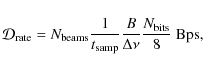
where
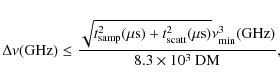
where
In practice, however, the scattering time can differ from this by a factor up to 100 (see Bhat et al. 2004). A smaller scattering time leads to the requirement of smaller - and thus more - frequency channels. To be on the safe side, we apply the highest frequency in the frequency band to Eq. (8) and divide the resulting scattering time by 100. Substituting
![\begin{figure}
\par\includegraphics[angle=-90,width=8.8cm]{eps/11939f09.eps}
\end{figure}](/articles/aa/full_html/2009/38/aa11939-09/img55.png) |
Figure 5:
Amount of data per second from a FAST pulsar survey as a
function of FoV. The calculation assumes a sampling time of
100 |
| Open with DEXTER | |
The number of operations required to search these data for normal
pulsars, millisecond pulsars and accelerated pulsars in binary systems
is approximately
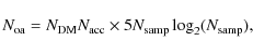 |
(9) |
where
4 Timing
In addition to being a very powerful search machine, FAST will also excel in the high-precision timing of pulsars. For a given pulsar, the timing precision roughly scales with the S/N of the observed pulse profile (Lorimer & Kramer 2005), and hence with telescope sensitivity. Until the Square Kilometre Array comes on-line (Sect. 5) FAST will have the largest sensitivity of all existing radio telescopes and will also be able to see a larger fraction of the sky than the Arecibo telescope. Consequently, FAST will be the telescope of choice for a number of high-precision timing experiments. While the Northern location of FAST means that it is unlikely to contribute significantly to the timing of, say, the Double Pulsar (PSR J0737-3039A/B, Burgay et al. 2003; Lyne et al. 2004), a major contribution of FAST will be the participation in the global Pulsar Timing Array efforts.
High-precision timing of a network of pulsars allows detection of a gravitational wave background by correlating the timing residuals of the pulsars (e.g. Jenet et al. 2006). Current efforts include PPTA (Parkes Pulsar Timing Array), EPTA (European Pulsar Timing Array) and NANOGrav (North American Nanohertz Observatory for Gravitational Waves). In terms of combination of sky coverage and sensitivity, FAST will only be matched by the European LEAP efforts (Large European Array for Pulsars), where the European 100-m class telescopes are combined to obtain Arecibo-like sensitivity for pulsar timing. This effort, however, has to overcome the challenge of coherently combining the signals between telescopes up to 2000 kilometres apart.
![\begin{figure}
\par\includegraphics[angle=-90,width=8.4cm]{eps/11939f10.eps}
\end{figure}](/articles/aa/full_html/2009/38/aa11939-09/img61.png) |
Figure 6:
Required computation power for real-time searching for
possibly accelerated fast and slow pulsars in the data from a FAST
pulsar survey as a function of FoV. The calculation assumes a
sampling time of 100 |
| Open with DEXTER | |
4.1 Pulsar timing array experiment
Following earlier work by Detweiler (1979) and Kaspi et al. (1994), pulsar
timing is now routinely used to constrain the amplitude of a
gravitational wave (GW) background. Currently the most stringent
limits have been placed by Jenet et al. (2006) from observations of seven
MSPs with the Parkes 64-m radio telescope (cf. Manchester 2008)
which constrain
![]() ,
the ratio of the energy density of
the GW background to the closure density to be
,
the ratio of the energy density of
the GW background to the closure density to be
![]() ,
where h is the dimensionless Hubble constant
defined as
,
where h is the dimensionless Hubble constant
defined as
![]() km s-1 Mpc-1. The
sensitivity that is needed to achieve a GW detection depends on
details of the Galaxy merger rate, since the GW background generated
by an ensemble of super-massive black holes distributed throughout the
Universe is expected to be the strongest signal to be detected. The
signal originating from such sources is expected at a level of
km s-1 Mpc-1. The
sensitivity that is needed to achieve a GW detection depends on
details of the Galaxy merger rate, since the GW background generated
by an ensemble of super-massive black holes distributed throughout the
Universe is expected to be the strongest signal to be detected. The
signal originating from such sources is expected at a level of
![]() (Enoki et al. 2004; Jaffe & Backer 2003; Wyithe & Loeb 2003). Simulations suggest that the timing of 20 pulsars with a
timing precision of 100 ns over five years would lead to a
sensitivity of
(Enoki et al. 2004; Jaffe & Backer 2003; Wyithe & Loeb 2003). Simulations suggest that the timing of 20 pulsars with a
timing precision of 100 ns over five years would lead to a
sensitivity of
![]() and hence to
a first direct detection of a GW background (Jenet et al. 2006). While
this is difficult with current technology, FAST will have the
sensitivity and sky coverage to make a major contribution to achieving
this goal.
and hence to
a first direct detection of a GW background (Jenet et al. 2006). While
this is difficult with current technology, FAST will have the
sensitivity and sky coverage to make a major contribution to achieving
this goal.
Here we estimate the amount of time needed to time the brightest MSPs, found by FAST, to high precision. For this simulation we choose model 2 from Table 2, which provides us with 670 MSPs. We take the 50 brightest of these and calculate the amount of time required for a S/N of 500, taking into account a conservative profile stabilisation time of five minutes. This leads to 24 h to time all 50 pulsars once. These numbers do not include accompanying low-frequency observations to allow correction for variations in interstellar dispersion. As expected, we found that the FoV provided by 19 beams had no impact on the timing performance, as there was no instance where two or more pulsars could be timed simultaneously.
5 FAST versus the SKA
The Square Kilometre Array (SKA) is a planned multi-purpose radio telescope with a collecting area approaching 1 million square metres. Although the exact design is not yet determined, it is likely to consist of aperture arrays to cover frequencies from 70 MHz up to 500 or even 800 MHz and 15-m dishes for the higher frequencies. About half of the elements will be placed within a 5-kilometre core of the SKA, the rest will be placed on spiral arms extending several thousands of kilometres outwards. Smits et al. (2009) have studied the performance of the SKA concerning pulsar surveys and timing. Here we will discuss the differences between these findings and those of the current paper.
A pulsar survey with FAST is straightforward compared to an SKA pulsar
survey. With the initial receiver, no beam-forming is required. The
future PAF does require beam-forming, but it does not need the vast
computational power of several peta-ops required for beam-forming the
SKA. Another benefit for FAST is that the data do not need to be
transported over long distances; the data processing can be performed
close to the dish. Also, the data rates and required computation power
for a real time acceleration search are much lower for the FAST
survey. This is mostly due to the smaller FoV of FAST, which is 10 to
50 times less than the FoV for an SKA pulsar survey, but also because
these data rates and computational power scale with the square of the
telescope diameter. The diameter of FAST is given by the illuminated
aperture of 300 m. For the SKA it is determined by the largest
baselines between the elements used in the survey. Smits et al. (2009)
estimate that the limits in computational power will restrict these
baselines to 1 kilometre. Because of this limitation, the telescope
sensitivity of a pulsar survey with the SKA is about
2000 m2K-1 which is equal to that of FAST. However, the
larger FoV of the SKA will not only enable a survey of a much larger
portion of the sky, but also allow for a longer dwell time per
pointing. The actual FoV of the SKA depends on the final design, but
at the very least it will be equal to the FoV of the 15-m dishes
which at 1.4 GHz is about 0.64 deg2. For comparison, a
reasonable assumption would be that an SKA survey has a dwell time of
40 min versus 10 min for a FAST survey. This makes the survey
sensitivity of the SKA twice that of FAST. Compared to the initial
19-beam receiver of FAST, a pulsar survey with the SKA would be about
2.5 times faster, but with the 100-beam PAF, the survey speed of FAST
would be twice that of the SKA. Moreover, because the elements of the
SKA are fully steerable, the SKA will be able to survey a much larger
part of the sky and with its latitude of about -30![]() this
includes almost the entire Galactic plane.
this
includes almost the entire Galactic plane.
Timing pulsars with the SKA can be performed with a considerable fraction of the full collecting area, providing a sensitivity close to 10 000 m2 K-1. Also, the large FoV of the SKA allows timing of many pulsars simultaneously (but depending on the SKA design, this might not be the case when using the SKA for a pulsar timing array). Even the future 100-beam PAF of FAST only has a quarter of the FoV of 15-m dishes and should the SKA be equipped with PAFs or mid-frequency aperture arrays, its FoV increases significantly to 20 deg2 or even 250 deg2.
Given that FAST will be operational well ahead of the full SKA, it is likely to be the most powerful telescope to perform pulsar science in the next decade and will remain an outstanding instrument for pulsar science, complementing the SKA once it is operational.
6 Summary
The FAST pulsar survey simulation in Sect. 2 shows that, despite the small natural beam-size and limitations in zenith angle, FAST will be a formidable instrument for finding pulsars.
A tradeoff between the number of pulsars and total observation time
can be determined from Table 2. With the initial 19-beam
receiver about 5200 previously unknown pulsars, including 460 MSPs, can be found in a survey of about 230 days of the visible
part of the Galactic plane with
![]() .
With a 100-beam
receiver 5900 previously unknown pulsars can be found in
the same region in 130 days, including about 540 previously unknown MSPs. The 100-beam receiver will also enable an
all-sky survey yielding 4300 previously unknown pulsars
in 300 days. Further, we estimate that a 470-h survey of M 31 and
M 33 would yield between 50 and 100 extra-Galactic pulsars.
.
With a 100-beam
receiver 5900 previously unknown pulsars can be found in
the same region in 130 days, including about 540 previously unknown MSPs. The 100-beam receiver will also enable an
all-sky survey yielding 4300 previously unknown pulsars
in 300 days. Further, we estimate that a 470-h survey of M 31 and
M 33 would yield between 50 and 100 extra-Galactic pulsars.
A pulsar survey with the 19-beam receiver will produce just under 500 MB of data per second. Depending on the survey, this leads to a total of 17 or 33 peta-bytes. The major part of a real-time acceleration search of these data would require 9 tera-ops. After 2014, such data rates and processing power should be very feasible.
FAST will also be able to contribute to the existing efforts to detect a gravitational wave background by timing a large number of MSPs to high precision. Although the visible sky of FAST is limited to 58% of the entire sky, those pulsars that are visible to FAST can be timed to great precision very quickly. A simulation in Sect. 4 suggests that the 50 brightest MSPs, visible to FAST can be timed to a S/N of 500 in just 24 h.
Compared to a pulsar survey with the SKA, FAST will match the sensitivity of the SKA, but the large FoV of the SKA will allow for longer dwell times and make the survey faster, at least for the initial 19-beam configuration of FAST. Also, the SKA will be able to survey a much larger part of the sky. However, having a single dish rather than many elements spread over a large area significantly reduces the required data rates and computational power. When timing pulsars for a pulsar timing array, the SKA will have much more sensitivity than FAST, since the SKA can use almost the full collecting area in this case. Also, the larger FoV of the SKA will allow timing of many pulsars simultaneously, although this will probably not benefit the timing of the limited number of pulsars from the timing array. Given that FAST will be operational well ahead of the full SKA, it will provide the best prospects for pulsar science in the next decade.
Acknowledgements
We would like to thank the referee, Scott Ransom, for his useful suggestions and comments. The authors have made use of the ATNF Pulsar Catalogue which can be found at http://www.atnf.csiro.au/research/pulsar/psrcat. This effort/activity is supported by the European Community Framework Programme 6, Square Kilometre Array Design Studies (SKADS), contract No. 011938. D.R.L. is supported by a Research Challenge Grant from West Virginia EPSCoR.
References
- Berkhuijsen, E. M. 1984, A&A, 140, 431 [NASA ADS]
- Bhat, N. D. R., Cordes, J. M., Camilo, F., Nice, D. J., & Lorimer, D. R. 2004, ApJ, 605, 759 [NASA ADS] [CrossRef] (In the text)
- Bonanos, A. Z., Stanek, K. Z., Kudritzki, R. P., et al. 2006, ApJ, 652, 313 [NASA ADS] [CrossRef]
- Burgay, M., D'Amico, N., Possenti, A., et al. 2003, Nature, 426, 531 [NASA ADS] [CrossRef]
- Burgay, M., Joshi, B. C., D'Amico, N., et al. 2006, MNRAS, 368, 283 [NASA ADS] (In the text)
- Corbelli, E., & Salucci, P. 2000, MNRAS, 311, 441 [NASA ADS] [CrossRef]
- Cordes, J. M., & Chernoff, D. F. 1997, ApJ, 482, 971 [NASA ADS] [CrossRef] (In the text)
- Cordes, J. M., & Lazio, T. J. W. 2002, ArXiv Astrophysics e-prints (In the text)
- Detweiler, S. 1979, ApJ, 234, 1100 [NASA ADS] [CrossRef] (In the text)
- Edwards, R. T., Bailes, M., van Straten, W., & Britton, M. C. 2001, MNRAS, 326, 358 [NASA ADS] [CrossRef]
- Enoki, M., Inoue, K. T., Nagashima, M., & Sugiyama, N. 2004, ApJ, 615, 19 [NASA ADS] [CrossRef]
- Faucher-Giguère, C.-A., & Kaspi, V. M. 2006, ApJ, 643, 332 [NASA ADS] [CrossRef] (In the text)
- Gordon, S. M., Kirshner, R. P., Long, K. S., et al. 1998, ApJS, 117, 89 [NASA ADS] [CrossRef]
- Jacoby, B. A., Bailes, M., Ord, S. M., Knight, H. S., & Hotan, A. W. 2007, ApJ, 656, 408 [NASA ADS] [CrossRef]
- Jaffe, A. H., & Backer, D. C. 2003, ApJ, 583, 616 [NASA ADS] [CrossRef]
- Jenet, F. A., Hobbs, G. B., Lee, K. J., & Manchester, R. N. 2005, ApJ, 625, L123 [NASA ADS] [CrossRef] (In the text)
- Jenet, F. A., Hobbs, G. B., van Straten, W., et al. 2006, ApJ, 653, 1571 [NASA ADS] [CrossRef] (In the text)
- Jin, C. J., Nan, R. D., & Gan, H. Q. 2008, in IAU Symp., 248, 178 (In the text)
- Kaspi, V. M., Taylor, J. H., & Ryba, M. F. 1994, ApJ, 428, 713 [NASA ADS] [CrossRef] (In the text)
- Lorimer, D. R., & Kramer, M. 2005, Handbook of Pulsar Astronomy (Cambridge University Press) (In the text)
- Lorimer, D. R., Yates, J. A., Lyne, A. G., & Gould, D. M. 1995, MNRAS, 273, 411 [NASA ADS] (In the text)
- Lorimer, D. R., Faulkner, A. J., Lyne, A. G., et al. 2006, MNRAS, 372, 777 [NASA ADS] [CrossRef] (In the text)
- Lyne, A. G., Burgay, M., Kramer, M., et al. 2004, Science, 303, 1153 [NASA ADS] [CrossRef]
- Lyne, A. G., Manchester, R. N., Lorimer, D. R., et al. 1998, MNRAS, 295, 743 [NASA ADS] [CrossRef]
- Manchester, R. N. 2008, in 40 Years of Pulsars: Millisecond Pulsars, Magnetars and More, ed. C. Bassa, Z. Wang, A. Cumming, & V. M. Kaspi, AIP Conf. Ser., 983, 584 (In the text)
- Manchester, R. N., Lyne, A. G., D'Amico, N., et al. 1996, MNRAS, 279, 1235 [NASA ADS]
- Manchester, R. N., Lyne, A. G., Camilo, F., et al. 2001, MNRAS, 328, 17 [NASA ADS] [CrossRef]
- Manchester, R. N., Hobbs, G. B., Teoh, A., & Hobbs, M. 2005, AJ, 129, 1993 [NASA ADS] [CrossRef]
- Nan, R. 2006, Science in China Series G: Physics, Mechanics and Astronomy, 49, 2, 129
- Nan, R. 2008, in SPIE Conf. Ser., 7012
- Nan, R.-D., Wang, Q.-M., Zhu, L.-C., et al. 2006, Chinese J. Astron. Astrophys. Suppl., 6, 020000 (In the text)
- Ribas, I., Jordi, C., Vilardell, F., et al. 2005, ApJ, 635, L37 [NASA ADS] [CrossRef]
- Seigar, M. S., Barth, A. J., & Bullock, J. S. 2008, MNRAS, 389, 1911 [NASA ADS] [CrossRef]
- Smits, R., Kramer, M., Stappers, B., et al. 2009, A&A, 493, 1161 [NASA ADS] [CrossRef] [EDP Sciences] (In the text)
- Wyithe, J. S. B., & Loeb, A. 2003, ApJ, 590, 691 [NASA ADS] [CrossRef]
Footnotes
All Tables
Table 1: Expected system parameters of FAST and the pulsar survey.
Table 2: Total survey time for different FAST surveys.
Table 3: Parameters of M 31 and M 33.
Table 4:
Total amount of data from different survey models (see
Table 2). Except for model 7, the surveys are limited
in Galactic longitude by
![]() .
.
All Figures
| |
Figure 1:
Number of normal pulsars and MSPs detected in
simulations of FAST surveys of the Galactic plane as a function of
observation frequency. The surveys were limited in Galactic
longitude by
|
| Open with DEXTER | |
| In the text | |
| |
Figure 2:
Number of normal pulsars and MSPs detected in
simulations of FAST surveys as a function of observation time per
pointing. The surveys were limited in Galactic latitude and
longitude by
|
| Open with DEXTER | |
| In the text | |
| |
Figure 3:
Distribution of detected normal pulsars and MSPs for
different models. The top left plot shows the distribution of
normal pulsars from models 1 (similar to model 3) and 5.
The top right plot shows the distribution of normal pulsars from models 2
(similar to model 4) and 6. The two plots in the middle show
the distribution of millisecond pulsars from the same models as
the plot directly above. The bottom plot shows a Hammer-Aitoff
projection of the distribution of normal pulsars and millisecond
pulsars from model 7 in galactic coordinates. The black and white
striped boxes mark the areas defined by
|
| Open with DEXTER | |
| In the text | |
| |
Figure 4:
Total amount of data from a FAST pulsar survey as a function
of the total survey field. The calculation assumes a bandwidth of
400 MHz, a FoV
|
| Open with DEXTER | |
| In the text | |
| |
Figure 5:
Amount of data per second from a FAST pulsar survey as a
function of FoV. The calculation assumes a sampling time of
100 |
| Open with DEXTER | |
| In the text | |
| |
Figure 6:
Required computation power for real-time searching for
possibly accelerated fast and slow pulsars in the data from a FAST
pulsar survey as a function of FoV. The calculation assumes a
sampling time of 100 |
| Open with DEXTER | |
| In the text | |
Copyright ESO 2009
Current usage metrics show cumulative count of Article Views (full-text article views including HTML views, PDF and ePub downloads, according to the available data) and Abstracts Views on Vision4Press platform.
Data correspond to usage on the plateform after 2015. The current usage metrics is available 48-96 hours after online publication and is updated daily on week days.
Initial download of the metrics may take a while.